A novel method for the in situ calibration of flow effects on a phosphate passive sampler

Abstract

Monitoring of nutrients including phosphate in the aquatic environment remains a challenge. In the last decade passive sampling techniques have been developed that facilitates the time integrated monitoring of phosphate (P) through the use of an iron hydroxide (ferrihydrite) to sequester dissolved phosphate from solution. These methods rely on established techniques to negate the effects of flow (and associated turbulence) and control the rate at which chemicals accumulate within passive samplers. In this study we present a phosphate sampler within which a suspension of ferrihydrite is contained behind a commercially available membrane. Accumulation of dissolved phosphates into the P-sampler is governed by the rate at which ions are diffusing through the membrane and the water boundary layer (WBL). As the WBL changes subject to flow we have adopted an in situ calibration technique based on the dissolution of gypsum to predict the change in the rate of uptake dependent on flow. Here we demonstrate that the loss of gypsum from the passive flow monitor (PFM) can be used to predict the sampling rate (the volume of water extracted per day) for phosphate as a function of water velocity. The outcome of this study presents a new in-field tool for more accurate prediction of the effect of flow/turbulence on the uptake kinetics into passive samplers that is controlled by the diffusion of the chemical of interest through the stagnant water boundary layer.

---

Introduction

Macronutrients such as nitrogen and phosphorous have been limiting components governing primary production in many surface waters. Consequently, the input of nutrients in excess of a systems requirement can have many effects that impact upon the ecology of water bodies and the aesthetic or human specific use of the water body. For example, eutrophication can promote the proliferation of fast growing primary producers that cause a decrease in water clarity and quality, affecting the commercial or recreational application to which the water can be applied. Should the eutrophic status of the system persist, changes in the ecological diversity may occur (Cloern,¹ Hartog,² Lavery et al.,³ Sanders and Baron-Szabo,⁴ Tett et al.,⁵ Maritorena et al.,⁶ Thomsen and McGlathery⁷). This risk to ecosystem health has lead to the introduction of ongoing monitoring programs to assess the trophic status of aquatic environments impacted upon by human activities. Such programs can use automated collection or analysis equipment, however, the cost to purchase and maintain these automated devices often makes it impractical to implement their use at multiple sites. Furthermore the monitoring of nutrients (nitrogen and phosphorus) predominantly involves the manual collection of grab water samples at regular time intervals for laboratory analysis.

Methods have been developed and applied that utilise ferrihydrite, an iron(oxy)hydroxide adsorbent, for the extraction of filterable reactive phosphate (FRP) (Zhang et al.,⁸ Müller et al.,⁹ Chardon et al.,¹⁰ Baldwin et al.,¹¹ Dils and Heathwaite¹² Müller et al.,¹³ Shao et al.,¹⁴ Van Rimesdijk et al.,¹⁵ Willett et al.¹⁶). Reactive phosphorus has been extracted from soil and water samples through the use of iron impregnated filter paper (Chardon et al.,¹⁰ Baldwin et al.,¹¹ Dils and Heathwaite¹²) and iron oxide filled dialysis bags (Freese et al.¹⁷). From these methods quantitative passive sampling techniques have been developed exploiting ferrihydrite as a sink for filterable reactive phosphorus inside a diffusion gradient thin-film (DGT) contained within a gel matrix (Zhang et al.⁸) or inside the P-trap where the ferrihydrite is suspended in an aqueous solution contained behind a semipermeable membrane (Müller et al.⁹).

Fick's first law has been adapted to model the uptake of an analyte into a passive sampling device, so that the change in concentration [ΔC = external water concentration (Cw) − water concentration within the sampling device (Cs)] across a diffusion barrier is given by:

ΔC = F δ/D (1)

where F is the flux of the diffusing molecules, δ is the thickness of the diffusion membrane and D is the diffusion coefficient of the chemical of interest in water.

Within passive sampler devices the analyte of interest is removed from solution through the use of a selective receiving phase. As a result the concentration of analyte that is unbound by the sampling phase and free in solution within the sampling device (Cs) is effectively zero. Thus Equation 1 can be simplified to:

Cw = F δ/D (2)

By incorporating the definition of flux, F = M/At [where M is the mass of analyte diffused through a known area (A) over a given time (t)], Equation 2 can be expressed as

Cw = M δ/DAt (3)

For samplers to provide time-integrated environmental concentrations a fundamental requirement is that they operate in the linear kinetic phase of uptake where Cw≫C_s/compound specific partitioning coefficient or K_sw and the co-diffusion of chemicals from the sampler to the environment can be neglected (see reviews for further details Vrana et al.,¹⁸ Seethapathy et al.,¹⁹ Ouyang and Pawliszyn,²⁰ Stuer-Lauridsen²¹). When it is known that the sampler is operating in the linear phase of uptake, Equation 3 can be further simplified to

Cw = M_s/Rs t (4)

Where M_s is the mass of chemical determined in a given sampler, t is the period that the sampler has been deployed and Rs is a chemical specific sampling rate equal to DA/δ. The sampling rate can be determined in calibration experiments when Cw, M_s and t are known, and is a measure of the volume of water that is cleared by the sampler per unit time (L/day).

The sampling rate into passive samplers (Rs) is controlled by the diffusion of the solute through the water boundary layer (WBL) and/or across the partitioning membrane (Huckins et al.²²) or an artificial diffusion barrier such as the diffusion gel within the DGT (Zhang and Davison²³). For samplers where the WBL governs the Rs, the Rs will change depending on environmental conditions and in particular the water velocity at the surface of the sampler (Stephens et al.,²⁴ Vrana et al.,²⁵ Huckins et al.²⁶). In partition based samplers that can be modelled by the chemical specific Ksw, the introduction of performance reference chemicals (PRCs) has enabled the in-situ calibration of the effect of environmental factors on chemical specific sampling rates (Huckins et al.²²). The introduction of PRCs has thus become an important quality control/quality assurance (QCQA) technique that allows in-field calibration of Rs. The use of PRCs is not compatible with samplers where the chemical of interest is captured through chemical modification such as with the adsorbent ferrihydrite, where it is proposed that complexes of non-protonated bidentate binuclear species Fe2PO4 form at the iron water interface (Arai and Sparks²⁷), because the loss of any pre loaded chemicals from the sampler is not isotropic (Greenwood et al.²⁸). In addition, the use of PRCs does not adequately model the uptake of compounds with low membrane-water partioning coefficients as the Rs is determined by the thickness of the partitioning membrane and not by change in the WBL (Huckins et al.²²). However as many passive samplers do not employ an artificial diffusion boundary layer and the uptake may be subject to change in the thickness of the WBL, a method is desired that can be used to model the site specific changes in the Rs for analytes accumulated within adsorbent passive samplers.

Plaster dissolution has been used successfully to assess water movement (flow and turbulence) in field experiments and, as early as 1968, Muus introduced the method to measure turbulent water motion in relation to the growth and distribution of benthic aquatic organisms by monitoring the mass lost from plaster spheres (Muus²⁹). This method was expanded upon to investigate the effects of flow on the mechanisms governing the rate of nutrient uptake into algae and plants through the use of plaster “clod-cards” to measure both the relative water velocity and the degree to which diffusion across a boundary layer is influenced by water motion (Doty³⁰). Studies undertaken correlating water flow across plaster devices with the mass lost over time have investigated the effect of flow conditions, velocity, temperature and salinity on the rate of dissolution (Hart et al.,³¹ Howerton and Boyd,³² Jokiel and Morrissey,³³ Komatsu and Kawai,³⁴ Petticrew and Kalff,³⁵Porteret al.³⁶). These studies have shown that for a given salinity and temperature the loss of a specific plaster material, such as calcium sulfate, over a given surface area can be described from an empirical calibration exponent that relates the loss of plaster (k_PFM in g/day) to the velocity and/or turbulence of the water. However, while the use of plaster devices has been applied to the determination of mass-transfer rates for the uptake of dissolved material by aquatic organisms (Doty,³⁰ Jokiel and Morrissey³³) it has not been applied to describe uptake into passive samplers.

As there has been limited application of ferrihydrite as a sampling phase within quantitative passive samplers where the WBL thickness is controlling Rs, the aim of this study was to assess the role of flow/turbulence on the uptake of phosphate into the phosphate sampler (P-sampler). Furthermore, in this study we evaluate a cost effective and rapid external calibration technique for in-field adjustment of laboratory derived calibration data. To achieve this aim, the sampling rate of the P-sampler and the rate of plaster lost per day from co-deployed PFMs (k_PFM) were calibrated over time when exposed to various water velocities.

Materials and methods

Reagents

Analytical reagent iron(III) nitrate nonahydrate (Fe(NO₃)₃·9H₂O), potassium dihydrogen phosphate (KH₂PO₄), and ammonium molybdate tetrahydrate ((NH₄)₆Mo₇O₂₄·4H₂O) were obtained from Sigma-Aldrich (Australia). Sulfuric acid and potassium antimony tartrate (APT/KSbOC₄H₄O₆) were obtained from BDH Chemicals (Biolab, Australia). Sodium hydroxide was obtained from Lab-scan Ltd (Poland). Hydrochloric acid was obtained from Univar Ajax Finechem (Australia). Any glassware, tools or equipment that were in contact with either the sampling phase or the extracting reagents were cleaned using acetone (Merck Australia) and washed with dilute acid (3% HCl) before a final rinse with ultra pure MilliQ H₂O prior to use.

Plaster flow monitors (PFM)

The design of the plaster flow monitoring devices was such that the surface of the exposed plaster was equal to that of the P-sampler with an area of 13.85 cm². The PFM devices are prepared from Dental Plaster (BORAL) cast into 120 mL specimen containers [internal dimensions: 42 mm Ø, 105 mm high] (SARSTEDT) that were altered with the addition of a cable tie (Weller) secured in place with a construction adhesive (Selleys clear liquid nails) to allow for the PFM to be attached to a mooring when deployed in the field (Fig. 1). The altered containers were then filled with a 1:2 plaster mix prepared using 80 mL deionised water and 160 g plaster powder. Once firm (∼5 minutes after the plaster is first mixed with water), the containers were capped to prevent drying and stored at 4 °C.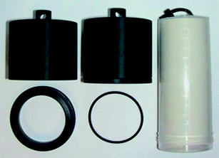

Fig. 1 A view of a P-sampler (centre top) and PFM (right) prepared for deployment. Also shown are the disassembled parts of the P-sampler chamber including the chamber body (top left), the screw cap (bottom left) and rubber o-ring (bottom centre).

Phosphate samplers

The design of the chamber of the P-sampler was governed by the size of the commercially available membranes used as a diffusion barrier between the 50 mL sampling phase and the sampled waters. The cylindrical chamber [dimensions: external – 55 mm diameter, 49 mm high; internal (behind membrane) – 42 mm diameter, 29 mm high] holds approximately 40 mL of solution (see Fig. 1). The membrane used is similar (in size and material) to those used in the construction of the polar organic chemical integrated samplers developed at the USGS (Alvarez et al.³⁷) and the Chemcatcher sampler developed at the University of Portsmouth (Kingston et al.³⁸); thus the surface area through which molecules are diffusing into the three different devices is comparable. When assembled, the membrane has an exposed surface area of 13.85 cm² (diameter of 42 mm) after being secured in place using an acetyl o-ring (A and B seals, MN7-043-2/ORM043.00 002.00 047.00). The chambers were custom ordered for the development of the P-samplers.

The Z-bind 200 membrane [47 mm diameter (0.2 nm pore)] (PALL life sciences) used in the P-samplers as a diffusion barrier consists of a modified polyethersulfone. This membrane was selected because the low-protein binding properties exhibited by the polyethersulfone allow for long deployment periods to be undertaken with less risk of biological fouling (Schäfer et al.,³⁹ Kochkodan et al.,⁴⁰ Wang et al.,⁴¹ Knoell et al.,⁴² Pieracci et al.,⁴³ Flemming and Schaule⁴⁴) or degradation (Gorecki and Namiesnik,⁴⁵ Schäfer et al.⁴⁶). The membranes were conditioned and purified by submerging in methanol (20 mL per membrane) for 20 minutes followed by a 5 minute immersion in MilliQ H₂O. The conditioned membranes were stored in MilliQ H₂O at 4 °C for up to two weeks prior to use.

The suspension of ferrihydrite used as a sampling phase for the accumulation of phosphate was prepared through the slow addition of 600 mL 1 M NaOH to 1 L of 0.2 M iron(III) nitrate nonahydrate to establish a pH of approximately 7. The supernatant was decanted and the precipitated ferrihydrite washed 3 times with MilliQ H₂O. The final volume of the ferrihydrite suspension, containing approximately 29.15 g of iron(oxy)hydroxide, was adjusted to 1 L and stored in the dark at 4 °C for up to a month prior to use. The pH of the ferrihydrite stock was checked prior to addition to the sampling chambers to ensure that a neutral pH is maintained. Titration experiments on the ferrihydrite were undertaken to determine a maximum adsorption capacity of 9.76 × 10⁻⁴ mol P/g.

P-samplers were prepared with the addition of a 20 mL aliquot of the ferrihydrite suspension added to each sampling chamber and the chamber filled with MilliQ H₂O such that each P-sampler contained 0.322 g of iron(III). The membrane was placed on the surface of the solution extending across the o-ring. The membrane seals the sampler when the cap is tightened. Samplers were deployed with the membrane facing down to allow for the ferrihydrite particles to settle over the membrane. To prevent any air bubbles forming between the water and the membrane, samplers were submerged facing upwards and then turned downwards underwater.

Upon retrieval of the P-samplers the ferrihydrite was removed from solution viacentrifugation and dissolved in 50 mL of 0.25 M H₂SO₄ over 16 hours. Analysis of the FRP concentrations within the P-sampler extract was undertaken using the molybdenum blue method. As iron is known to produce a false positive reading during the molybdenum blue test at concentrations of > 0.02 g Fe/L, all P-sampler extracts were diluted (1/20) prior to undertaking analysis (Fogg and Wilkinson,⁴⁷ Kowalenko and Babuin⁴⁸).

The analytical reaction was undertaken in an acetone/acid/MilliQ washed 25 mL volumetric flask to which a 1 mL aliquot of dilute P-sampler extract was added to a 25 mL reaction solution containing a final concentration of 0.21 mM H₂SO₄, 0.77 µM (NH₄)₆Mo₇O₂₄·4H₂O, 0.066 µM APT/KSbOC₄H₄O₆ and 0.47 µM ascorbic acid. The reaction mix was stirred and the absorbance determined at 882 nm after five minutes using a UV spectrophotometer (Hitachi, Japan). As the reaction product is time sensitive, all absorbance readings were taken within 5–10 minutes of the sample addition to the reaction mixture. This prevented readings being obtained while the reaction is still occurring (<5 minutes of reaction time) or after the reaction product has begun to degrade (>10 minutes of reaction time) (Murphy and Riley,⁴⁹ Pai et al.⁵⁰). Standards of 0, 0.05, 0.12, 0.24 and 0.48 mg P/L were used to establish a calibration curve and extracts obtained from blank P-samplers were included during the analysis of all samples obtained for each experiment undertaken.

Experimental chamber

Calibration experiments for both the PFM loss and the uptake of phosphate in the sampler were undertaken in an insulated, 1400 L stainless steel calibration tank. A custom built stainless steel turntable was installed within the tank to which the passive samplers can be attached. A 12 V DC drive motor (Hitachi, Japan) controlled the movement of the turntable from which the P-sampler and PFM devices were deployed from arms that extended 32 cm from the rotor. The rotation of the turntable can be set to between 2.5 and 50 revolutions per minute, the movement of which corresponds to a laminar flow rate of 4.18–83.8 cm/s at a distance of 32 cm from the rotor. Prior to the undertaking of this experiment the tank was cleaned using acetone and rinsed with a wash of dilute acid (3% HCl) and flushed with mains water. The tank was filled with 1400 L of mains water for the undertaking of the experiments.

The tank was kept closed throughout the experiments to prevent atmospheric deposition into the system. This also prevents algal growth (which could affect the availability of phosphate) and reduces variations in temperature, which was not controlled in the experiments, but which is typically relatively stable due to the position of the tank in a protected site, the insulation of the tank and the large water volume in the tank. A Thermochron iButton (Maxim Integrated Products, USA), part number DS1921L-F50) was submerged within an air tight container attached to the turntable of the tank to record the water temperature hourly over the experimental period.

Two methods were used to assess the velocity of the water within the tank and at the sampler surface. The first involved the use of a Flowwatch – Air or Liquid Flow Measurement Instrument (ALFMI) from JDC Electronic SA (Australia). The Flowwatch ALFMI allows measurements of water velocity greater than 0.1 m/s. As the design of the tank is not conducive to the production of laminar flow across the diffusive surface of the samplers, the water velocity was measured using the Flowwatch ALFMI, at a distance of ∼32 cm from the rotor. The water velocity relative to the samplers as they are moved through the water was determined by substraction of the water velocity measured using the Flowwatch ALFMI from the rotational speed. The results obtained are shown in Table 1. The use of a passive flow monitor (PFM) as the second flow monitoring method has been introduced to investigate the application of these devices in the assessment of flow effects at the diffusive surface of a passive sampling device.

Table 1 Water velocity and temperature within the experimental tank and the corresponding rate of mass loss from PFM devices

	Velocity [cm/s]			Temperature [°C]	kPFM			kPFM
	Turntable^a	Water ^b	Adjacent to sampler	Average (min/max)	[g/day]	SD	r^2	[g/day/cm^2]	SD	r^2
a Nominal rotation speed. b Manual measurement using the Flowwatch ALFMI device.
Still water	0	0	0	16.2 (16.0–16.5)	0.56	0.01	0.98	0.04	0.001	0.98
1.5 rpm	5.7	2.4	3.4	16.5 (16.0–19.5)	0.57	0.02	0.94	0.04	0.002	0.94
3 rpm	10.3	4.3	6.0	18.5 (17.0–19.0)	1.43	0.02	0.99	0.10	0.001	0.99
8 rpm	27.4	11.3	16.1	19.3 (18.0–20.5)	2.74	0.03	0.99	0.20	0.002	0.99
12 rpm	41.1	17	24.1	22.0 (21.0–22.5)	3.99	0.03	0.99	0.29	0.002	0.99

---

Experimental conditions

PFM and P-samplers were co-deployed in the experimental chamber containing 1400 L of mains water spiked with 2.4 mg P/L. Five experiments, each consisting of a ten day sampler deployment period were carried out. During these deployments, samplers were exposed in replicates to either negligible flow or stimulated flow conditions, which equated to flow rates of 0, 3.4, 6.0, 16, 24 cm/s (Table 1).

The mass of the individual PFMs was recorded prior to deployment and up to twice daily over the deployment period through the use of a mobile balance (Quad Beam 311g) after excess water was removed with a cellulose based tissue (Kimwipes, Kimberly-Clark). A new set of three PFMs were introduced to the tank at the beginning of each consecutive deployment period. Twelve P-samplers were prepared per deployment; 10 of which were deployed in the tank and retrieved in duplicate after 1, 3, 5, 7 and 10 days of exposure. The remaining two P-samplers were analysed as blanks to establish the FRP concentration within the samplers at the time of deployment.

Grab water samples (30 mL unfiltered and 15 mL filtered) were obtained at each time point at which samplers were deployed and retrieved from the tank. Terumo eccentric tip syringes were used to collect the water samples and particulate matter was removed from the sample using a syringe filter (MiniStart Highflow, Vivascience). All water samples were stored at 4 °C (for up to 48 hours) or −21 °C (for up to 2 months) in Falcon tubes (BD Australia/New Zealand) of 15 and 50 mL capacity, prior to FRP analysis using the molybdenum blue method.

Results and discussion

Calibration of plaster loss at different water velocities

The mass of the PFM devices determined daily when deployed in triplicate under negligible flow and at 4 different rotational speeds showed that the loss of mass was consistently linear over the deployment periods (r² > 0.95 see Table 1). The mass lost from the deployed PFM (PFM_L) ranged from 4.95–40.1 g or 0.46–3.9 g/day (0.04–0.29 g/day/cm² projected surface area) dependent on the flow rates to which the devices were exposed (Fig. 2). It should be noted that under still and very low flow conditions there was little difference in the mass lost from the PFM. Hence it appears that at near stagnant conditions the PFM can not provide an accurate prediction for the effect of flow on Rs (i.e. below a threshold flow of 3.35 cm/s). Thus the PFM data obtained in the absence of flow was excluded from analysis when a significant linear relationship (r² = 0.98) was found between the loss of mass from the PFM and the rotation/nominal water velocity (Fig. 3).Using the observed k_PFM the calculated water velocities (cm/s) can be described by:

v (cm/s) = (k_PFM − 0.26)/0.15 (5)

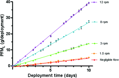Fig. 2 Mass lost from the deployed PFM when exposed to different water velocities (cm/s).

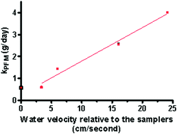Fig. 3 Mass per day lost from the PFM devices when exposed to different water velocities. (k_PFM at 0 cm/s excluded from regression).

Following the preparation of the plaster casts all PFMs were kept moist to prevent drying and maintain a constant mass, but were not saturated with water prior to deployment to avoid the dissolution of calcium sulfate during storage prior to deployment. However, there was a recorded increase in the mass of all devices over the first 24 h of deployment when either stationary or moved through the water at 1.5 rpm. The increase in mass can be attributed to the plaster becoming saturated with water following submersion in the tank; the extrapolation of the value of X when Y = 0 from the plot of mass lost (Fig. 2) can be used to determine the time needed for each PFM set to become saturated under the 5 different flow conditions.

A delay of 40.9, 37.6, 6.7, 4.9 and 3.8 hours was established as the time taken for a uniform decrease in the initial PFM mass to occur when exposed to no flow or the flow produced at 1.5, 3, 8 and 12 rpm respectively. An exponential relationship between PFM_L and the time (days) lapse before an overall loss in mass occurs is illustrated in Fig. 4. The exponential slope is modelled by Equation 6 and can be used to take the “re-hydration” into account when determining k_PFM by subtracting the delay from the total deployment period.

Re-hydration correction [Days] = 7.43 exp (−0.32 PFM_L) + 0.18 (6)

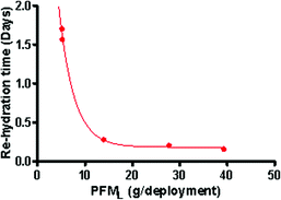Fig. 4 Lag prior to linear rate for each k_PFM recorded.

Time and flow dependent uptake of FRP by the P-samplers

The reproducibility of results was determined using mean normalised differences for the 2 PFM replicates obtained at each time point. The %-normalised difference (ND) was calculated by dividing the difference between the two values by their average. The mean normalised difference was calculated to be 10, 9.6, 3.5, 16 and 8.7% for the replicates deployed at 0.0, 1.5, 3.0, 8.0 and 12 rpm respectively. The uptake of phosphate into the samplers (Fig. 5) described using linear regressions ranged from about 3.5 to 33 µg P/L depending on water velocity. It is interesting to note that while there is a high scatter in the linear uptake of P into the P-samplers when moved at 3 rpm (r² = 0.85) this data set has the highest reproducibility between replicates. The average uptake of FRP (g/day) as shown by the slope of the linear regressions in Fig. 5 was used in the calculation of the Rs dependent on water velocity (Table 2). The linear increase in P within the samplers demonstrates that equilibrium had not been established between the concentration of FRP in the water reservoir and in the ferrihydrite sampling phase. Assuming that linear uptake was occurring (Ouyang and Pawliszyn⁵¹); the sampling rate (Rs) was determined using Equation 4 to range between 6.5 mL per day to approx. 60 mL per day dependent on flow (Table 2).

Table 2 P-sampler sampling rates (Rs) determined from the average FRP concentration in the water (Cw) and accumulated by the P-samplers (Cs) when deployed at different water velocities

Calculated water velocity relative to the sampling devices (cm/s)	FRP concentration [µg as P/L]				Increase in FRP within P-samplers			Sampling Rate [L/day]
	Cw	SD	Cs	SD	ug/day	SD	r^2	Rs	SD
Negligible flow	2.85	0.19	3.69	0.24	0.012	0.001	0.715	0.007	0.001
3.35	2.59	0.19	11.93	1.66	0.065	0.003	0.921	0.023	0.003
6.02	2.54	0.12	18.12	3.13	0.091	0.006	0.855	0.036	0.006
16.06	2.76	0.24	30.04	1.05	0.156	0.005	0.954	0.055	0.002
24.09	2.66	0.07	31.95	1.58	0.143	0.007	0.922	0.060	0.003

---

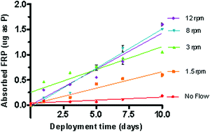Fig. 5 Change in the mass of P adsorbed by the phosphate samplers over time when exposed to different flow velocities.

A plot of the calculated Rs as a function of flow or k_PFM (Fig. 6) demonstrated that there is a non-linear relationship between the Rs and the measure of flow velocity, whether direct or through the use of the PFM. The application of a logarithmic trend line to the data plotted in Fig. 6 reveals that the sampling rate can be predicted (r² = 0.99) using:

Rs = 0.006 + 0.011(v)^0.52 (7)

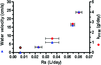Fig. 6 Sampling rate (Rs) for FRP uptake into the P-samplers dependent on water velocity and the corresponding k_PFM.

Hence this suggests an increase in Rs of √2 as the water velocity doubles. This relationship is similar to that produced by a model developed for the calculation of the diffusion boundary layer thickness adjacent to a flat plate (Schlichting 1968 as cited by Nobel⁵²) or leaf (Nobel⁵²), and indicates that the thickness of the water side diffusion boundary layer is controlling the sampling rate of the P-sampler. The fact that the sampling rate changes as a function of water velocity implies that potential errors may be introduced when estimating the mean water concentration of a chemical. In principle one can expect accurate predictions when the concentration is independent from flow. However if flow correlates with the concentration we can expect an over prediction of Cw since the sampler extracts a large volume of water at high flow when the concentration is high. In reverse if the concentration is inversely related to flow than we can expect an under prediction (i.e. low Rs at high Cw). A relationship between flow and concentration is not typical except during floods when either of the above scenarios may occur (i.e. high runoff of chemicals or dilution in environmental waters) and thus introduce a dependence between flow and concentration.

The use of the P-sampler as a time integrated assessment tool can only occur when the rate of FRP uptake can be successfully corrected for the effects of flow. The use of the PFM device to assess the effects of flow acting upon the P-sampler facilitates the correction of Rs for flow such that Rs can be calculated using a combination of Equation 7 and Equation 5 to produce

Rs = 0.006 + 0.011 [(k_PFM − 0.26)/0.15]^0.52 (8)

The incorporation of Equation 8 into Equation 4 generates a model (Equation 9) that will facilitate the calculation of FRP concentrations in sampled waters when the water velocity/turbulence and/or site specific sampling rate is unknown.

Cw = M/(0.006 + 0.011 [(k_PFM − 0.26)/0.15]^0.52) t (9)

Table 3 compares the Cw predicted through the use of Equation 9 and obtained using conventional measurements. The results indicate that the use of PFM devices will facilitate the prediction of Rs when deployed in association with a passive sampler and exposed to a water velocity of 3.3 cm/s or greater (velocities typical for most flowing water bodies). As discussed previously, the use of the PFM devices in the prediction of Cw from P-samplers does not apply to very low flow. However, the use of the PFM devices will identify the deployment sites where the water velocity is exceptionally low. Accordingly, the Cw at those sites can be estimated with an increased error which should be apparent from the PFM data.

Table 3 Concentration of FRP when calculated using Equation 9 compared with the Cw measured using conventional analytical methods

Water velocity (cm/s)	Cw (predicted)		Cw (measured)		Normalised Difference
	(ug/L)	SD	(ug/L)	SD
0	0.93	0.06	2.85	0.19	101.62
3.35	2.97	0.41	2.57	0.19	13.81
6.02	2.59	0.02	2.54	0.12	1.94
16.06	2.69	0.09	2.76	0.24	2.49
24.09	2.27	0.11	2.66	0.07	15.69

---

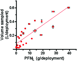
The inclusion of a PFM device when deployed in association with passive samplers can also facilitate the on site assessment of the volume of water extracted over the deployment period at the time of retrieval through the use of a scale where by the distance of the plaster from the container opening corresponds with a approximate volume of water sampled (where ∼23.5 g is equal to 1 cm of plaster height within the PFM). This is demonstrated in Fig. 7 where the calculated volume of water sampled per deployment period (V) by the P-sampler has been plotted against the respective PFM_L. The trend line established is described by Equation 10 and can be used to predict the volume of water sampled with an accuracy of 69%.

V(L) = 0.014 PFM_L + 0.082 (10)

Fig. 7 Volume of water sampled by the P-sampler relative to the total mass lost from the PFM device.

While it is advisable that an accurate prediction of Rs is obtained using Equation 9, the use of Equation 10 will allow the performance of passive samplers to be gauged through the visual assessment of a PFM device while in the field and enable the deployment period to be extended, if necessary, to ensure that a desired volume of water is extracted.

Conclusions

The use of a PFM, a plaster cast, as an in situ calibration device allows a prediction of the effect of flow on the rate of uptake of phosphate (Rs) when the sampling devices are exposed to the flow/turbulence produced by a water velocity of between 3.4 and 24 cm/s. A simple model has been demonstrated to provide a method for the application of a site specific Rs when calculating the environmental concentration of an analyte from the mass accumulated within a passive sampler. The use of this cheap, easy and reproducible in situ external calibration technique enables the use of the P-sampler, a flow dependent passive sampling device to obtain qualitative and quantitative data assuming that the magnitude of flow is relatively constant. Additional work is currently being undertaken to establish the effectiveness of this method under simulated flood conditions when both Cw and water velocity are changing.

Furthermore, the application of the PFM to assess the effects of flow/turbulence and predict site specific Rs is theoretically applicable to all passive sampling devices where the water side diffusion boundary layer influences the uptake of analytes. Further calibrations are currently being performed to investigate the relationship between PFM_L and the uptake of polar and nonpolar organic chemicals into (and PRC loss from) three additional passive samplers, the chemcatcher, polydimethylsiloxane (PDMS) and a semi-permeable membrane device (SPMD). It is anticipated that the results from that calibration will further demonstrate the application of the PFM devices as an additional QCQA method for more accurate and reproducible prediction of chemicals concentrations in water from the mass accumulated in passive sampling devices.

Acknowledgements

The work described was undertaken as a part of an ARC discovery project at the National Research Centre for Environmental Toxicology; UQ and is co-funded by Queensland Health Forensic and Scientific Services (QHFSS).

We thank the contributions of the QHFSS Environmental Water Laboratory for support in the theoretical development of this project. Our appreciation is also extended to the anonymous reviewers of the manuscript for their valuable feedback.

References

1. J. E. Cloern, Mar. Ecol. Prog. Ser., 2001, 210, 223–253.
2. C. Hartog, Aquat. Bot., 1994, 47, 21–28.
3. P. S. Lavery, R. J. Lukatelich and A. J. McComb, Estuarine Coastal Shelf Sci., 1991, 33, 1–22.
4. D. Sanders and R. C. Baron-Szabo, Palaeogeogr. Palaeoclimatol. Palaeoecol., 2005, 216, 139–181.
5. P. Tett, R. Gowen, D. Mills, T. Fernandes, L. Gilpin, M. Huxham, K. Kennington, P. Read, M. Service, M. Wilkinson and S. Malcolm, Marine Pollut. Bull, 2007, 55, 282–297.
6. S. Maritorena, A. Morel and B. Gentili, Limnol. Oceanogr., 1994, 39, 1689–1703.
7. M. S. Thomsen and K. McGlathery, J. Exp. Mar. Biol. Ecol., 2006, 328, 22–34.
8. H. Zhang, W. Davison, R. Gadi and T. Kobayashi, Anal. Chim. Acta., 1998, 370, 29–38.
9. B. Müller, A. Stöckli, R. Stierli, E. Butscher and R. Gächter, J. Environ. Monit., 2007, 9, 82–86.
10. W. Chardon, R. Menon and S. Chien, Nutr. Cycling Agroecosyst., 1996, 46, 41–51.
11. D. S. Baldwin, J. K. Beattie and D. R. Jones, Water Res., 1996, 30, 1123–1126.
12. R. M. Dils and A. L. Heathwaite, Water Research, 1998, 32, 1429–1436.
13. B. Müller, R. Stierli and A. Wüest, Water Resour. Res, 2006, 42, 82–86.
14. X. H. Shao, C. H. Xing, S. T. Du, C. Y. Yu, X. Y. Lin and Y. S. Zhang, Journal of Plant Nutrition, 2006, 29, 1187–1197.
15. W. H. Van Rimesdijk, L. J. M. Boumans and F. A. M. De Haan, Soil Science Society of America Journal, 1984, 48, 537–541.
16. I. R. Willett, C. J. Chartres and T. T. Nguyen, J. Soil Sci., 1988, 39, 275–282.
17. D. Freese, R. Lookman, R. Merckx and W. H. Van Riemsdijk, Soil Science Society of America Journal, 1995, 59, 1295–1300.
18. B. Vrana, I. J. Allan, R. Greenwood, G. A. Mills, E. Dominiak, K. Svensson, J. Knutsson and G. Morrison, TrAC, Trends Anal. Chem, 2005, 24, 845–868.
19. S. Seethapathy, T. Górecki and X. Li, J. Chromatogr. A, 2008, 1184, 234–253.
20. G. Ouyang and J. Pawliszyn, J. Chromatogr. A, 2007, 1168, 226–235.
21. F. Stuer-Lauridsen, Environ. Pollut., 2005, 136, 503–524.
22. J. N. Huckins, J. D. Petty, and K. Booij, Monitors of Organic Chemicals in the Environment. Semipermeable Membrane Devices , 2006, New York: Springer Science + Business Media, LLC, 223.
23. H. Zhang and W. Davison, Anal. Chim. Acta., 1999, 398, 329–340.
24. B. S. Stephens, A. Kapernick, G. Eaglesham and J. Mueller, Environ. Sci. Technol., 2005, 39, 8891–8897.
25. B. Vrana, G. A. Mills, E. Dominiak and R. Greenwood, Environ. Pollut., 2006, 142, 333–343.
26. J. Huckins, J. D. Petty, J. Lebo, F. V. Almeida, K. Booij, D. A. Alvarezda, W. L. Cranor, R. Clark and B. B. Mogensen, Environmental Science and Technology, 2002, 36, 85–91.
27. Y. Arai and D. L. Sparks, J. Colloid Interface Sci., 2001, 241, 317–326.
28. R. Greenwood, G. Mills, and B. Vrana, Passive sampling techniques in environmental monitoring, first ed. Comprehensive Analytical Chemistry, ed. D. Barcelo, vol. 48, 2007, Amsterdam, Elsevier, 453.
29. B. J. Muus, Sarsia, 1968, 34, 61–68.
30. M. S. Doty, Botanica Marina, 1971, XIV, 32–35.
31. A. M. Hart, F. E. Lasi and E. P. Glenn, Aquacult. Eng., 2002, 25, 239–252.
32. R. D. Howerton and C. E. Boyd, Aquacultural Engineering, 1992, 11, 141–155.
33. P. L. Jokiel and J. I. Morrissey, Mar. Ecol. Prog. Ser., 1993, 93, 175–181.
34. T. Komatsu and H. Kawai, J. Oceanogr., 1992, 48, 353–365.
35. E. L. Petticrew and J. Kalff, Can. J. Fish. Aquat. Sci., 1991, 48, 1244–1249.
36. E. T. Porter, L. P. Stanford and S. E. Suttles, Limnol. Oceanogr., 2000, 45, 145–158.
37. D. A. Alvarez, P. E. Stackelberg, J. D. Petty, J. N. Huckins, E. T. Furlong, S. D. Zaugg and M. T. Meyer, Chemosphere, 2005, 61, 610–622.
38. J. K. Kingston, R. Greenwood, G. A. Mills, G. M. Morrison and L. Björklund Persson, J. Environ. Monit., 2000, 4, 487–495.
39. R. B. Schäfer, A. Paschke and M. Liess, J. Chromatogr. A, 2008, 1203, 1–6.
40. V. Kochkodan, S. Tsarenko, N. Potapchenko, V. Kosinova and V. Goncharuk, Desalination, 2008, 220, 380–385.
41. Y.-Q. Wang, Y.-L. Su, Q. Sun, X.-L. Ma and Z.-Y. Jiang, J. Membr. Sci., 2006, 286, 228–236.
42. T. Knoell, J. Safarik, T. Cormack, R. Riley, S. W. Lin and H. Ridgway, J. Membr. Sci., 1999, 157, 117–138.
43. J. Pieracci, J. V. Crivello and G. Belfort, J. Membr. Sci., 1999, 156, 223–240.
44. H. C. Flemming and G. Schaule, Desalination, 1988, 70, 95–119.
45. T. Gorecki and J. Namiesnik, Trends in Analytical Chemistry, 2002, 21, 276–291.
46. R. B. Schäfer, A. Paschke and M. Liess, Journal of Chromatography A, 2008, 1203, 1–6.
47. D. N. Fogg and N. T. Wilkinson, Analyst, 1958, 83, 406–414.
48. C. G. Kowalenko and D. Babuin, Communications in Soil Science and Plant Analysis, 2007, 38, 1299–1316.
49. J. Murphy and J. P. Riley, Analytical Chinica Acta, 1962, 27, 31–36.
50. S.-C. Pai, C.-C. Yang and J. P. Riley, Anal. Chim. Acta., 1990, 229, 115–120.
51. G. Ouyang and J. Pawliszyn, J. Chromatogr. A, 2007, 1168, 226–235.
52. P. S. Nobel, Biophysical plant physiology and ecology, 1983, New York, W.H.Freeman and Company.

---

References

- J. E. Cloern, Mar. Ecol. Prog. Ser., 2001, 210, 223–253 CrossRef CAS.
- C. Hartog, Aquat. Bot., 1994, 47, 21–28 CrossRef.