Online coupling of field-flow fractionation with SAXS and DLS for polymer analysis

Abstract

We report on a hyphenated polymer analysis method consisting of asymmetrical flow field-flow fractionation (A4F) coupled online with small-angle X-ray scattering (SAXS) and dynamic light scattering (DLS). A mixture of six poly(styrene sulfonate)s with molar masses in the range of 6.5 × 10³ to 1.0 × 10⁶ g mol⁻¹ was used as a model system for polyelectrolytes in aqueous solutions with a broad molar mass distribution. A complete polymer separation and analysis was performed in 60 min. Detailed information for all polymer fractions are available on i) the radii of gyration, which were determined from the SAXS data interpretation in terms of the Debye model (Gaussian chains), and ii) the diffusion coefficients (from DLS). We recommend using the A4F-SAXS-DLS coupling as a possible new reference method for the detailed analysis of complex polymer mixtures. Advantages of the use of SAXS are seen in comparison to static light scattering for polymers with radii of gyration smaller then 15 nm, for which only SAXS produces precise analytical results on the size of the polymers in solution.

---

Introduction

Online coupling of asymmetrical flow field-flow fractionation (A4F) and multiangle laser light scattering (MALLS) has been developed by Kulicke et al. for the characterization of dissolved macromolecules and dispersed nanoparticles.^1,2 The great potential of combining A4F and MALLS for the analytical chemistry of polymers has been illustrated for a mixture of sodium poly(styrene sulfonate) (PSS), which is a prototype for macromolecules in aqueous solutions.³ Attainable analytical values are the radii of gyration, R_g, and the diffusion coefficients, D. An A4F-MALLS online coupling allows continuously monitoring of light scattering at different angles and, therefore, R_g can be determined if the sizes of the polymers are larger than λ/20. Unfortunately, the R_g values derived from light scattering deteriorate rapidly for molecules with sizes below λ/20, which means that no reliable R_g values significantly smaller than about 15 nm can be determined when using a typical laser light source with a wavelength of λ = 632.8 nm. In contrast to light scattering, small-angle X-ray scattering (SAXS) uses X-rays with wavelengths of 0.1 to 0.2 nm, and its accuracy for the characterization of dispersed nano-objects with sizes down to 1 nm is well established.⁴ Therefore, SAXS can be substituted for MALLS especially when polymers with R_g < 15 nm are investigated.

Surprisingly, SAXS has not previously been combined with field-flow fractionation methods for the investigation of polymers. This is most probably due to the fact that scattering of visible light by nanosize objects is several orders of magnitude higher than that of X-rays. A priori, one can expect that the SAXS signal of the polymers after field-flow fractionation would be too low to be detected. In a recent study, we circumvented this problem by using a highly intense X-ray source in the form of synchrotron radiation combined with a SAXS system optimized for nanoparticle detection.⁵ It has been shown that the size distribution of the radii (1.2 to 1.7 nm) and lengths (7.0 to 30.0 nm) of superparamagnetic maghemite nanorods can be revealed in situ by the A4F-SAXS coupling. Furthermore, a commercial X-ray tube can also be used for A4F-SAXS when i) strong X-ray scatterers are present, for example, in form of iron oxide nanoparticles and ii) a reduced SAXS data quality is acceptable.⁶

The former investigations were on nanoparticles with very high scattering contrast.^5,6 Our hypothesis was that a A4F-SAXS coupling may also be performed for scatterers with low scattering contrast such as polyelectrolytes in solution, for which the scattering contrast is about 10³ times lower than for dispersed iron oxide nanoparticles. In this context, the objective is therefore to demonstrate in a proof-of-principle study that a mixture of sodium poly(styrene sulfonate)s can be investigated online using A4F-SAXS. It is obvious that a synchrotron is necessary as an intense X-ray source; it is combined with a low sample to detector distance (slit focus system of Kratky type) to produce sufficient scattering intensity. In addition, we complement the A4F-SAXS set-up as used earlier with a differential refractive index detector (RI) for concentration detection of the polymers and dynamic light scattering (DLS) for determination of the diffusion coefficient. A schematic presentation of the A4F-RI-SAXS-DLS setup is shown in Fig. 1. In this context, P is the polymer mixture that is injected in the A4F for fractionation. The fractions were analyzed consecutively online by RI, SAXS and DLS and can be collected afterwards as polymer samples with numbers 1 to N sequentially from low to high molar mass.

Fig. 1 Diagram of the online A4F-SAXS-DLS coupling. The polymer mixture P is injected into the asymmetric flow field-flow fractionation instrument (A4F). The outlet of the A4F is coupled online with i) a differential refractometer (RI), ii) a small-angle X-ray scattering instrument (SAXS) and iii) a dynamic light scattering instrument (DLS). Finally, the fractions of the polymers are collected sequentially from low to high molar mass.

Materials and methods

Materials

Sodium chloride and sodium azide were obtained from Merck. Polymer standards with M_w of 6530, 32900, 63900, 145000, 282000 and 1000000 g mol⁻¹ all with a polydispersity M_w/M_n < 1.2 (determined by GPC/SEC by the manufacturer) were purchased from Polymer Standards Service (PSS).

Methods

Asymmetrical flow field-flow fractionation (A4F). The A4F unit was purchased from Postnova Analytics GmbH (Germany), and consisted of an AF2000 focus system (PN 5200 sample injector, PN 7505 inline degasser, PN 1122 tip and focus pump) equipped with slot outlet technique for increased sensitivity.⁷ An inline solvent filter (100 nm, regenerated cellulose, Postnova) was placed between the solvent pumps (tip and focus) and the channel to reduce the background signals. The channel thickness was 500 micrometers, and the ultrafiltration membrane was a regenerated cellulose membrane with a cutoff of 5 × 10³ g mol⁻¹. A solution of 0.1 M sodium chloride in deionized water with additional 200 mg L⁻¹sodium azide to prevent bacterial growth was used as the solvent for the polymers, as well as for the carrier solution. The latter was filtered through a 0.1 µm regenerated cellulose filter, the samples through a 0.45 µm syringe filter to avoid dust in the samples. The polymer mixture was composed of six sodium poly(styrene sulfonate)s as follows: 7.5 mg mL⁻¹ 6530 g mol⁻¹, 7.7 mg mL⁻¹ 32900 g mol⁻¹, 4.6 mg mL⁻¹ 63900 g mol⁻¹, 5.4 mg mL⁻¹ 145000 g mol⁻¹, 2.6 mg mL⁻¹ 282000 g mol⁻¹ and 1.1 mg mL⁻¹ 1000000 g mol⁻¹. The flow rate was set to 1.0 mL min⁻¹ for the A4F experiment, a slot outlet function was enabled at 80% to reduce further dilution; resulting in a detector flow rate of 0.2 mL min⁻¹. The cross-flow was controlled by AF2000 software from Postnova Analytics. It was set to decrease linearly with time, starting with a flow rate of 2.5 mL min⁻¹, decreasing to 0.2 mL min⁻¹ within 30 minutes and further decreasing to the final cross-flow rate of 0 within 20 minutes according to the power method from Postnova Analytics software AF2000 Control ver.1.1.0.16 with an exponent of 0.5. See also Fig. 2.

Fig. 2 Fractograms of the asymmetrical field-flow fractionation with RI detection of single samples (dashed lines from left to right are from samples p₁ to p₆) and a mixture of six sodium poly(styrene sulfonate)s (solid line). Right axis. Cross flow profile used for elution (dotted line).

A volume of 100 µl of the polymer mixture was injected to the separation channel within five minutes and a further five minute interval of transition time followed before the elution started. The outlet of the A4F was connected directly to the RI detector, the flow cell of the SAXS instrument and the flow cell of the DLS.

Small-angle X-ray scattering (SAXS). SAXS measurements were performed at the BAMline at BESSY II (Berlin, Germany) with a Kratky-type instrument (SAXSess from Anton Paar, Austria) at 25 ± 1 °C. The SAXSess has a low sample-to-detector distance (0.309 m), which is appropriate for investigation of dispersions with low scattering intensities. The measured intensity was corrected by subtracting the intensity of a capillary filled with pure water. The scattering vector is defined in terms of the scattering angle θ and the wavelength λ of the radiation (λ = 0.154 nm): thus q = 4π/λ sinθ. Deconvolution (slit length desmearing) of the SAXS curves was performed with Glatter's established indirect Fourier transformation method^4,8,9 implemented in the PCG Software Version 2.02.05 (University of Graz) to verify the results produced with the SAXS-Quant software.

Dynamic light scattering (DLS). The DLS measurements were performed using a Malvern Instruments particle sizer (Zetasizer Nano ZS, Malvern Instruments, UK) equipped with a He-Ne laser (λ = 632.8 nm). The scattering data were recorded at 25 ± 1 °C in backscattering modus at a scattering angle of 2θ = 173°, which corresponded to a scattering vector of q = 4πn/λsinθ (0.02638 nm⁻¹). The aqueous sample solutions were investigated in a flow through cuvette.

Results and discussion

A quantity of 2.89 mg of a mixture of six sodium poly(styrene sulfonate)s dissolved in 100 µL of 0.1 M sodium chloride was injected into the A4F for separation. The molar masses of the single polymers were M_w = 6.53 × 10³ (p₁), 3.29 × 10⁴ (p₂), 6.39 × 10⁴ (p₃), 1.45 × 10⁵ (p₄), 2.82 × 10⁵ (p₅) and 1.00 × 10⁶ g/mol (p₆). Further details of the polymer characteristics are given in Table 1. The A4F of a polymer sample provides fractions of a narrow polydispersity. We used a mixture of polymer standards to model a very polydisperse sample in order to show the potential of this methodology for polymer analysis. The cross flow gradients used were adjusted for this mixture. Therefore, after 30 minutes of linear cross flow decrease at a rate of 0.076 mL min⁻¹, a period of slow exponential decrease at small crossflow values followed to account for the largest molecules in the mixture (see Fig. 2). A satisfactory fractionation over the entire bandwidth was achieved, which is appropriate for online analysis.

Table 1 Molar mass characteristics of sodium poly(styrene sulfonate)s p₁ to p₆, their fractionation time in A4F, radius of gyration and diffusion coefficient. The M_w/M_n are less than 1.2 for all samples

Polymer	M w (g mol^−1)	m (mg mL^−1)	Elution time (s)	R g (nm)	D (10^−12 m^2 s^−1)
p 1	6.53 × 10^3	7.5	630	1.67 ± 0.01	60–120
p 2	3.29 × 10^4	7.7	780	4.23 ± 0.02	41.7 ± 2.0
p 3	6.39 × 10^4	4.6	1120	6.15 ± 0.03	28.6 ± 1.5
p 4	1.45 × 10^5	5.4	1630	8.44 ± 0.05	20.1 ± 1.0
p 5	2.82 × 10^5	2.6	2100	10.93 ± 0.05	12.2 ± 1.0
p 6	1.00 × 10^6	1.1	2590	22.23 ± 0.10	5.7 ± 1.0

---

After A4F, the fractions were first monitored by the RI detector. The RI signal as shown in Fig. 2 proves that the polymers elute at fractionation times of between 550 and 3000 s. Peaks are visible at 630 and 730 s, followed by a continuous decrease of the signal intensity. The traces of the single poly(styrene sulfonate)s are displayed for comparison in Fig. 2 (dashed lines), where the maxima of the concentration profiles are at 630 s (p₁), 780 s (p₂), 1120 s (p₃), 1630 s (p₄), 2100 s (p₅) and 2590 s (p₆). The shapes of the traces of the individual samples are in good agreement with the trace of the mixture. It should be mentioned that optimized separation conditions were not used. Consequently, a significant lower injection volume (20 to 50 µL) is required, because a sufficiently high polymer concentration to monitor SAXS intensities of good data quality is required, as will be shown later.

Offline determination of the R_g-M_w relation

Prior to A4F, the SAXS patterns of the individual polymers in 0.1 M sodium chloride were measured separately offline for determination of the R_g-M_w relation. The curves of the six individual polymers are displayed in Fig. 3 (solid lines), whereby the intensities are normalized to one at low q for better comparison. It can be seen that the scattering curves of all samples are clearly separated and display the typical shape of well-dissolved polymer chains in diluted solution. No indications of aggregation are present. All curves scale with I(q) ∼ q⁻², which indicates a random coil conformation. The region of I(q) ∼ q⁻² shifts from high to low q-values with increasing molar mass sequentially from p₁ to p₆ as expected (indicated by an arrow). Numerous detailed models are reported for the interpretation of SAXS and small-angle neutron scattering data of poly(styrene sulfonate)s and similar polyelectrolytes with consideration of local, rod-like configuration and counterion condensation.^10–12 Such detailed analysis to find the most appropriate scattering function¹³ and analysis in terms of different worm-like chain models¹⁴ is beyond the scope of the present work. In this paper, we restrict the SAXS data interpretation to the determination of the overall chain dimension as represented by the radius of gyration, R_g. The SAXS of Gaussian chains are given by the Debye function⁴ as

This is a simple two-parameter model in which the shape of the curve is determined only by R_g and I(0) is a intensity scaling factor. We found that the Debye function applies surprisingly well to fitting the SAXS curves in a large q-region resulting in R_g = (1.67 ± 0.01) nm (p₁), (4.23 ± 0.02) nm (p₂), (6.15 ± 0.03) (p₃), (8.44 ± 0.05) nm (p₄), (10.93 ± 0.05) nm (p₅) and (22.23 ± 0.10) (p₆). The corresponding fitted curves are displayed in Fig. 3 (dashed lines). Deviations between data and fitted curve are visible at higher q-values. This is in agreement with a locally rod-like structure where the intensity starts to scale with q⁻¹ on a length scale determined by the persistence length, which is larger for higher molar masses than for lower ones. Nevertheless, the determination of R_g is insensitive to the shape of the curves at high q-values, where details of the polymer structure are visible.

The relation between radius of gyration and molar mass can be used for calibration and also for proving our conclusion of the presence of Gaussian chain conformations. For simplicity, in the following we write R_g instead of 〈R²_g〉^0.5_z. The expected power-law behavior R_g = 〈R²_g〉^0.5_z = k_νM^ν_w is best observed in a double logarithmic plot of R_g as a function of M_w, as shown in the inset in Fig. 3. The parameters as determined from a fit of the data are k_ν = (2.197 ± 0.548) × 10⁻² and ν = 0.500 ± 0.018 (straight line). Within the limits of the experimental uncertainty, the ν-value is equal to the value of a Gaussian chain (ν = 1/2). Therefore, the experimentally determined value of 0.5 is consistent with the applicability of the Debye function for interpretation of the SAXS curves. Kulicke³ determined somewhat different parameters with MALLS (k_ν = 2.71 × 10⁻²and ν = 0.56). Finding of an exponent that is significantly higher than 1/2 means that the polymer chains are more expanded than those of a Gaussian chain. One explanation for the fact that our parameters differ from that earlier study is that the solvent conditions are different, and it is well known that the conformation of poly(styrene sulfonate)s (as for all polyelectrolytes) is strongly dependent on the solvent conditions such as the ionic strength and ionic composition.¹¹

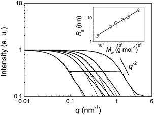Fig. 3 SAXS curves of the six individual sodium poly(styrene sulfonate)s and curve fits using the Debye function (solid and dashed lines, respectively). The arrow points in the direction of increasing molar masses from p₁ to p₆ and increasing radius of gyration with R_g = 1.67 nm (p₁), 4.23 nm (p₂), 6.15 (p₃), 8.44 nm (p₄), 10.93 nm (p₅) and 22.23 (p₆). The straight line indicates a scaling of I ∼ q⁻². Inset: Double logarithmic plot of the radii of gyration as a function of the molar masses (symbols) for determination of the scaling relation R_g = 〈R²_g〉^0.5_z = k_νM^ν_w (straight line). Parameters are k_ν = (2.197 ± 0.548) × 10⁻² and ν = 0.500 ± 0.018.

Online determination of R_g

The knowledge of the M_w-R_g relation from offline SAXS experiments allows a M_w calibration. It should be mentioned that a molar mass determination without this calibration is possible presuming that absolute intensities are measured and the density of the polymers are known.^4,15,16 But this is beyond the scope of this study. In the present study, SAXS intensity detection is performed in arbitrary units. The p₁ to p₆ were detected in a time interval between 600 and 3000 s, which is in good agreement with RI detection. Five examples of SAXS curves at different fractionation times are shown in Fig. 4 (solid lines). We found that the Debye function was suitable for fitting as expected from offline SAXS results. The curves could be fitted over a wide q-range from 0.1 to 2. nm⁻¹ for the fractions with lower fractionation times (Fig. 4, curves a to c). In contrast, the SAXS curves of the fractions with larger fractionation times could only be fitted with the Debye function in the region of low q–values (curves d and e). This is in agreement with a locally rod-like structure where the intensity scales with q⁻¹. But, as mentioned above, this does not affect the determination of the R_g values, which is insensitive to local differences in the chain structure. For typical SAXS curves, the radii of gyration are 1.86 nm at t = 607 s (a), 2.09 nm at 652 s (b), 4.03 nm at 789 s (c), 6.80 nm at 1380 s (d) and 11.80 nm at 2380 s (e) (Fig. 4, dotted lines). The uncertainties of the R_g values from the curve fits are in the range of 0.05 to 0.20 nm.

Fig. 4 SAXS curves at different fraction times (solid lines) and fitted curves using the Debye model (dashed lines). Radii of gyration are 1.86 nm at t = 607 s (a), 2.09 nm at 652 s (b), 4.03 nm at 789 s (c), 6.80 nm at 1380 s (d) and 11.80 nm at 2380 s (e).

An overview of all radii of gyration as a function of the fractionation time is shown in Fig. 5. It can be seen that R_g increases with increasing fractionation time from 1.86 nm at 600 s to about 22 nm 2800 s. This proves that the fractionation by A4F separates the polymer mixture continuously into slices from low to high R_g with increasing fractionation time as expected. It can be seen that the mixture is well fractionated and that the fractions consist of the polymer from p₁ to p₆ as indicated by the horizontal lines.

Fig. 5 The radii of gyration as a function of the fraction time (symbols) resulting from fitted curves with the Debye function as shown in Fig. 4. Horizontal lines indicate the radii of gyration of the polymersp₁ to p₆.

Intersections of the horizontal lines with the R_g curve occur at 607 s (p₁), 789 s (p₂), 1152 s (p₃), 1561 s (p₄), and 2243 s (p₅). The horizontal curve of (p₆) is slightly higher than the R_g values of 18.6 to 22.0 nm found in the interval from 2470 to 2834 s, but it is obvious from the stepwise increase in R_g that p₆ elutes at times larger than 2470 s. These positions on the time scale of these R_g intersections agree very well with the position of the maxima of the RI detection (single traces in Fig. 2). This proves that SAXS allows online detection in combination with A4F for poly(styrene sulfonate)s with a time resolution of 60 s. In addition to the size determination, further information on the polymer structure, which is clearly detected here as random coil, is generated.

The molar masses were determined from the R_g-values using the R_g-M_w calibration, i.e. M_w = (R_g/k_v)^1/ν and displayed as a function of the fractionation time in Fig. 6. It can be seen that the molar mass increases linearly with time for 600 < t < 2500 with a slope of (145.9 ± 2.7) mol g⁻¹ s⁻¹ (straight line). Therefore, the molar mass separation conditions have been optimized for the molar mass range of p₁ to p₅. The value p₆ is not in a line with the others because the cross-flow decrease rate of the A4F changed at 2400 seconds runtime (see Fig. 2) to provide an appropriate separation across the entire range of the sample. For comparison, the M_w-R_g relation is displayed in the inset of Fig. 6. It shows that the slope of the curve is highest below molar masses of 10⁵ g mol⁻¹ and R_g-values lower than 10 nm. The greater the slope the better the possibility to distinguish fractions of different molar masses. This finding confirms our hypothesis that SAXS becomes a valuable method in coupling with field-flow fractionation when the dimensions of the polymers are lower than the λ/20 limit of static light scattering.

Fig. 6 The molar masses as calculated from the R_g values in Fig. 5 for the different times of elution (symbols). The straight line is a curve fitted in the time interval of 600 to 2500 s with a slope of m = 145 g mol⁻¹ s⁻¹. Inset. Relation M_w = (R_g/k_v)^1/νwith k_v = 2.197 and ν = 1/2.

Offline determination of the D-M_w relation

The molar mass dependence of the diffusion coefficient of p₁ to p₆ was measured offline before the online application and the result is shown in Fig. 7. We found that the experimental dependence of LogD on LogM is not strictly linear, a fact which had been observed earlier in a detailed study by Tanahatoe and Kuil.¹⁷ For comparison, we added their values to Fig. 7 (crosses). It can be seen that the values of our two polymers with the highest molar masses (p₅ and p₆) lie below the straight line which results from a curve fit of D = k_dM^d_w with k_d = (7.38 ± 0.18)×10⁻⁹ m² s⁻¹ g⁻¹ mol. From the SAXS results we know that the conformation of the polymers is a random coil. Therefore, we used a constant D–value of 1/2 for curve fitting. Note that the diffusion coefficient of p₁ could not be determined because its molar mass is too low for DLS detection. Measured values of p₁ fluctuate strongly in a range of 60 to 120 × 10⁻¹² m² s⁻¹. But this was expected. When allowing d to adjust during fitting, the values are k_d = (12.48 ± 3.90)×10⁻⁹ m² s⁻¹ g⁻¹ mol and d = (0.548 ± 0.029). Inevitably, the uncertainties of the parameters increase and the higher d-value suggests a more expanded conformation than a random coil. Such an interpretation of an expanded coil conformation has been reported by Tanahatoe¹⁷ (d = 0.61 ± 0.04) and Kulicke³ (d = 0.68) but at slightly different solvent conditions. The diffusion coefficient of a polyelectrolyte is very sensitive to its solvent conditions and concentrations.¹⁸ In addition, the first mode in the DLS intensity correlation function, which is observed at short correlation times, is relatively broad and starts to overlap with the well-known second mode with increasing concentration.¹⁹ Furthermore, D depends strongly on the concentration of a polyelectrolyte. These findings make it difficult to accurately measure diffusion coefficients of polyelectrolytes. Therefore, the D-M_w relation that we determined here must be considered as a first-order approximation in the molar mass range of p₂ to p₆.

Fig. 7 Diffusion coefficient as a function of the molar mass of p₂ to p₆ at a concentration of 1 g L⁻¹ (squares, p₁ is not included). The drawn line is a least square fit for the diffusion coefficient in the form D = k_dM^d_w with k_d = 7.38 × 10⁻⁹ m² s⁻¹ g⁻¹ and a fixed value of d = 1/2. Apparent diffusion coefficients at infinite dilution are from Tanahatoe and Kuil¹⁷ (crosses, not included in the fit).

Online determination of D

The diffusion coefficients were determined online with DLS in series directly after SAXS. Before performing DLS online coupling, it was first determined that the diffusion coefficient is not influenced by the translational flow of the solution in the flow-through cuvette. Results for D in stationary and flowing solutions (0.5 to 2.0 mL min⁻¹) cannot be distinguished in the experimental range of error. In addition, control measurements with standard latex particles with radii of 60 nm and a polydispersity index of 0.05 produce the same values with or without a continuous flow stream. Therefore, we concluded that the time scale of the Brownian motion of the polymer chains is several orders of magnitude more rapid than the time scale of the translational motion from the stream flow through the cuvette. The overlay of the rapid Brownian motion of objects smaller than 60 nm and the slow translational motion of the solution flow are separated widely enough in the DLS intensity correlation function. For our study, the continuous flow of the samples during DLS measurements does not affect the results. This may be different for objects significant larger than 60 nm.

It can be seen in Fig. 8 that the diffusion coefficients decrease with increasing fractionation time. This confirms the result from SAXS that the poly(styrene sulfonate)s are separated sequentially from low to high molar masses. The positions that correspond to the diffusion coefficients as determined by offline DLS are marked as horizontal lines. Points of intersections are at 520 s (p₂), 920 s (p₃), 1100 (p₄), 1900 s (p₅) and 2500 (p₆). These points are approximations of the polymers' fractionation times. But it is obvious from the last chapter that the diffusion coefficients of the poly(styrene sulfonate)s could serve only as a rough estimate for the determination of the fractionation times of the samples. Nevertheless, this demonstrates that DLS can be used online with SAXS and may be of more analytical value, e.g. for polymer core-shell micelles²⁰ or polymer protected inorganic nanoparticles.²¹

Fig. 8 Online measured diffusion coefficients as a function of the fractionation time. Horizontal lines indicate the value of the diffusion coefficients for p₂ to p₆ as measured offline.

Similar to the R_g-M_w-relation, we used the D-M_w-relation to calculate the molar masses as a function of fractionation times as M_w = (D/k_d)^d. The result is shown in Fig. 9 and reflects the correct trend that the molar masses increase with increasing fractionation times. But the M_w values are systematically too high as a consequence of the fact that the accuracy of the D-M_w relation is limited due to the complex behavior of D, which is dependent on numerous solvent parameters.

Fig. 9 The molar masses as calculated from the D values in Fig. 8 for the different times of elution (symbols). Relation for calculation is M_w = (D/k_d)^1/dwith k_d = 7.38 × 10⁻⁹ m² s⁻¹ g⁻¹ mol and d = 1/2.

Conclusions

The online coupling of asymmetric flow field-flow fractionation with small-angle scattering and dynamic light scattering has been demonstrated to be useful to characterize a typical polyelectrolyte, such as poly(styrene sulfonate)s, with a broad molar mass distribution. The time required for online separation plus analysis is approximately one hour. The time resolution for a polymer fraction is 60 s. In addition to the determination of the radii of gyration (from SAXS) and the diffusion coefficients (from DLS), it is possible to attain information on the polymer conformation (e.g. random coil). The method is versatile and can be used for a wide range of polymers with arbitrary molar mass distributions. Strong advantages are seen in comparison to the use of static light scattering for polymer dimensions smaller than 15 nm. In addition, the coupling of SAXS with semi preparative types of field-flow fractionation instruments²² makes it attractive for a wide range of application in polymeric, protein and nanoparticle sciences.

Acknowledgements

The financial support of the Federal Institute for Materials Science and Testing is gratefully acknowledged. We thank H. Riesemeier and R. Britzke for help at the BAMline at BESSY. We also thank S. Rolf and F. Emmerling for experimental support in SAXS and H. Schnablegger for detailed discussions of optimized use of the SAXSess.

Literature

1. D. Roessner and W. M. Kulicke, J. Chromatogr., A, 1994, 687, 249–258.
2. H. Thielking, D. Roessner and W. M. Kulicke, Anal. Chem., 1995, 67, 3229–3233.
3. H. Thielking and W. M. Kulicke, Anal. Chem., 1996, 68, 1169–1173.
4. O. Glatter; O. Kratky. Small Angle X-ray Scattering; Academic Press: London, 1982.
5. A. F. Thunemann, J. Kegel, J. Polte and F. Emmerling, Anal. Chem., 2008, 80, 5905–5911.
6. A. F. Thunemann, S. Rolf, P. Knappe and S. Weidner, Anal. Chem., 2009, 81, 296–301.
7. H. Prestel, R. Niessner and U. Panne, Anal. Chem., 2006, 78, 6664–6669.
8. O. Glatter, J. Appl. Crystallogr., 1977, 10, 415–421.
9. G. Fritz and O. Glatter, J. Phys.: Condens. Matter, 2006, 18, S2403–S2419.
10. K. Kassapidou, W. Jesse, M. E. Kuil, A. Lapp, S. Egelhaaf and J. R. C. vanderMaarel, Macromolecules, 1997, 30, 2671–2684.
11. E. Dubois and F. Boue, Macromolecules, 2001, 34, 3684–3697.
12. M. N. Spiteri, C. E. Williams and F. Boue, Macromolecules, 2007, 40, 6679–6691.
13. J. S. Pedersen and P. Schurtenberger, J. Polym. Sci., Part B: Polym. Phys., 2004, 42, 3081–3094.
14. D. Potschke, P. Hickl, M. Ballauff, P. O. Astrand and J. S. Pedersen, Macromol. Theory Simul., 2000, 9, 345–353.
15. D. Orthaber, A. Bergmann and O. Glatter, J. Appl. Crystallogr., 2000, 33, 218–225.
16. E. Mylonas and D. I. Svergun, J. Appl. Crystallogr., 2007, 40, S245–S249.
17. J. J. Tanahatoe and M. E. Kuil, J. Phys. Chem. A, 1997, 101, 8389–8394.
18. L. X. Wang and H. Yu, Macromolecules, 1988, 21, 3498–3501.
19. M. Sedlak, J. Chem. Phys., 1994, 101, 10140–10144.
20. R. Obeid, E. Maltseva, A. F. Thunemann, F. Tanaka and F. M. Winnik, Macromolecules, 2009, 42, 2204–2214.
21. A. F. Thunemann, D. Schutt, L. Kaufner, U. Pison and H. Mohwald, Langmuir, 2006, 22, 2351–2357.
22. M. Maskos and W. Schupp, Anal. Chem., 2003, 75, 6105–6108.

---