Consensus multivariate methods in gas chromatography mass spectrometry and denaturing gradient gel electrophoresis: MHC-congenic and other strains of mice can be classified according to the profiles of volatiles and microflora in their scent-marks

Abstract

House mice (Mus domesticus) communicate using scent-marks, and the chemical and microbial composition of these ‘extended phenotypes’ are both influenced by genetics. This study examined how the genes of the major histocompatibility complex (MHC) and background genes influence the volatile compounds (analysed with Gas Chromatography Mass Spectrometry or GC/MS) and microbial communities (analysed using Denaturating Gradient Gel Electrophoresis or DGGE) in scent-marks produced by congenic strains of mice. The use of Consensus Principal Components Analysis is described and shows relationships between the two types of fingerprints (GC/MS and DGGE profiles). Classification methods including Support Vector Machines and Discriminant Partial Least Squares suggest that mice can be classified according to both background strain and MHC-haplotype. As expected, the differences among the mice were much greater between strains that vary at both MHC and background loci than the congenics, which differ only at the MHC. These results indicate that the volatiles in scent-marks provide information about genetic similarity of the mice, and support the idea that the production of these genetically determined volatiles is influenced by commensal microflora. This paper describes the application of consensus methods to relate two blocks of analytical data.

---

1 Introduction

The major histocompatibility complex (MHC) is a multi-gene family found in vertebrates, and these highly polymorphic loci encode cell-surface antigen-presenting proteins.¹ Because of their important role in the immune system, MHC genes have been investigated in great depth by immunologists, and increasingly by evolutionary biologists aiming to understand how selection maintains high levels of allelic diversity at MHC loci. MHC diversity is thought to be driven by co-evolving pathogens and parasites; however, another non-exclusive possibility is that sexual selection plays a role.^2–6 Much evidence indicates that MHC genes influence odour and mating preferences in mice,^5–10 which may adaptively function to increase offspring resistance to pathogens and parasites;^5,6 however, it is unclear how MHC genes influence odour. Several mechanisms have been proposed,^9,10 including the ‘microflora hypothesis’, which suggests that MHC genes influence the growth of commensal microbiota that control variation in individual odour.^11,12 This idea is supported by evidence that MHC genes influence commensal microflora in the intestine¹³ and scent-marks¹⁴ of congenic laboratory mice; however, studies examining the odour of animals reared in germ-free environments have produced mixed results.⁹ Some recent studies support the idea that MHC genes influence odour by altering the pool of peptides in the urine of mice (‘the peptide hypothesis’).¹⁵ These mechanisms are not mutually exclusive, and it has been suggested that MHC-bound peptides provide the precursors that are metabolised and made volatile by commensal microflora (i.e. the ‘peptide-microflora hypothesis’).⁹ One of the unsolved questions has been determining whether MHC-dependent microflora might influence urinary volatiles. In this study, we examined how MHC genes influence both microflora communities and volatile compounds in mouse scent-marks, and we applied new methods to analyse these two large and complex datasets. More specifically, we applied a chemometric procedure to compare and examine the microbiological and chemical signals of different strains of mice that vary in their genetic background and MHC-haplotype to answer the following questions:

(1) Can we distinguish (and predict) the genetic strain of a mouse, including strains that differ genetically only at the MHC locus (‘MHC congenics’), using the volatile compounds in scent-marks measured by Gas Chromatography Mass Spectrometry or GC/MS?

(2) Can we also distinguish mouse strains using the microbial communities in scent-marks, using molecular genetic profiles (Denaturating Gradient Gel Electrophoresis or DGGE)?

(3) How does the MHC compare to the rest of the genome (background genes) in its influence on urinary volatiles (GC/MS) and microflora (DGGE)?

(4) Is there a relationship between the pattern of volatiles (GC/MS) and pattern of microflora (DGGE)?

Mouse scent-marks are likely to be multivariate in nature, in that no one single compound is uniquely responsible for the signal – rather like recognising a human face – it is a combination of features that allow for unique recognition. Chemometrics approaches work on multivariate models, that is models taking into account the correlation between the variables, and as such have an important role to play in biology where there are likely to be interactions between variables.

In this study, samples of scent-marks were obtained by inserting glass slides into mouse cages containing a male mouse, which are usually scent-marked by individual mice. This is a form of olfactory communication that provides information about signaller quality to competitors and mates.¹⁶ From these samples of scent-marks, DNA was extracted and the microbial community was genetically fingerprinted using DGGE (16S rRNA gene) to obtain a profile of the commensal microflora,¹⁴ and the chemical profile was analysed using GC/MS after sampling with solid phase microextraction (SPME).

The data analysis procedure began with a feature extraction process where raw microbiological and chemical data were summarized in two distinct data matrices.

Each matrix is composed of sample vectors whose elements identify a set of variables common to all samples in the population, which correspond to the relative intensity of gel bands (DGGE) and the areas of common chromatographic peaks (GC/MS). Following feature extraction, a series of processing steps including scaling, normalization and standardisation are applied in order to maximize the interpretability of the information embedded in the matrices. The last part of the procedure involves a variety of multivariate pattern recognition techniques to extract the information of interest from the processed data with which to answer the relevant questions. The main trends emerging from the two blocks are investigated using Consensus Principal Components Analysis (C-PCA)^17–19 that identifies the common directions of variation and can be posed in relation to factors of interest such as background genetics and MHC-haplotypes of mice. The exploratory analysis is then completed with an estimation of the degree of overlap between the microbiological and chemical profile to verify the microflora hypothesis. Afterwards, other techniques such as Partial Least Squares Discriminant Analysis (PLS-DA)^20–24 and Support Vector Machines (SVM)^25,26 were applied to determine whether the fingerprint recorded can be used for prediction purposes. Results indicate that the mouse strains emerge clearly in both profiles recorded and that this information can be used to produce predictive models. The strains of the mice contribute to shape both the GC/MS and DGGE profiles, with the whole strain differences having a stronger effect than MHC. Finally the profiles show a certain degree of overlap.

2 Experimental

2.1 Animals

Twenty-eight male congenic mice from four strains (two MHC-congenic strains) were obtained from Harlan UK: BALB.B/OlaHsd (strain BALB/c, MHC-haplotype b), BALB/cOlaHsd (strain BALB/c, haplotype d), C57BL/10ScSnOlaHsd (strain B10, haplotype b) and C57BL10.D2/nOlaHsd (strain B10, haplotype d). Mice were single-housed in MB2 (20 × 10 × 13 cm) cages in mixed strain racks and maintained under controlled temperature (17–28 °C) and light conditions (reversed 12 h : 12 h light : dark cycle with lights on at 22:00 hours), with ad libitum access to water and food (SDS rat and mouse breeding diet RM3 (P), Special Diet Services, Witham, Essex, UK), shredded paper nesting material and cardboard tubes and softwood chewing sticks for enrichment. Scent-marks were collected when the mice were aged 14–23 weeks.

2.2 Scent-mark collection

Glass microscope slides (76 × 26 × 1.5 mm thick) were frosted on one side using an abrasive, silicon carbide (Carborundum), and cut into two strips each measuring 76 × 13 mm. They were cleaned with a specialist glass cleaner (Dri-Decon), rinsed in tap water and oven-dried overnight at 110 °C. For scent-mark collection, three strips of frosted glass slide were placed frosted side up on a clean glass slide (76 × 38 × 1.5 mm thick) resting on a foam pad (76 × 38 × 5 mm thick) on an upside-down aluminium mini bread tin (10 × 5.4 × 3.2 cm deep). A second mini bread tin with a square hole (65 × 30 mm) cut out was placed on top to hold the slides in place. This device raised the area to be scent-marked 4.4 cm above the substrate, reducing the contamination by materials from the cage bottom. The device was placed in a mouse cage for scent-mark collection for 1.5 h at the beginning of the dark phase (i.e. the animal's active period). The slides were then removed from the metal holders, placed in a silanised 40 ml EPA glass vial with a polypropylene (PP) screw cap and a Silicone/PTFE septum and stored in a freezer at −80 °C. The vials were further stored in 32 oz glass jars with a solid PP Teflon-lined cap to limit contaminants such as CO₂ penetrating the septum. Vials were silanised in order to reduce the adhesiveness of the glass surface with a 2% solution of dichlorodimethylsilane in chloroform, left in a fume cupboard overnight, rinsed in tap water and dried for a minimum of 3 h at 110 °C. After scent-mark collection, the metal tins and clear glass slides were hand-washed and the foam pads machine-washed at 60 °C with Dri-Decon and left to dry overnight on top of a 110 °C oven.

2.3 SPME fibre

Volatile compounds were extracted from scent-marks with a Solid Phase Micro Extraction (SPME) procedure. In order to assess the recovery and sensitivity of different fibre types with our sample of interest – mouse scent-marks – five commercially-available types were compared by exposure to identical samples. All SPME fibres were supplied by Supelco (Bellefonte, PA) and were pre-conditioned by inserting them into the GC injector according to the manufacturer's instructions. As the amount of analytes in real scent-marks was not constant and not controllable over time, simulated scent-marks were used. These were prepared by injecting 10 µl mouse urine onto clean frosted glass strips which had previously been sealed in an EPA glass vial. Ten µl urine gave a comparable GC/MS signal to that of authentic scent-marks. Sampling was done at 60 °C for 30 min in order to maximize recovery and the number of peaks. A total of 107 volatile compounds was detected, although no fibre detected all compounds. The SPME fibre that recovered most volatiles (95 peaks) was a 50/30 divinylbenzene/Carboxen on PDMS and was employed in further analysis.

2.4 Chemical analysis

Immediately before SPME sampling, 2 µl methanol solution containing the internal standards fluorobenzene (8 ng), toluene-d₈ (8 ng), 4-bromofluorobenzene (8 ng), 1,2-dichlorobenzene-d₄ (8 ng) and hexanoic acid-d₁₁ (40 ng) was injected onto the scent-marked collecting materials. The air-tight glass vial was mounted onto a magnetic stirrer and submerged in a 60 ± 1 °C water bath. It was imperative that the scent-marked glass strips remained separated in the vial to avoid impeding the release of volatiles into the headspace. The headspace of the vial was sampled for 60 min (unless indicated otherwise) with the SPME fibre exposed from the protective needle by pushing the plunger forward of the manual holder. After sampling, the fibre was retracted and the needle was removed from the vial. The SPME needle was then inserted into the GC injector and the fibre was exposed to the carrier gas by pushing the plunger of the manual holder. The analytes were thermally desorbed for 3 min in the hot GC injector. The analysis of all extracts was performed on an Agilent 6890N Gas Chromatograph coupled to a 5973 inert Mass Selective Detector (Agilent Technologies, Stockport, UK). The technical specifications of the GC capillary column was: Zebron, ZB-Wax, ∅ 0.25 mm × 30 m, film thickness 0.25 µm, 100% poly(ethylene glycol) (Phenomenex UK Ltd, Macclesfield, UK). The GC injection port liner used was an SPME injection sleeve of 0.75 mm ID (Supelco, Bellefonte, PA). The carrier gas used was helium. The injector temperature was 230 °C in a pulsed splitless mode at a pulse pressure of 25 psi for 2 min. After 2 min, carrier gas was introduced at a constant flow at 1.00 ml min⁻¹. The 69 min oven temperature ramp program was: 40 °C (hold for 5 min), then to 100 °C at 3 °C min⁻¹ (5 min) followed by to 150 °C at 5 °C min⁻¹ (5 min), and finally to 230 °C at 5 °C min⁻¹ (8 min). The spectrometer was run with the following parameters: positive electron ionization mode (EI+), source energy 70 eV, full scan in the mass range of m/z 35–400 amu, no solvent delay, interface transfer line 250 °C. The detector signals were collected, integrated and recorded using an MSD Chemstation (Agilent Technologies).

2.5 Microbiological analysis

DNA was extracted from the glass slides using the Fast Prep DNA SPIN kit (Anachem) with modifications. Glass slides were rotated at room temperature with the cell suspension and cell lysing buffer for 30 min after which the nucleic acids were extracted as described by the manufacturer. The low amounts of DNA recovered from the samples necessitated that all samples were amplified twice with polymerase chain reaction (PCR).¹⁴ Mouse-specific, 16S rRNA gene sequence profiles were produced by separation of the heterogeneous PCR products using DGGE, which was performed using the DCode system (Bio-Rad, Hercules, CA, USA) as described previously.²⁷ A reference marker, constructed using clones of marker bacteria, was included on each gel to verify the continuity of the gradient and to facilitate comparison between patterns. Gels were stained for 1 h in 1X TAE buffer containing Sybr-Green (molecular probes) prior to digitization.

2.6 Computation

All computations were performed on a PC desktop Dell Dimension 2400, 2.20 GHz, 1 GB Ram, with Matlab 6.5 (Mathworks) using in-house software. SVM was applied using the OSU-SVM ver. 3.00 Toolbox by Maet al.²⁸

3 Chemometric methods

Experiments are setup in a way to compare odours from mice that vary systematically in their genetic background and MHC-haplotype. The dataset is composed of four distinct groups of samples as follows: (i) strain BALB, MHC-haplotype H-2^d; (ii) strain BALB, MHC-haplotype H-2^b; (iii) strain C57BL10, MHC-haplotype H-2^d; and (iv) strain C57BL10, MHC-haplotype H-2^b. Hereafter, these groups will be referred as to S₁H₁, S₁H₂, S₂H₁ and S₂H₂ respectively. This design allows comparing mice with same genetic background but different MHC-haplotype (S₁H₁vs. S₁H₂; S₂H₁vs. S₂H₂) as well as mice with different genetic background but with same MHC-haplotype (S₁H₁vs. S₂H₁; S₁H₂vs. S₂H₂).

Chemical and microbiological data are both acquired for 34 mice (dataset α) divided in the four groups indicated above (9 S₁H₁, 9 S₁H₂, 8 S₂H₁ and 8 S₂H₂). In addition, further GC/MS analysis is carried out on another 58 mice (dataset β, 13 S₁H₁, 11 S₁H₂, 15 S₂H₁ and 17 S₂H₂). These two datasets are used for two different purposes. Dataset α allows an initial exploration of the data, where main trends can be searched for after merging the microbiological and chemical information and can be subsequently posed in relation to the genetics of mice, i.e. their strain as well as MHC-haplotypes. A consensus analysis enables to verify which measure in each block contributes to the patterns in the data and most importantly whether and to what extent, similar trends are reproduced in the microbiological and chemical profile. This may provide clues to verify the possible shaping of the commensal microflora by the MHC-haplotypes.

Dataset β, which consists of more instances, can be used to build up a statistical model to verify whether the chemical profile can be used to predict the genetics of mice. Dataset β will train a classifier that will be tested on the instances of dataset α.

3.1 Feature extraction

The purpose of this operation is to extract from the raw data a defined number of variables for each sample to arrange into two distinct data matrices that will summarize the information obtained by the chemical and microbiological analyses. Each sample must be described by the same number of variables and each variable must refer to the same entity across all samples. This preparation phase is necessary for most analytical techniques and can be more or less laborious depending on the characteristics of the data.²⁹

In DGGE, the variables correspond to the intensities of the bands identified along the gel. Feature extraction is straightforward as it requires a digitization of the image of the DGGE gel (Bionumerics gel analysis software, Applied Maths, Sint-Martens-Latem, Belgium) where lanes are aligned relative to internal markers and the intensity of the bands is measured and quantified.^30,31

For GC/MS, variables correspond to the areas of the peaks having a common chemical origin in different chromatograms of all samples^32,33 to form peak tables. Although faster alternatives are available for data screening (e.g. using Total Ion Currents or Single Ion Chromatograms), this method is preferred because it directly relates to the chemical components in the mixture, hence making feasible the identification of potential marker compounds in a subsequent phase of the analysis. However, the procedure is laborious, particularly because chromatograms may contain several hundreds of compounds per sample, the signal-to-noise ratio may be low, and peaks may partially overlap, so peaks must be compared on the basis of their spectral and retention characteristics. The procedure involves four main stages and the basis of the first three steps is described in detail elsewhere³⁴ and takes advantage of the MS information to align peaks in different chromatograms and form a peak table. The main steps are summarized below.

(1) Smoothing of single ion chromatograms. Noise is smoothed with a DB5 (Daubechies wavelet) wavelet filter and three levels of decomposition, chosen based on the data under investigation: because the data contain a significant amount of high frequency noise which is caused by the column (high bleeding) such a wavelet appeared to be the most effective one with very little distortion.

(2) Determining the position and intensity of peaks. Next the first derivative is calculated using a Savitzky–Golay five-point quadratic filter.³⁵ The profile is then processed using a switch-position loop. A peak start is taken as whenever the first derivative becomes positive. A peak maximum is taken when two sequential first derivative points are negative and either the peak is at least seven datapoints wide or the peak is at least four times higher than the lowest non-zero value in the chromatogram. The second criterion is necessary to detect partially overlapped peaks found on the shoulder of other peaks that are not sufficiently large. A peak end is taken as when two sequential first derivative points are positive. This step is performed on all the mass ions and peaks with same retention time for different ions are then merged together. The combination of their intensity is used to estimate their area while the combination of ions is assigned as the spectrum of the compound. The procedure is then applied on all samples and the dataset matrix is deduced by means of a pair-wise comparison of peaks across samples on the basis of their spectral profile. The intensity of peaks is determined by our previously published method.³⁴

(3) Matching peaks from a common origin. The procedure starts from the first peak of the first sample, looking for peaks within a defined retention time window across the second sample. If a peak with a similar MS is found, the areas are allocated in the same column of the matrix (same variable), otherwise the unmatched peak is regarded as originating from a new compound and is placed in a new column and assigned as a new variable. The procedure is repeated for all peaks detected in all samples. Various further failsafe mechanisms are incorporated into our method.³⁴

(4) Removing rare peaks. Because a number of unique peaks are detected in only a small portion of samples and have low diagnostic power for a class, only those detected in at least four samples are retained for further analysis.

3.2 Pattern recognition

After the signal processing step described above, the microbiological and chemical information acquired with DGGE and GC/MS is summarized in two distinct matrices (X_M and X_C). Both are composed of 34 row vectors (samples of dataset α) with 30 and 780 variables respectively, corresponding to different gel bands and chromatographic peaks.

A series of additional processing steps must be applied to make the application of the following pattern recognition techniques for exploration and classification effective. It is desirable to scale the data using a logarithmic transformation in order to reduce the influence of large peaks, and to reflect the fact that intensities are often log-normally distributed. However, an additional problem then relates to the sparseness of X_M and X_C, as both matrices contain a relatively high proportion of zeros because some bands and peaks are found only in a portion of the samples: we find in many areas of metabolomic profiling that marker peaks are present only in a portion of samples. In order to compute logarithms of the peaks that are either absent or below the detection we replace the zeros with half of the lowest intensity peak detected in the dataset. Next, each sample is normalized along rows so that the sum of variables equals one: this allows maximizing the comparison between samples, removing unwanted effects such as the quantity of material sampled and analysed. Finally data are standardised along columns to attribute to each variable an equal weight.

3.2.1 Consensus analysis. A well known technique for visualising multivariate data is Principal Components Analysis (PCA).^36,37 Although PCA operates in an unsupervised manner, as any information on the class membership is not provided, in this application the interpretation of the derived plots is simplified by the fact that the system investigated is well controlled. Mice are housed under the same conditions, and so environmental sources of variation should be randomized among the strains of mice.

In the last few years, modifications of the PCA have been introduced to break the descriptors into several blocks to improve the interpretation of the models, one of which is consensus PCA (C-PCA).^18,19,38 In our case it is initially of interest to verify what is the ‘consensual’ view obtained from merging the information available from X_M and X_C and to determine what is the contribution of each of the two profiles. In C-PCA, the data matrix X is broken down in different blocks (X_C and X_M in our case) and a consensus direction among all the blocks is sought. The method starts by selecting a super-score t that is multiplied on all blocks to give the block loadings. The block loadings are normalized to length one and then multiplied through the respective blocks to give the block scores. The block scores are combined in the super-block T. Then a PCA iteration on T is performed to give the super-weight w^T that is normalized to length one and multiplied onto the super-block T to obtain an improved estimate of the super-score t. This is repeated until convergence of t. The super-score T summarizes the main trends between all blocks and block scores T_M and T_C represent the individual contribution of each block that are related to the former by means of the weight vector w (Fig. 1). The algorithm adopted here is the one originally proposed that incorporates a block-scaling to balance the contribution of X_C and X_M relative to the number of variables. In addition, to stabilise the algorithm, the super-scores are initialised as suggested¹⁸ with the first score vector calculated from the super-matrix determined as follows:

where m is the number of variables in X_M (30 gel bands) and c is the number of variables in X_C (780 chromatographic peaks of unique origins). The super-scores can be visually inspected to determine the consensus view provided by both blocks and can be compared to block scores that will contribute proportionally to their weights. In addition to obtaining a consensual view, it is of interest to determine whether and to what extent the two blocks X_M and X_C directly relate to each other. The amount of correlation between the matrices can be calculated using the RV coefficient:³⁹
where tr indicates the trace of the matrix. The coefficient is standardised, i.e. it spans the interval [0,1] and returns 1 in case of perfect correlation. In addition its value is invariant to scaling and rotation, therefore the coefficient can be effectively used also on the super-space extracted with PCA, to measure to what extent the configurations derived give the same view of the samples. This solution may be preferred to comparing directly X_M and X_C because PCA reduces the data-space of the blocks to their essential variability, smoothing out the noise present in X_M and X_C.

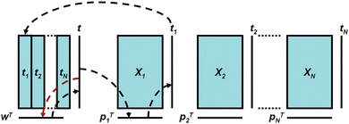Fig. 1 Principles of C-PCA. The scores obtained from each data-block t₁…t_N, are joined into a matrix from which a super-score is extracted to describe the overall trend in the data.

3.2.2 Prediction. After the identification of the main trends and patterns in the data, it is of interest to determine whether the information acquired can be used to predict the origin of new samples, i.e. the genetics (MHC and strain) of the mice analysed. In this sense, the information recorded would act as an effective fingerprint to perform recognition. Classification is attempted using the chemical data only, for which additional data (dataset β) of 58 scent-mark samples analysed by GC/MS are available.

The first technique used is PLS-DA. SVM is used as an alternative in its basic form (LIN-SVM) and with a radial basis kernel (RBF). Further details about SVMs are discussed elsewhere.^25,26,40

The optimal parameters of the model (number of components for PLS-DA, penalty error C for LIN-SVM, C and radial width σ for RBF-SVM) are determined by a leave-one-out procedure: a model with a certain parameter setting (i.e. a given number of PLS components for PLS-DA or kernel parameters, i.e.C and σ, for SVM) is built using 57 of the 58 samples of dataset β and its prediction ability tested on the sample left out, with the procedure repeated for each sample. For PLS-DA, the number of PLS components varied from one to ten and for SVM, C and σ were varied according to a grid search procedure. The parameters of the best model, i.e. the one with the lowest error rate, is then used to build the predictive model on the full dataset β and this model was tested on the 34 samples that compose dataset α.

4 Results and discussion

The feature extraction procedure summarizes the information recorded by DGGE and GC/MS into two data matrices X_M (34 × 30) and X_C (34 × 780). The DGGE matrix is illustrated in Fig. 2. The relatively low number of variables in X_M allows a direct visual inspection where it appears clearly the presence of bands related to the strains, e.g. band nos. 1 and 27 for S₁ as well as band nos. 18, 19 and 21 for S₂. To a minor extent, bands characteristic of the MHC are also observable, e.g. band no. 14 for H₂ and band no. 15 for H₁. The higher dimensionality of X_C does not allow drawing such direct conclusions on the second block of data, hence requiring multivariate modelling to summarize the main trends.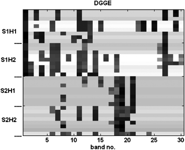

Fig. 2 DGGE (X_M) matrices obtained by feature extraction.

4.1 Exploratory analysis

Consensus PCA is applied on both blocks X_M and X_C to extract the consensual view on the samples of dataset α (Fig. 3). The first two super-scores (on the top) indicate a main trend that directly relates to the strain membership. S₁ samples are located towards the left of the plot (filled-in symbols), while the S₂ samples (open symbols) distribute in a rather compact cluster in the top right quadrant. A less pronounced distinction can also be detected in relation to MHC, where H₁ samples (circles) and H₂ samples (triangles) tend to separate along the top right–bottom left diagonal. The related block scores plots for X_M and X_C exhibit a similar distribution, although X_C is characterised by a higher dispersion. Fig. 4 shows the norm of the super-scores (top), indicating that the first two are in fact predominant and describe a large portion of the data-blocks. The weights (bottom) indicate that X_M is explained well by the first two super-scores, while X_C contributes more to the following components. In addition, with some overlap, the third and fourth super-scores (Fig. 3, bottom) further indicate a trend relating to MHC, with samples partially separated again along the top left–bottom right diagonal. In addition, S₂ samples seem to be somewhat less dispersed as they distribute closer to the centre of the plot, hence explaining less variation. Also, the blocks scores in these two components appear more markedly different from each other.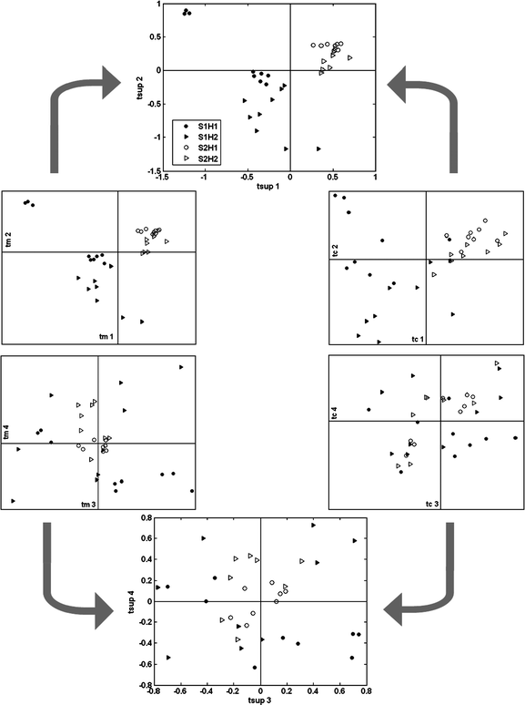

Fig. 3 C-PCA. The scatter plot of super-scores t_sup (middle) are derived from the scores t_m of block X_M (on the left) and the scores t_c of the block X_C (on the right). Symbols for the four groups S_nH_n where n = 1 or 2 are defined in the top graph.

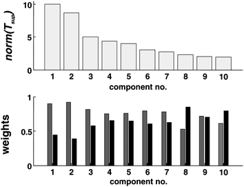Fig. 4 Size of the super-scores t_sup (top) and weights of the block scores (bottom) t_m (grey) and t_c (black).

Whereas supervised feature selection could be performed to obtain better apparent graphical separation between the groups, such supervised methods can lead to overfitting of the data and are only legitimate if one is sure in advance that there will be a separation. It can be shown⁴¹ that using a completely random dataset, by choosing the variables that appear most diagnostic, apparently good separation can be obtained. In hypothesis-based biology, it is often dangerous to perform supervised feature selection prior to graphical visualisation of results, although legitimate to simplify the data using criteria unrelated to the hypothesis being studied; for example, we remove rare variables from the dataset that occur in less than four samples.

Summarizing, the results indicate that the genetic strain of the mice influences the composition of the commensal microbiota from scent-marks as well as the volatile compounds, with a stronger trend associating to the strain membership and a weaker but clearly visible trend associating with MHC-haplotype. Nevertheless, the weights (Fig. 4, bottom) for the chemical data suggest that a substantial amount of variation is not explained by these factors. This is further confirmed when calculating the amount of overlap between X_M and X_C, with the RV coefficient having a value of 0.47. The correlation value substantially increases when the blocks are reduced to their essential variability using the scores of the principal component space. Fig. 5 shows where the RV coefficient exceeds a value of 0.65 for each possible combination of the PCs. Each subset combination of PCs is considered because factors of higher order may relate to trends in the data that are unique for a block (e.g. instrumental drift in GC/MS), hence affecting the correlation negatively. It is possible to observe that the first two components are well correlated and PC2 from X_M resembles PC2, PC3 and PC4 from X_C. The correlation rises to a maximum of 0.84 for the configurations given by the first two PCs of both X_M and X_C. The matrices X_M and X_C show a degree of overlap, but also have a substantial variation that is specific to each block. This is expected, particularly for X_C, where the matrix is composed by several hundred variables and may result in a richer and more complex pattern. Systematic variations that effect solely either X_M or X_C may decrease the amount of correlation. Examples may be the occasional presence of contaminants during the sampling phase or instrumental drift. In addition, it can be noticed that some genetically related factors may contribute to the distribution of only one of the two blocks, for example, volatiles that that do not interact with the metabolism of the microflora, or in turn, MHC-induced chemicals that interact with the microflora but that the sampling technique combined with GC/MS is unable to determine.

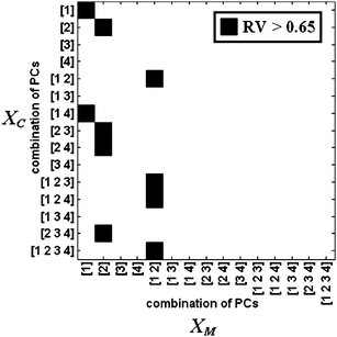Fig. 5 Map of the RV coefficients.

The identification of potential chemical markers in X_C relating to genetics can be readily carried out looking at the block loadings (Fig. 6). In PCA, the loadings represent the weights of the original variables in determining the block scores as illustrated in Fig. 3. Relevant variables for a given group observed in the plot of the scores locate in an analogous axis position in the loadings plot. It was observed that the block scores of the first two components allow a separation between S₁ and S₂ along the top left–bottom right diagonal and a (milder) separation between H₁ and H₂ along the bottom left–top right diagonal. Some potential markers, located at the extremes of such directions in the loadings plots are taken and their quantitative distribution examined in Fig. 7. Peak nos. 458 and 74 display a distribution consistent with S₁ and S₂ respectively, while peak nos. 534 and 528 are related to H₁ and H₂. The mass spectra of these four compounds are presented in Fig. 8.

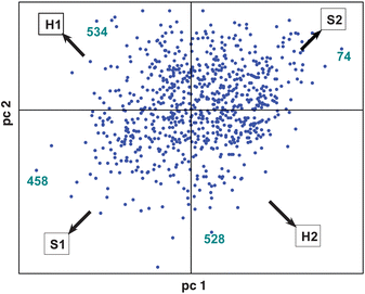Fig. 6 Block loadings of X_C.

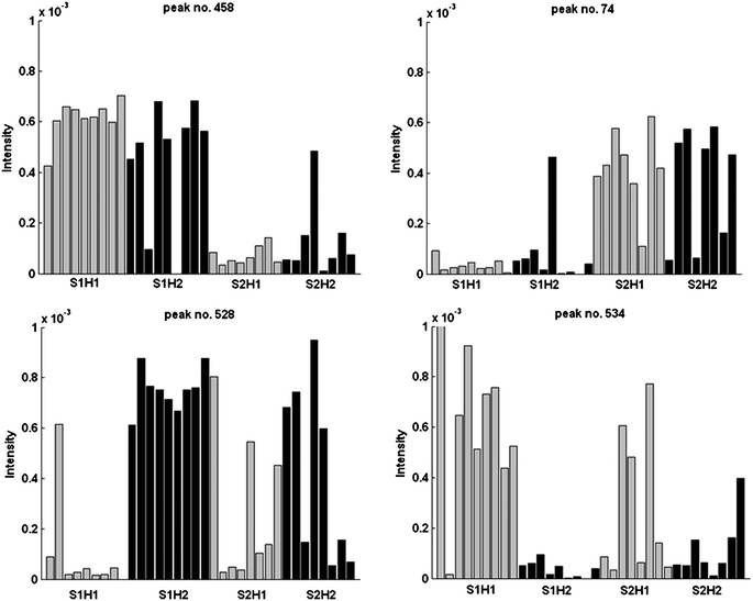Fig. 7 Potential markers for MHC and strains in the GC/MS data.

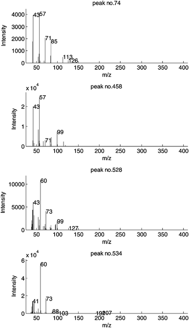Fig. 8 Mass spectra of four potential marker peaks.

4.2 Classification

The use of the chemical information as a fingerprint to predict genetics is summarized in Table 1. Optimisation with a leave-one-out procedure leads to the selection of a PLS-DA model with two components for strain classification and three components for haplotypes. The optimal value of the penalty error for LIN-SVM is C = 0.01 both for strains and haplotypes. For RBF-SVM, optimisation returns C = 50, σ = 0.01 for strains, and C = 100, σ = 0.0005 for haplotypes as models.

Table 1 Classification performance of SVM and PLS-DA

Correct classification (%)					ID misclassified samples
	Training set		Test set
	Strains	Haplotypes	Strains	Haplotypes	Strains	Haplotypes
LIN-SVM	100	100	97.06	88.24	No. 23	Nos. 2, 3, 12, 34
RBF-SVM	100	100	100.00	85.29	N/a	Nos. 2, 3, 4, 12, 34
PLS-DA	92.86	100	97.06	85.29	No. 34	Nos. 2, 14, 18, 28, 34

---

All three classifiers perform very similarly, with no substantial differences. Auto-prediction on the samples of dataset β, which were used to build the model, returns a perfect classification. Most notably, testing on a separate dataset α indicates that strain membership (genetic background) can be better predicted than haplotype membership (MHC-haplotype). However, a rate of 85–88% for classifying by MHC-haplotype further indicates that this feature is consistently present in the data and can be implemented to generate a predictive model that performs satisfactorily.

5 Conclusions

Our goals were to examine whether the volatile compounds (analysed by GC/MS) or microbial communities (analysed with DGGE fingerprinting) in scent-marks differ among strains of mice, and if so, whether there are any relational features between the two extended phenotypes. Further, we examined the effects influenced by MHC-genes as well as the whole genetic background (i.e. the entire genome excluding the MHC region). The experimental design allowed us to compare the effects of MHC genes with those of the whole genetic background (i.e. the entire genome excluding the MHC region), while controlling environmental sources of variation (e.g. diet, social conditions, etc.). To our knowledge, this is one of the first studies to provide evidence that MHC and other genes influence the composition of volatile compounds in urine (and the first analytical study on scent-marks),^7,8 and it is the first study to simultaneously compare the patterns of volatiles with microflora communities.

The raw data analysed with DGGE and GC/MS are organised by means of a feature extraction process in two distinct matrices X_M (DGGE) and X_C (GC/MS) that can be multivariately modelled. Consensus PCA shows that the genetic background (S₁ and S₂, Fig. 3) has a strong influence in shaping both X_M and X_C but a milder trend is clearly observable also in reference to the MHC-haplotype. Matrix correlation analysis indicates that X_M and X_C are partially correlated, but also bring consistent complementary information. These findings are associations, and further experimental manipulations are necessary to determine whether genetics influences individual microflora in scent-marks, and whether these influence profiles of volatile compounds.

Classification by means of PLS-DA and SVM demonstrates that the chemical signatures in scent-marks provide a surprisingly effective fingerprint for predicting mouse strain, as we found that the strains are perfectly classified, and MHC-haplotypes were also predicted with high accuracy.

Acknowledgements

Alexandra Katzer, Dr Penn's administrative assistant, is thanked for her superb organisational skills. This work was sponsored by ARO Contract DAAD19-03-1-0215. Opinions, interpretations, conclusions, and recommendations are those of the authors and are not necessarily endorsed by the United States Government. This work is approved for public release, distribution unlimited.

References

1. D. J. Penn and P. Ilmonen, Encyclopedia of Life Sciences, Macmillan, London, 2005.
2. D. J. Penn and S. Fischer, The Biologist, 2004, 51, 207–211.
3. K. Yamazaki, E. A. Boyse, V. Mike, H. T. Thaler, B. J. Mathieson, J. Abbott, J. Boyse, Z. A. Zayas and L. Thomas, J. Exp. Med., 1976, 144, 1324.
4. C. Wedekind, T. Seeback, F. Bettens and A. J. Paepke, Proceedings of the Royal Society of London Series B-Biological Sciences, 1995, 260, 245.
5. D. J. Penn, Ethology, 2002, 108, 1.
6. D. J. Penn and W. K. Potts, Am. Nat., 1999, 153, 145.
7. M. V. Novotny, H. A. Soini, S. Koyama, D. Wiesler, K. E. Bruce and D. J. Penn, J. Chem. Ecol., 2007, 33, 417–434.
8. A. Willse, A. M. Belcher, G. Preti, J. H. Wahl, M. Thresher, P. Yang, K. Yamazaki and G. K. Beauchamp, Anal. Chem., 2005, 77, 2348.
9. D. J. Penn and D. W. Potts, Adv. Immunol., 1998, 69, 411.
10. K. Yamazaki, K. A. Singer and G. K. Beauchamp, Genetica, 1998, 104, 235.
11. K. Yamazaki, G. K. Beauchamp, Y. Imai, J. Bard, S. P. Phelan, L. Thomas and E. A. Boyse, Proc. Natl. Acad. Sci. U. S. A., 1990, 87, 8413.
12. H. M. Schellinck, E. Rooney and R. E. Brown, Phys. Behav., 1995, 57, 1005.
13. P. Toivanen, J. Vaahtovuo and E. Eerola, Infect. Immun., 2001, 69, 2372.
14. C. V. Lanyon, S. P. Rushton, A. G. O'Donnell, M. Goodfellow, A. C. Ward, M. Petrie, S. P. Jensen, L. M. Gosling and D. J. Penn, FEMS Microbiol. Ecol., 2007, 59, 576.
15. T. Leinders-Zufall, P. Brennan, P. Widmayer, P. Chandramani, A. Maul-Pavicic, M. Jager, X. H. Li, H. Breer, F. Zufall and T. Boehm, Science, 2004, 306, 1033.
16. L. M. Gosling and S. C. Roberts, Advances in the Study of Behaviour, 2001, 30, 169.
17. S. Wold, S. Hellberg, T. Lundstedt, M. Sjöström and H. Wold, Proc. Symp. on PLS Model Building: Theory and Application, Frankfurt am Main, 1987.
18. J. A. Westerhuis, T. Kourti and J. F. MacGregor, J. Chemom., 1998, 12, 301.
19. A. K. Smilde, J. A. Westerhuis and S. de Jong, J. Chemom., 2003, 17, 323.
20. S. J. Dixon, Y. Xu, R. G. Brereton, A. Soini, M. V. Novotny, E. Oberzaucher, K. Grammer and D. J. Penn, Chemom. Intell. Lab. Syst., 2007, 87, 161.
21. B. K. Alsberg, D. B. Kell and R. Goodacre, Anal. Chem., 1998, 70, 4126.
22. R. G. Brereton, Applied Chemometrics for Scientists, Wiley, Chichester, 2007, ch. 10.
23. M. Sjöström, S. Wold and B. Söderström, in Proceedings of PARC in Practice, Elsevier Science Publishers, Amsterdam, 1985.
24. L. Ståhle and S. Wold, J. Chemom., 1987, 1, 185.
25. Y. Xu, S. Zomer and R. G. Brereton, Crit. Rev. Anal. Chem., 2006, 36, 177.
26. V. N. Vapnik, The Nature of Statistical Learning Theory, Springer, New York, 2nd edn, 2000.
27. G. Muyzer, E. C. de Waal and A. G. Uitterlinden, Appl. Environ. Microbiol., 1993, 59, 695.
28. J. Ma, Y. Zhao and S. Ahalt, Ohio State University, OSU SVM Classifier Matlab Toolbox ver 3.00, http://www.ece.osu.edu/%7Emaj/osu_svm.
29. R. O. Duda, P. E. Hart, D. G. Stork, Pattern Classification, Wiley Interscience, New York, 2nd edn, 2001.
30. J. Postma, B. P. J. Geraats, R. Pastoor and J. D. van Elsas, Phytopathology, 2005, 95, 808.
31. P. J. Mouser, D. M. Rizzo, W. F. M. Roling and B. M. Van Breukelen, Environ. Sci. Technol., 2005, 39, 7551.
32. H. Idborg-Bjorkman, P. O. Edlund, O. M. Kvalheim, I. Schuppe-Koistinen and S. P. Jacobosson, Anal. Chem., 2003, 75, 4784.
33. H. Shen, J. C. Carter, R. G. Brereton and C. Eckers, Analyst, 2003, 128, 287.
34. S. J. Dixon, R. G. Brereton, H. A. Soini, M. V. Novotny and D. J. Penn, J. Chemom., 2006, 20, 325–340.
35. A. Savitzky and M. J. E. Golay, Anal. Chem., 1964, 36, 1627.
36. R. G. Brereton, Chemometrics: Data Analysis for the Laboratory and Chemical Plant, Wiley, Chichester, 2003.
37. S. Wold, K. Esbensen and P. Geladi, Chemom. Intell. Lab. Syst., 1987, 2, 37.
38. S. J. Qin, S. Valle and M. J. Piovoso, J. Chemom., 2001, 15, 715.
39. R. P. Escoufier, Appl. Stat., 1976, 25, 257.
40. S. Zomer, R. G. Brereton, J. F. Carter and C. Eckers, Analyst, 2004, 129, 175.
41. R. G. Brereton, TrAC, Trends Anal. Chem., 2006, 25, 1103.

---