A simple combined sample–standard bracketing and inter-element correction procedure for accurate mass bias correction and precise Zn and Cu isotope ratio measurements

Abstract

The modified sample–standard bracketing method (m-SSB) combines a sample–standard bracketing and an inter-element correction procedure to account for instrumental mass fractionation during multi-collector ICP-MS measurements. Precisions for Cu and Zn isotopes in plant and experimental granite leachate samples are in line with those obtained using other mass bias correction techniques. In addition, the inherent temporal drift of mass bias during the analytical session and the empirical linear relationship between dopant and analyte are used to apply independent correction schemes that rigorously check the accuracy of mass bias correction using m-SSB. Consequently, a very robust isotope data set is obtained. We further suggest the use of a matrix-element spike in inter-element doped standards to increase the mass bias variability. This improves the quality of the empirical relationship between dopant and analyte and enables cross-checking of the m-SSB method when instrumental mass bias is stable.

---

1. Introduction

The application of Zn and Cu stable isotope ratio analysis has great promise for addressing fundamental problems in many scientific disciplines.¹ The key analytical technique is multi-collector inductively-coupled plasma mass spectrometry (MC-ICP-MS) as it combines simultaneous collection of the ion beams of the different isotopes with a high temperature plasma source, therefore overcoming problems associated with the high first ionization energy of these two d-block elements.

Fundamental to any application are robust analytical techniques, with mass bias being arguably the prime obstacle to precise and accurate isotope ratio determination.² Mass bias varies significantly on a temporal scale of seconds to days^3,4 and incorporates instrumental mass discrimination and non-spectral matrix effects. The causes of this phenomenon are not fully understood, but probably arise from a combination of supersonic expansion of the neutral plasma into the vacuum between the sample and skimmer cones⁵ and space-charge effects in the wake of the skimmer cone.⁶

There is no current consensus on how best to deal with the problem of mass bias,⁷ and various correction methods are used including double spike techniques, direct sample–standard bracketing (SSB), or the use of an internal standard element. A double spike method has been developed effectively for Zn analysis,⁸ but as four isotopes are required it is unsuitable for Cu analysis. The direct standard–sample bracketing method (hereafter termed d-SSB) involves the measurement of the isotope ratio of the analyte element in standard solutions run between samples and has been successfully applied to the isotopic analysis of Cu and Zn in simple matrices such as pure mineral digests or industrial standards.⁹ However, it does not quantify the fractionation effect itself and matrix-induced mass bias cannot be corrected for. This problem is addressed by doping both sample and standard using an element with isotopes of similar mass. Using the known or assumed isotopic composition of the dopant and the relationship f_dopant/f_analyte, derived from plotting the ratios in natural log spaces, the mass bias of the analyte can be quantified using the exponential law. Corrected analyte isotope ratios in samples and standards are then used with the SSB method. This approach, termed en-SSB hereafter, has been applied widely for Zn and Cu isotope measurements.^10–12 Alternatively, the intercepts of linear regression lines of analyte and dopant ratios of standards and samples in ln–ln space are determined. The gradient for both samples and standards is identical, while the difference in intercept values is the difference in isotopic composition between samples and standard. This ‘empirical external normalization’ method, hereafter termed EEN, has been developed by Maréchal and co-workers.³ Baxter and co-workers recently developed a revised exponential model for mass bias correction using an internal standard.⁷

Problems with the en-SSB and EEN methods arise as they depend on various assumptions: first, that the mass bias relationship (f_dopant/f_analyte) is constant over the analytical session; second, that the relationship, established from measurements of standards, also holds for samples (i.e., (f_Cu/f_Zn)_standard ≈ (f_Cu/f_Zn)_sample); and third, that the variation of mass bias of the standards has enough spread that a good linear regression can be calculated. All of these assumptions can break down during an analytical session,¹³ potentially leading to inaccurate and low precision analyses. To address the latter, Archer and Vance (2004) proposed the addition of a matrix element to induce mass bias variation and thus the spread of the linear regression line that defines the mass bias relationships.¹⁴ This technique has previously been applied to various isotope systems.^11,15,16

In 2004 Mason et al.⁴ developed the so-called modified sample–standard bracketing technique (m-SSB) to account for changes in mass bias that are not adequately quantified by the d-SSB. The m-SSB technique is a combined sample–standard bracketing and inter-element correction procedure, whereby samples and standards are doped and the δ-values (deviation of the isotope ratio of the sample relative to that of a reference standard expressed as parts per mil, see below) calculated for the dopant are subtracted from the measured δ-values of the analyte, using the assumption that f_Cu ≈ f_Zn. Using a suite of industrial standards, they showed that calculated δ-values using the EEN and m-SSB techniques agreed well within error and that the precision on industrial standards improved from ±0.38‰ to ±0.049‰ (2SD), providing empirical evidence that the modification was successful, even though f_Cu ≠ f_Zn.

The aim of this paper is two-fold. First, we compare m-SSB calculated δ-values with δ-values derived from the same analytical session using the en-SSB and EEN approaches. This comparison with a second and third independent mass bias correction scheme is an effective way to assure data quality. In this way we show that the m-SSB method produces precise and accurate δ-values for Zn and Cu for a suite of materials with complex environmental matrices, derived from experiments conducted in our laboratory. Second, as en-SSB and EEN depend on the establishment of a significant mass bias spread, not always guaranteed under dry plasma conditions, we show that the mass bias spread within an analytical session can be increased by spiking doped standards with Pb as a matrix element. Thus, bracketing samples and standards with a set of Pb-spiked standards during an analytical session enables combination of m-SSB with en-SSB or EEN, even if the instrumental mass bias is very stable, without significant loss of sample throughput.

2. Experimental

2.1. Instrumentation

All isotopic measurements were made using the IsoProbe MC-ICP-MS (Thermo Scientific, Manchester, UK) connected to a Cetac Aridus desolvating nebuliser (Cetac Technologies, Omaha, USA). Operational settings are given in Table 1. The IsoProbe was run in ‘soft extraction’ mode,¹⁴ eliminating instrumental Ni interferences. Instrumental background and acid matrix blank corrections were performed using on-peak blank measurements taken before every sample and standard. Sample and standard measurements were made by taking 50 five second integrations. The internal precision for each measurement was better than 20 ppm (SE at 95% confidence level) for all ratios. A full description of the analytical protocol development is given elsewhere.^4,17

Table 1 Typical IsoProbe operating conditions during the experiments

Instrument parameters
Coolant Ar flow	14 l min^–1
Auxiliary Ar flow	1.0–1.4 l min^–1
Nebuliser Ar flow	0.9–1.1 l min^–1
Collision cell Ar flow	1.2–2.0 ml min^–1
Extraction voltage (soft)	+10–20 V
Torch power	1336 W
Cone material	Ni
Aridus parameters
Spray chamber temperature	+70 °C
Desolvator temperature	+160 °C
Ar sweep gas flow	2.5–3.5 l min^–1
Sample uptake rate	ca. 70 µl min^–1
Sensitivity	Typically 7 V µg^–1 ml^–1 for Cu and Zn

---

2.2. Samples and sample preparation

All solutions for MC-ICP-MS measurements were prepared in 0.1 M HNO₃ using >18.2 MΩ cm^–1 H₂O. In-house standards, named IMP Cu and IMP Zn, were prepared by digesting Johnson–Matthey Purotronic Cu (batch W1508) and Zn (batch NH27040) metal foil using concentrated Supra Pure HNO₃ (Merck). Industrial single element solutions used as samples (denoted as Romil Cu and Romil Zn) were made up from single element solutions (Romil Ltd, Cambridge, UK). Plant samples used were Ryegrass BCR 281, Peach Leaves GBW 08501 and an in-house standard HRM-14. Geological samples used were leachates of a biotite granite using 0.5 M HCl and 5 µM oxalic acid over a period of 1–168 hours. The plants were digested using a HF–HNO₃–H₂O₂ acid mixture and microwave oven. Copper and Zn were separated from the matrices using anion exchange chromatography methods.¹⁸Strontium and Pb plasma emission standards (BDH) and Spec-pure U ICP-MS standard (Alfa Aesar) were used to spike the solutions.

2.3. Experimental set-up

Samples and standard solutions were concentration matched to within ±10% at approximately 2 µg ml^–1 and spiked with the dopant (Cu if Zn was the analyte or Zn if Cu was the analyte). The final dopant concentration was matched to sample concentration giving an element/dopant ratio of 1. The dopant concentration and isotopic composition was thus identical in the samples and standards. An analytical session comprised duplicate analyses (denoted as run A and B) of 12 samples and 12 standards measured alternately. The session lasted approximately 10 hours (5 h per run).

To develop the chemically induced mass bias, we investigated first the effect of element and concentration, using Sr, U and Pb as spikes in a concentration series of 0, 3, 15, 30, 45 and 60 µg ml^–1. After the initial experiments a series of six standards were spiked with Pb to concentrations of 0, 3, 10, 15, 25 and 40 µg ml^–1 and the ‘calibration standards’ were measured three times during an analytical session: at the beginning (series 1), half way through (series 2) and at the end (series 3). Series 1 and 3 were thus bracketing all standards and samples used for the m-SSB method. The long-term reproducibility on our IsoProbe is estimated at ±0.1‰ for δ⁶⁶Zn and δ⁶⁵Cu from repeated measurements of Romil Zn and Romil Cu over a period of three years.

2.4. Corrections for mass bias

For the m-SSB method, we calculated first the δ-value of the analyte using the ratio measurements of samples and the two standards measured immediately before and after the sample. Using Zn as the analyte: Ratios of the dopant measured in standards and samples were used for a second correction step, in which the δ-value of the dopant was calculated for each unknown sample using an analogous form of eqn (1) and subtracted from each associated analyteδ-value as a multiple of the mass difference between the isotopes in that ratio (in this case the mass difference between the isotopes for Cu and Zn is 1). Using as an example δ⁶⁶Zn for Zn as the analyte and δ⁶⁵Cu for Cu as the dopant:

δ⁶⁶Zn_true = δ⁶⁶Zn_measured – δ⁶⁵Cu_measured (2)

For the en-SSB method, the analyte and dopant ratio measurements in the standards were used to establish the empirical relationship between the mass bias of the dopant and the analyte using a plot in ln–ln space. The gradient derived from the regression line is related to the mass bias using the exponential equation: where M₁ and M₂ are the atomic masses of the two isotopes used as dopant and analyte, and f is the mass bias factor. The mass bias factor of the dopant in each sample and standard was calculated using the measured ratio (R_measured) and its natural abundance ratio (R_true) taken from literature.^19,20 In the case of Cu acting as dopant: Using the empirical value for f_Cu (eqn (4)) and the relationship of f_Cu/f_Zn, we calculated the mass bias factor of the analyte (f_Zn in this example) and corrected the measured ratios of the analyte element in samples and standards: The corrected ⁶⁶Zn/⁶⁴Zn ratios for each sample and its bracketing standards are used to calculate δ⁶⁶Zn values using eqn (1).

Finally, for the EEN method we plotted the natural logarithms of the measured isotope ratios of analyte and dopant of the standards and determined graphically the gradient and intercept (c₁) of the regression line. As gradients are identical for samples and standards, i.e., (f_Zn/f_Cu)_standard = (f_Zn/f_Cu)_sample, the intercept of each sample (c₂) was calculated using the gradient of the standard regression line. The difference in the intercepts, Δc = c₁ – c₂, is a function of the difference in isotopic composition between the sample and the standard. The δ-values are then calculated using:

δ⁶⁶Zn = 1000(e^Δc – 1) (6)

3. Results and discussion

3.1. Initial observations

Fig. 1 shows Cu isotope ratios (as analyte) taken during a SSB measurement session of twelve samples: sample 1 was an industrial single element standard (Romil Cu) and the remaining samples were leachates of granite (with HCl or oxalic acid). The calculated SSB δ⁶⁵Cu values are given in Table 2. All the solutions were doped with IMP Zn for the inter-element corrections. Sample 1 shows no change in the Zn dopant isotope ratio between sample and bracketing standards (δ⁶⁶Zn within error of zero). Other samples show at times a significant change in Zn isotope ratio (up to 1.0‰ for δ⁶⁶Zn in sample 6). This pattern is reproduced during runs A and B, suggesting a sample-specific matrix induced mass bias effect. Mass scans of the solutions prior to the measurements did not indicate the presence of any isobaric or polyatomic interferences. Sample specific shifts are superimposed over a systematic drift of mass bias over the analytical session (difference in ratio between the first and last measured standards is 2.6‰).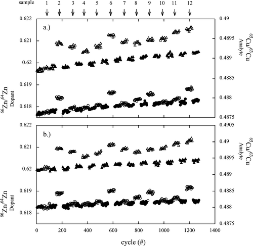

Fig. 1 Copper isotope ratios (analyte, shown as triangles in upper sections of plots (a) and (b) and Zn isotope ratios (dopant, circles in lower sections of plots a and b) of samples (open symbols) and bracketing standards (closed symbols) measured in a SSB session consisting of twelve samples. Plot (a) shows run A and plot (b) shows run B (i.e., the replicate). Sample 1 is an industrial single element standard (Romil Cu) and samples 2 to 12 are granite leachates.

Table 2 δ ⁶⁵Cu values (relative to IMP Cu) of replicate analysis (run A and run B) of one industrial standard and 11 granite leachates, calculated using the various mass bias correction methods discussed in the text. The difference between two methods was calculated using Δ⁶⁵Cu_m-SSB–x = δ⁶⁵Cu_m-SSB – δ⁶⁵Cu_x, where x is d-SSB, EEN or en-SSB. Also shown are the calculated fractionation factors (f_Cu and f_Zn)

Sample type		f Zn	f Cu	δ ^65Cud-SSB	δ ^66Zn	δ ^65Cum-SSB	δ ^65Cuen-SSB	δ ^65CuEEN	Δ^65Cum-SSB – dSSB	Δ^65Cum-SSB – enSSB	Δ^65Cum-SSB – EEN
Run A
1	Industrial standard (Romil Cu)	2.404	2.304	0.021	0.012	0.009	0.008	0.066	–0.01	0.00	–0.06
2	Granite leachate A 96 h1	2.438	2.336	1.258	0.975	0.282	0.192	0.275	–0.98	0.09	0.01
3	Granite leachate G 168 h	2.414	2.312	1.002	0.152	0.850	0.836	0.900	–0.15	0.01	–0.05
4	Granite leachate A 1 h	2.415	2.314	0.645	0.114	0.531	0.521	0.577	–0.11	0.01	–0.05
5	Granite leachate A 48 h	2.421	2.320	0.828	0.195	0.633	0.615	0.648	–0.20	0.02	–0.01
6	Granite leachate H 96 h	2.450	2.348	1.286	0.999	0.287	0.194	0.268	–1.00	0.09	0.02
7	Granite leachate A 2 h	2.424	2.322	0.939	0.129	0.810	0.798	0.843	–0.13	0.01	–0.03
8	Granite leachate A 168 h	2.435	2.333	0.771	0.413	0.358	0.320	0.382	–0.41	0.04	–0.02
9	Granite leachate H 168 h	2.447	2.345	0.840	0.721	0.118	0.052	0.130	–0.72	0.07	–0.01
10	Granite leachate A 10 h	2.428	2.326	0.868	0.074	0.793	0.786	0.833	–0.07	0.01	–0.04
11	Granite leachate B 168 h	2.436	2.334	1.154	0.263	0.891	0.866	0.906	–0.26	0.02	–0.01
12	Granite leachate A 96 h 2	2.460	2.357	1.265	0.926	0.339	0.253	0.289	–0.93	0.09	0.05
Run B
1	Industrial standard (Romil Cu)	2.432	2.330	0.112	0.011	0.101	0.100	0.095	–0.01	0.00	0.01
2	Granite leachate A 96 h 1	2.464	2.361	1.278	0.968	0.310	0.221	0.257	–0.97	0.09	0.05
3	Granite leachate G 168 h	2.439	2.337	0.998	0.154	0.844	0.829	0.872	–0.15	0.01	–0.03
4	Granite leachate A 1 h	2.439	2.336	0.625	0.083	0.541	0.534	0.592	–0.08	0.01	–0.05
5	Granite leachate A 48 h	2.444	2.342	0.793	0.206	0.587	0.568	0.626	–0.21	0.02	–0.04
6	Granite leachate H 96 h	2.471	2.367	1.233	0.982	0.252	0.161	0.256	–0.98	0.09	0.00
7	Granite leachate A 2 h	2.445	2.343	0.943	0.147	0.795	0.782	0.833	–0.15	0.01	–0.04
8	Granite leachate A 168 h	2.454	2.351	0.704	0.378	0.326	0.291	0.346	–0.38	0.03	–0.02
9	Granite leachate H 168 h	2.466	2.363	0.845	0.718	0.127	0.061	0.128	–0.72	0.07	0.00
10	Granite leachate A 10 h	2.447	2.345	0.891	0.103	0.788	0.779	0.825	–0.10	0.01	–0.04
11	Granite leachate B 168 h	2.446	2.343	1.133	0.024	1.109	1.107	1.182	–0.02	0.00	–0.07
12	Granite leachate A 96 h 2	2.478	2.374	1.225	0.984	0.242	0.151	0.269	–0.98	0.09	–0.03

---

3.2. Modified sample–standard bracketing: accuracy of mass bias correction and precision

Fig. 2 shows Cu and Zn isotope ratios in ln–ln space, measured in the bracketing standard solutions during Cu isotope measurements of granite leachates (same samples in Fig. 2(b) and Fig. 1) and Zn isotope measurements of plant samples (Fig. 2(a)). Two important observations are made: first, the spread of ln(⁶⁶Zn/⁶⁴Zn) and ln(⁶⁵Cu/⁶³Cu) is sufficient to achieve a good linear correlation, and second, the relationship of f_Cu/f_Zn (eqn (3)) is constant during each analytical session though significantly different between the analytical sessions and from the theoretical slope of 0.9840 for the exponential law.

Fig. 2 ln(⁶⁵Cu/⁶³Cu) versus ln(⁶⁶Zn/⁶⁴Zn) for doped standards measured during δ⁶⁶Zn determinations of plant digests (plot (a)) and δ⁶⁵Cu determinations of granite leachates (plot (b)). The mass bias relationship f_Cu/f_Zn is determined using a least-squares regression of each data set.

Table 2 shows the calculated mass bias factors f_Cu and f_Zn, δ⁶⁶Zn relative to IMP Zn, and δ⁶⁵Cu of leachates relative to IMP Cu, calculated using the various mass bias correction approaches. Also calculated is the difference between the sample δ⁶⁵Cu ratios derived from the different mass bias correction approaches, using Δ⁶⁵Cu_{m-SSB –x} = δ⁶⁵Cu_{m-SSB – x} – δ⁶⁵Cu_x, where x is d-SSB, EEN or en-SSB. δ⁶⁵Cu values calculated using the m-SSB, en-SSB and EEN approaches are identical within the long-term precision of ±0.1‰. Any inaccuracies associated with the assumptions made using the m-SSB (i.e., f_Cu ≈ f_Zn), EEN (i.e., (f_Cu/f_Zn)_standards ≈ (f_Cu/f_Zn)_samples) and en-SSB (that the exponential law is applicable) are insignificant relative to the levels of reproducibility attained with present day MC-ICP-MS instruments. This observation is also true of δ⁶⁶Zn values measured in plant samples (Table 3).

Table 3 δ ⁶⁵Cu values (relative to IMP Cu) of granite leachates and δ⁶⁶Zn (relative to IMP Zn) of plants using the various mass bias correction methods discussed in the text. The 2σ precision was calculated from two replicate measurements (run A and B)

Sample	Type	δ ^65Cud-SSB	±2σ	δ ^65Cum-SSB	±2σ	δ ^65Cuen-SSB	±2σ	δ ^65CuEEN	±2σ
Granite acid leachates
1	Industrial standard (Romil Cu)	0.07	0.13	0.05	0.13	0.06	0.13	0.08	0.04
2	Granite leachate A 96 h 1	1.27	0.03	0.21	0.04	0.32	0.04	0.27	0.03
3	Granite leachate G 168 h	1.00	0.01	0.83	0.01	0.85	0.01	0.89	0.04
4	Granite leachate A 1 h	0.63	0.03	0.53	0.02	0.54	0.01	0.58	0.02
5	Granite leachate A 48 h	0.81	0.05	0.59	0.06	0.62	0.06	0.64	0.03
6	Granite leachate H 96 h	1.26	0.07	0.18	0.05	0.30	0.05	0.26	0.02
7	Granite leachate A 2 h	0.94	0.00	0.79	0.02	0.81	0.02	0.84	0.01
8	Granite leachate A 168 h	0.74	0.09	0.31	0.04	0.35	0.05	0.36	0.05
9	Granite leachate H 168 h	0.84	0.01	0.06	0.01	0.14	0.01	0.13	0.00
10	Granite leachate A 10 h	0.88	0.03	0.78	0.01	0.79	0.01	0.83	0.01
11	Granite leachate B 168 h	1.14	0.03	0.99	0.33	1.00	0.30	1.04	0.38
12	Granite leachate A 96 h 2	1.24	0.06	0.20	0.14	0.32	0.14	0.28	0.03
Average			0.05		0.07		0.07		0.06
Plant samples (δ^66Zn)
1	Peach leaves GBW 08501	1.23	0.08	0.91	0.03	0.93	0.06	0.91	0.06
8	Peach leaves GBW 08501	1.18	0.23	1.08	0.10	1.07	0.12	1.05	0.13
3	Peach leaves GBW 08501	1.32	0.15	1.46	0.09	1.47	0.10	1.43	0.05
5	Peach leaves GBW 08501	1.26	0.2	1.29	0.12	1.27	0.10	1.22	0.11
2	Ryegrass BCR 281	0.90	0.17	0.74	0.05	0.73	0.05	0.68	0.10
10	Ryegrass BCR 281	1.09	0.19	0.83	0.18	0.82	0.18	0.81	0.10
11	Ryegrass BCR 281	0.90	0.08	0.69	0.10	0.68	0.09	0.65	0.13
4	In-house HRM-14	1.14	0.16	0.80	0.21	0.77	0.23	0.73	0.24
6	In-house HRM-14	0.85	0.27	0.74	0.23	0.71	0.25	0.65	0.18
7	In-house HRM-14	0.88	0.18	0.64	0.08	0.64	0.09	0.60	0.05
9	In-house HRM-14	0.95	0.02	0.84	0.17	0.84	0.17	0.83	0.10
Average			0.16		0.12		0.13		0.11

---

Table 3 shows the calculated ±2σ from replicate analyses (i.e., runs A and B) of sample aliquots during δ⁶⁵Cu and δ⁶⁶Zn determinations of granite leachates and plants, respectively. For the leachates, mean precision is ±0.07‰ or better with all correction methods. For plant samples, the mean precision improves slightly for the δ⁶⁶Zn using m-SSB, en-SSB and EEN compared to d-SSB: however, it is poorer than for the leachates. This likely reflects the complex plant matrix affecting anion-exchange separation procedures and mass spectrometry.²¹ The variation of δ⁶⁶Zn between the four GBW and the four in-house plant samples likely reflects natural fractionation within the plant and the quality of milling and homogenisation of the original sample material. Precisions achieved are in line with reports from other laboratories and/or different instruments^3,4,12,14 and the error is at least 20 times less than natural variability.²²

The mass fractionation coefficients measured on the IsoProbe (2.34 ± 0.02 for f_Cu and 2.44 ± 0.02 for f_Zn) are similar to those measured on another MC-ICP-MS instrument, the Plasma 54 (2.1 ± 0.1).³ We also find that f_Zn is systematically and significantly higher than f_Cu (i.e., f_Cu ≠ f_Zn).

3.3. Generation of variable mass bias for the f_Cu/f_Zn calibration: identifying the best spike element

Fig. 3 shows the effect of spiking the Cu/Zn calibration standards with Sr, Pb or U. When spiked with Sr the range of ln(⁶⁵Cu/⁶³Cu) values is approximately doubled from the typical range obtained with ‘pure’ standards. The range of ln(⁶⁶Zn/⁶⁴Zn) values increased approximately five-fold. However, in contrast to previous observations,¹⁴ Sr-spiked measurements do not form a correlated linear trend and the relationship between the mass bias factors for Cu and Zn breaks down (R² = 0.135). This might be explained by the difference in instrumental settings.²³ Calibration standards spiked with U or Pb form well-correlated linear arrays, with R² = 0.989 and 0.993, respectively. The range of mass bias increases by approximately 25-fold for ln(⁶⁵Cu/⁶³Cu) and 12-fold for ln(⁶⁶Zn/⁶⁴Zn), for both U and Pb. The effects of the Pb spike on the mass bias of the calibration standard series were confirmed with other industrial single element Cu and Zn standards (data not shown).

Fig. 3 ln(⁶⁵Cu/⁶³Cu) versus ln(⁶⁶Zn/⁶⁴Zn) for two series of six IMP Cu/Zn standards (2 µg ml^–1) spiked with Sr (closed circles), U (open circles) and Pb (open diamonds) at a range of concentrations from 0 to 60 µg ml^–1. With the Sr-spike, the spread of data points is increased with respect to pure standards but does not produce a correlated linear trend. Uranium and Pb increase the spread of data further and form a linear relationship.

Fig. 4 shows the effect of matrix concentration on the extent of mass bias variation, expressed in per mil (‰), relative to the unspiked standards. The Pb spike causes the largest deviation for both Cu and Zn, with increases of up to ∼8‰ for δ⁶⁵Cu and ∼9‰ for δ⁶⁶Zn at Pb concentrations of 60 µg ml^–1. The U spike causes an increase of 4–5‰ at 60 µg ml^–1, whereas the Sr matrix effect appears to be comparatively small at ∼1‰.

Fig. 4 Effect of concentration of Sr (closed circles), Pb (open diamonds) and U (open circles) spikes in IMP Cu/Zn standards (2 µg ml^–1) on measured ⁶⁵Cu/⁶³Cu (plot (a)) and ⁶⁶Zn/⁶⁴Zn (plot (b)) expressed as per mil relative to the unspiked standards.

We note a trend between ionisation energy of the spike element and induced mass bias per spike concentration (gradient of the linear regression in Figs. 4 (a) and (b)), given the first ionisation energies of Pb (715.5 kJ mol^–1), U (584 kJ mol^–1) and Sr (549.5 kJ mol^–1). This suggests that the dominant mass bias effect is caused in the plasma rather than in the ion beam, as space-charge effects would result in the heaviest element, U, causing the strongest effect on mass bias.

3.4. Generation of variable mass bias for the f_Cu/f_Zn calibration: using Pb to define the f_Cu/f_Zn relationship during an analytical session

Fig. 5 shows ln(⁶⁵Cu/⁶³Cu) versus ln(⁶⁶Zn/⁶⁴Zn) of the three series of standards Pb-spiked at concentrations between 1 and 40 µg ml^–1. The correlation factor of R² = 0.991 for the combined data set is similar to that for standards without any spike element (Fig. 2). Thus, spiking doped standards with Pb at a range of concentrations significantly increases the variation of mass bias (spread of 13‰ for ⁶⁵Cu/⁶³Cu and 11‰ for ⁶⁶Zn/⁶⁴Zn between highest and lowest ratios) whilst achieving similar correlations. These findings are in line with previous work on the Cu–Zn isotope system conducted by Archer and Vance.¹⁴ Consequently, bracketing an analytical session with series of Pb-spiked standards will allow definition of a dopant/analyte relationship even if the instrumental mass bias is stable.

Fig. 5 ln(⁶⁵Cu/⁶³Cu) versus ln(⁶⁶Zn/⁶⁴Zn) for three series of six IMP Cu/Zn (2 µg ml^–1) calibration standards spiked with Pb matrix at 1–40 µg ml^–1 measured during an analytical session (∼10 hours). The spread of mass bias is significantly greater than for pure standards, covering a range of 11‰ for Cu and 13‰ for Zn between the highest and lowest points. The data set is a combination of all three series measured during an analytical session.

4. Conclusions

Independent mass bias correction schemes applied to a single sample–standard bracketing analytical session assure the accuracy of isotope ratio measurements and act as a solid quality control. This cross-checking of mass bias corrected isotope ratios has been successfully applied to δ⁶⁵Cu and δ⁶⁶Zn determinations in plant and geological samples. The δ⁶⁶Zn and δ⁶⁵Cu values obtained using the m-SSB method agree with values obtained using the EEN and en-SSB methods well within the long-term reproducibility achieved on the IsoProbe MC-ICP-MS. Bracketing the SSB analytical session with a series of calibration standards with varying concentrations of Pb-spike leads to increased variability of mass bias effect, which in turn allows the f_Cu/f_Zn relationship to be defined even when the instrumental mass bias is very stable. This allows the application of the EEN or en-SSB methods and consequently the same solid quality control can be achieved.

Acknowledgements

This work was funded by a Natural Environment Research Council PhD studentship to Kate Peel (NER/S/A/2004/12141), Imperial College London and The Natural History Museum. The authors are grateful to the staff involved in the running and maintenance of the IC/NHM Joint Analytical Facility IsoProbe and, in particular, to the Isotope Geochemistry Group with Mark Rehkämper, Maria Schönbächler, Richard Baker, Simone Gioia, Andrew Berry and Jamie Wilkinson. We also acknowledge three excellent reviews and the editorial help.

References

1. F. Albarède, in Geochemistry of non traditional stable isotopes: Reviews in Mineralogy, eds. C. M. Johnson, B. L. Beard and F. Albarède, Mineralogical Society of America, 2004, vol. 55, pp. 409–427.
2. C. P. Ingle, B. L. Sharp, M. S. A. Horstwood, R. R. Parrish and D. J. Lewis, J. Anal. At. Spectrom., 2003, 18, 219–229.
3. C. N. Maréchal, P. Télouk and F. Albarède, Chem. Geol., 1999, 156, 251–273.
4. T. F. D. Mason, D. J. Weiss, M. Horstwood, R. R. Parrish, S. S. Russell, E. Mullane and B. J. Coles, J. Anal. At. Spectrom., 2004, 19, 218–226.
5. K. G. Heumann, S. M. Gallus, G. Radlinger and J. Vogl, J. Anal. At. Spectrom., 1998, 13, 1001–1008.
6. G. R. Gillson, D. J. Douglas, J. E. Fulford, K. W. Halligan and S. D. Tanner, Anal. Chem., 1988, 60, 1472–1474.
7. D. C. Baxter, I. Rodushkin, E. Engström and D. Malinovsky, J. Anal. At. Spectrom., 2006, 21, 427–430.
8. J. Bermin, D. Vance, C. Archer and P. J. Statham, Chem. Geol., 2006, 226, 280–297.
9. X. K. Zhu, R. K. O’Nions, Y. Guo, N. S. Belshaw and D. Rickard, Chem. Geol., 2000, 163, 139–149.
10. T. Ohno, A. Shinohhara, M. Chiba and T. Hirata, Anal. Sci., 2005, 21, 425–427.
11. A. Stenberg, H. Andrén, S. Malinovsky, E. Engström, I. Rodushkin and D. C. Baxter, Anal. Chem., 2004, 76, 3971–3978.
12. S. Ehrlich, I. Butler, L. Halicz, D. Rickard, A. Oldroyd and A. Matthews, Chem. Geol., 2004, 209, 259–269.
13. M. Rehkämper and K. Mezger, J. Anal. At. Spectrom., 2000, 15, 1451–1460.
14. C. Archer and D. Vance, J. Anal. At. Spectrom., 2004, 19, 656–665.
15. J. D. Woodhead, J. Anal. At. Spectrom., 2002, 17, 1381–1385.
16. A. S. Al-Ammar and R. M. Barnes, J. Anal. At. Spectrom., 2001, 16, 327–332.
17. T. F. D. Mason, D. J. Weiss, M. Horstwood, R. R. Parrish, S. S. Russell, E. Mullane and B. J. Coles, J. Anal. At. Spectrom., 2004, 19, 209–217.
18. J. Chapman, T. F. D. Mason, D. J. Weiss, B. J. Coles and J. J. Wilkinson, Geostand. Geoanal. Res., 2006, 30, 5–16.
19. W. R. Shields, S. S. Goldich, E. L. Garner and T. J. Murphy, J. Geophys. Res., 1965, 70, 479–491.
20. M. Tanimizu, Y. Asada and T. Hirata, Anal. Chem., 2002, 74, 5814–5819.
21. R. Schoenberg and F. von Blankenburg, Int. J. Mass Spectrom., 2005, 242, 257–272.
22. C. Cloquet, J. Carignan and G. Libourel, Environ. Sci. Technol., 2006, 40, 6552–6600.
23. H. Andrén, I. Rodushkin, A. Stenberg, S. Malinovsky and D. C. Baxter, J. Anal. At. Spectrom., 2004, 19, 1217–1224.

---