Modelling and mapping of copper runoff for Europe

Abstract

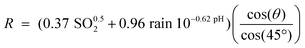
A predictive runoff rate model for copper has been refined and used to generate copper runoff maps for Europe. The new model is based on laboratory and field runoff data and expresses the runoff rate R (g m⁻² yr⁻¹) through two contributions, both with a physical meaning:

Input parameters are the SO₂ concentration (μg m⁻³), pH, amount of rain (mm yr⁻¹), and surface angle of inclination (θ). The first contribution originates from dry periods between rain events (the first-flush effect) and the second from the rain events. The dry term has been refined in comparison to the original model by assuming a mass balance between measured corrosion mass loss, calculated copper retention in the patina and predicted copper runoff. The refined model predicts 76% of all reported runoff rates, worldwide, within 35% from their measured value. This includes sites with low SO₂ concentration, where the original model erroneously predicted higher runoff rates than corrosion rates. Based on environmental data from the EMEP programme for the years 1980–2000, the new model has been used to derive runoff rate maps for Europe with 50 × 50 km grid resolution. The runoff mapping shows a substantial reduction in runoff rate over the investigated time period, and with copper runoff rates now generally less than 2 g m⁻² yr⁻¹.

---

1. Introduction

Due to its favourable properties, such as good corrosion resistance and architectural beauty, copper is widely used in various external constructions such as roofs, facades, claddings, gutters and down-pipes. In recent decades, the concern for possible corrosion-induced metal release (runoff) from external constructions and its environmental effects has gradually increased, and as a result, several legislative actions and restrictions have been implemented towards the use of certain metals, including copper.^1,2 Due to lack of data, the bans are often based on the precautionary principle and conservative deliberations. Extensive research investigations have been implemented during the last decade to fill gaps of knowledge related to the copper runoff process from external structures and its environmental interaction.^3–8 An improved understanding of the corrosion-induced runoff rate mechanism, adequate data, and the availability of a reliable tool for copper runoff rate predictions, are essential to address and estimate copper flows induced by atmospheric corrosion from external constructions in an area. The possibility to predict runoff rates at specific sites, and to identify areas of elevated runoff rates in maps, is essential when assessing corrosion-induced flows of copper in an area. However, it should be noted that potential environmental risks and effects cannot be addressed without taking into account the bioavailability and chemical speciation of released copper.

Dose–response relations based on re-calculations from corrosion rate data exist in the literature for runoff rate predictions.^9,10 More recently, a predictive runoff rate model for copper was developed based on real runoff rate data.¹¹ The model, eqn (1), is derived from extensive information from field studies and detailed laboratory investigations on individual effects of environmental parameters, including rain acidity, intensity and amount as well as corrosion products and composition, surface inclination and orientation.^12,13 Main parameters of the model are rain pH, annual rain quantity and the degree of inclination from the horizontal, all physically explainable parameters known to influence the copper runoff process. A detailed description of the model elaboration is given in ref. 11.

The equation comprises two terms, representing a first flush constant and steady state runoff determined by the rain acidity and the annual rain quantity. The advantage of the model is the fact that all parameters have a physical meaning and that the model is derived from real runoff rate data, as already emphasized above. The disadvantage of the model is that the first flush effect is described by a constant and not by any environmental parameter. As a result, the predictability is less in environments of very high and very low pollutant levels. Due to insufficient data elucidating the effect of corrosive stimulators such as SO₂ on the runoff rate, the constant was not possible to refine when the model was developed.

Corrosion rate maps, based on dose–response functions, have previously been used to identify areas with elevated risk for corrosion, and to select materials to be used in a particular area.¹⁴ However, no maps exist on runoff rates of copper on a European perspective. The only map available is generated for Switzerland and is based on a dose–response relation derived from corrosion rates rather than runoff rates.¹⁵Eqn (1) has recently been used to estimate copper runoff rates for United States.¹⁶

The aim of this paper is to refine the predictive runoff rate model based on pH and annual precipitation quantity, by including the effect of gaseous SO₂, a parameter known to influence the runoff rate of copper.¹¹ In the absence of measured runoff data elucidating the effect of SO₂ on the first flush term, calculated runoff data based on a mass balance are used to refine the model. This is accomplished by applying a statistical analysis of a large set of corrosion and environmental data, including compositional information on patina constituents, collected within an extensive field exposure programme from which runoff rates are calculated. Based on the refined predictive model, maps with a grid size of 50 × 50 km² are presented for corrosion-induced copper runoff rates on a European perspective. The general approach for using mass balance data to refine the predictive runoff rate model, and finally generate runoff rate maps is schematically described in Fig. 1. The figure constitutes the strategy of the paper.

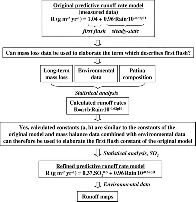Fig. 1 Strategy for using mass balance data to refine the predictive runoff rate model used to generate corrosion-induced runoff rate maps for Europe (a surface inclination of 45° has been used as an example).

2. Experimental

2.1. Compilation of data for mapping

In order to calculate runoff maps, annual average values of environmental parameters included in the runoff model have to be gathered over the region of interest. Table 1 shows a list of the compiled parameters including their unit and abbreviation. Calculation of runoff requires acidity and annual amount of rain as well as SO₂ concentration, while temperature, relative humidity and O₃ concentration are only needed for calculation of the corrosion attack, which in this paper have been used for validation purposes. The co-operative programme for monitoring and evaluation of the long-range transmission of air pollutants in Europe (EMEP) has provided all data on their 50 km × 50 km grid, with the exception of pH. Further information on the EMEP programme can be found at http://www.emep.int.

Table 1 Definition of units for environmental parameters used in the models

Parameter	Unit	Abbreviation
Acidity of rain	Decades	pH
Annual rain quantity	mm yr^−1	Rain
SO2 concentration	μg m^−3	SO2
O3 concentration	μg m^−3	O3
Temperature	°C	T
Relative humidity	%	Rh

---

2.1.1. Acidity of rain (pH). Initiatives like EMEP for modelling transport and wet deposition characteristics do not include acidity of rain as a model parameter. In the future, when particles, basic as well as acidic, are fully included in the models this may be the case but at present stage, the only way to map pH is to gather station data, which are then interpolated.

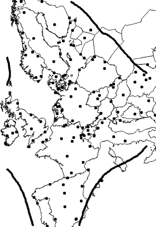
pH data were obtained from EMEP and compiled as annual average data for the period 1980–2000. In order to fill gaps of the partly incomplete data set, and to reduce the measurement error, trend lines were calculated and consequently some outliers removed as described in ref. 14. The predicted values of the trend lines were compiled into complete data sets for the years 1980, 1990 and 2000 for all available stations. Fig. 2 shows the location of these stations on a European map presented in the EMEP projection, which is an equal-area projection. The EMEP projection was selected since all other data are given in this format.

Fig. 2 Map of Europe showing EMEP stations with pH data and calculated interpolation isolines for pH error equal to 0.05 pH units.

The station data was interpolated with the Kriging technique since this enables the estimation of interpolation errors. This error estimate has been used to define the domain of the mapped area allowing only interpolation errors lower than 0.05 pH units (Fig. 2).

All Kriging interpolations have been performed with the Map Info/Vertical Mapper software (http://www.mapinfo.se). A Kriged estimate is a weighted linear combination of known sample values around the point to be estimated. Kriging allows the user to derive weights by means of a so-called semivariogram, which results in optimal and unbiased estimates to avoid over- or underestimates. All interpolations were made with the same semivariogram using a Gaussian model (coincident point distance = 150 km; cell size = 50 km; range = 1200 km; sill = 0.3 pH units; nugget = 0.01 pH units). The sill is the value where the variogram levels off at a certain range. Beyond this range the variable shows no spatial correlation. The nugget is the error that occur over distances much shorter than the sample spacing, and that consequently cannot be resolved. A discussion of the interpolation errors, parameters and their interpretation is given in ref. 17.

2.2. Compilation of literature data on copper runoff rates

Table 2 summarizes available data on measured runoff rates of copper from naturally patinated copper sheet used to illustrate the predictability of the refined predictive runoff rate model (Section 3.4). Due to insufficient environmental data, estimates are in some cases made for the SO₂ concentration. Observed runoff rates at sites 1–20 were included within the generation of the original runoff rate model.¹¹ Newly published independent runoff rates for sites 21–28 have been included to validate the refined runoff rate model.

Table 2 Compilation of available literature data on annual runoff rates of copper from naturally patinated copper sheet

No.	Site (ref.)	Rain/mm yr^−1	pH	SO2/μg m^−3^a	Observed runoff rate/g m^−2 yr^−1	Exp. period/yr
a * Estimated value. b Green patina. c Data not available. d 130 year naturally patinated copper.
1	Washington, DC, USA (18)	958	4.2	27	3.3	3
2	Albany, OR, USA (18)	1084	5.8	0.5*	1.7	3
3	Newport, OR, USA (18)	1822	6.1	0.5*	1.7	3
4	Singapore, Singapore (19)	3138	4.4	22	5.6	1
5	Singapore, Singapore (19)	3203	4.4	22	8.6^b	1
6	Stockholm, Sweden (19)	508	4.6	3	1.4	4
7	Stockholm, Sweden (19)	491	4.6	3	1.6	4
8	Stockholm, Sweden (19)	506	4.6	3	1.4	4
9	Stockholm, Sweden (5)	410	4.6	3	1.4	2
10	Aspvreten, Sweden (5)	450	4.6	0.3	0.8	2
11	Stockholm, Sweden (19)	488	4.6	3	1.5	3
12	Stockholm, Sweden (5)	399	4.6	3	1.2	4
13	Stockholm, Sweden (5)	434	4.6	3	1.7	4
14	Stockholm, Sweden (5)	396	4.6	3	2.0^bd	4
15	Rouen, France (21)	1301	6.0	24	3.1	0.25
16	Connecticut, USA (22)	1400	4.7	15*	2.0^b	^c
17	Stockholm, Sweden (23)	600	4.8	3	0.8^a	0.75
18	Gothenburg, Sweden (24)	425	3.9	30*	4.8^b	1
19	Gothenburg, Sweden (24)	512	4.0	15*	3.2^b	1
20	Gothenburg, Sweden (24)	518	4.3	7*	2.1	1
21	Dübendorf, Switzerland (25)	1161	5.7	7	1.3	2
22	Lägern, Switzerland (25)	1014	5.9	2.9	0.93	2
23	Härkingen, Switzerland (25)	835	5.9	8.3	1.2	4
24	Bern, Switzerland (25)	1184	5.9	7.5	0.8	2
25	Payerne, Switzerland (25)	1061	6.1	2.5	1.1	2
26	Sion, Switzerland (25)	667	5.9	3.5	0.63	4
27	Cadenazzo, Switzerland (25)	1691	5.9	8.5	1.92	2
28	Davos, Switzerland (25)	1199	5.9	1.3	0.72	2

---

3. Results and discussion

The corrosion-induced runoff process takes place at the interface between the atmosphere and the surface of the patina. On a long-term perspective, the runoff rate is relatively constant as long as prevailing environmental conditions do not change significantly.⁸ However, during individual rain episodes, the runoff rate is time dependent with initially high rates during the first portion of rain that decreases to relatively constant rates during the remaining rain event. The total runoff quantity is the sum of these two contributions. On one hand, the first flush portion with a magnitude that depends on the attack of corrosive pollutants and prevailing environmental conditions, and on the other hand the contribution during steady state conditions, which primarily is attributed to the chemical dissolution of patina constituents.^2,20 Each contribution is described in the predictive runoff rate model including rain pH and annual rainfall quantities.¹¹

In the following, the first flush term is refined by including the effect of SO₂ on the runoff process. This is accomplished by using mass balance data in accordance with Fig. 1.

3.1 Derivation of a refined predictive runoff rate model using mass balance data

Direct runoff rate measurements are costly and time consuming since they require dedicated personnel who constantly monitor and collect rainwater impinging on the surface. Due to the irregular nature of precipitation events and seasonal effects, at least one year of measurements is necessary. By sampling only single rainfall measurements, the results can be very different from an annual perspective.

An alternative method to estimate metal runoff (R) is to use a simple mass balance equation since the total amount of corroded metal (Me_total) is either released to the environment in the runoff water, or remains on the metal surface as corrosion products (Me_retained):

R = Me_total − Me_retained (2)

However, such estimates require detailed monitoring and understanding of the kinetics of the corrosion process on a long-term perspective, at least more than one year, since the corrosion rate is highly time-dependent, as well as detailed knowledge of the formation and evolution of corrosion products within the patina. Eqn (2) enables the use of data sets from long-term corrosion exposure programmes for estimating runoff rates. Such estimates require, however, a test programme that comprises a large number of test sites with data collected by a uniform methodology. Since such exposures and generated data are not targeted to estimate runoff rates, essential data are often partly missing.

3.1.1 Description of data set and calculation of runoff rates derived from corrosion data

The basis for the present analysis is data from the International co-operative programme on effects on materials including historic and cultural monuments, “ICP Materials”.²⁶ Within this programme an extensive exposure was performed in the period 1987–1995 with available data after 1 (1987–1988), 2 (1987–1989), 4 (1987–1991) and 8 (1987–1995) years of exposure. In total 39 exposure sites in 12 European countries and in the United States and Canada were involved. All materials were exposed at 45° from the horizontal, facing south. The environment was extensively characterised at each test site and exposure period.²⁷ However, the present analysis only considered the parameters given in Table 1, ozone excluded. The mass loss (ML), the difference in mass before exposure and after pickling, and weight increase (WI), the difference in mass before and after exposure, were determined after each exposure period for freely exposed copper sheets within the exposure program.²⁸ Thus, the sum of ML and WI is ideally equal to the total mass of corrosion products formed during the specific exposure period. However, gravimetric information is not sufficient for calculating the runoff, which in addition requires compositional information, eqn (3):

R = ML − z(ML + WI) (3)

where z is the relative amount of copper in the corrosion products (weight-based).

Average z values were calculated for all exposure periods and test sites based on compositional analysis from the investigation of patina constituents on freely exposed copper within the extensive field exposure programme.²⁹ Main patina constituents besides Cu₂O (z = 0.89), was Posnjakite or Cu₄SO₄(OH)₆·H₂O (z = 0.54), Brochantite or Cu₄SO₄(OH)₆ (z = 0.56), Strandbergite or Cu_2.5SO₄(OH)₃·2H₂O (z = 0.46), Langite or Cu₄SO₄(OH)₆·2H₂O (z = 0.52), Antlerite or Cu₃SO₄(OH)₄ (z = 0.54), and to a much lesser extent, Nantokite or CuCl (z = 0.64), and Atacamite or Cu₂Cl(OH)₃ (z = 60). It should be noted that all copper samples were exposed as in traditional corrosion exposures, i.e. with both the upper and lower side exposed to the environment. This is in contrast to panels used for direct runoff measurements, where the lower side is usually masked and only the upper side exposed. The relevant quantity is of course the runoff from the upper side and not the average runoff from the upper and lower sides given by eqn (3). It should be safe to assume that the runoff from the back side is lower than the runoff from the upper side. A more realistic scenario is that the runoff from the back side is negligible, and the equation is modified according to:

R/2 = ML − z(ML + WI) (4)

Eqn (4) was used to derive calculated runoff values based on mass balance data.

3.1.2 Statistical analysis

Based on the compiled database of 4 × 39 values of calculated runoff rates (R), SO₂ concentration, annual rain quantity (rain), pH, temperature (T) and relative humidity (Rh), a statistical analysis was performed with the aim of establishing an improved predictive runoff rate model. All equations presented in this section have been estimated using this database and using the following general form for the time (t) dependence:

log{R} = log{F(SO₂, rain, pH)t} (5)

However, the results of all estimations are presented below in the form valid for calculation of 1 year runoff values:

R = F(SO₂, rain, pH) (6)

The logarithmic transformation is made to account for the logarithmic distribution of R and the associated errors. Lognormal distribution is common for corrosion values and the statistical analyses support this assumption for the calculated runoff values.

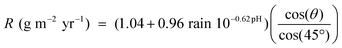
Before estimating models that are more complicated it is worthwhile to derive equations of the same type as eqn (1) based on direct runoff rate measurement in order to validate the database (R = 1.04 + 0.96 rain 10^−0.62pH with an inclination of 45° from the horizontal). Hence, a similar approach to derive the calculated runoff rate was applied with two terms, representing the first flush as a constant and the steady state term with the rain acidity and the annual rain quantity. The coefficient −0.62 was fixed in the derivation procedure in order to allow direct comparison of the two estimated coefficients.

Based on a statistical analysis of the database, the following equation was obtained:

R = 1.26 + 1.14 rain 10^−0.62pH, R² = 0.68 (7)

The coefficients in the two equations (eqn (1) and (7)) are very similar and not statistically different, which is encouraging considering that the derivation of the two equations was substantially different, i.e. measured runoff rates and calculated runoff rates from mass balance and compositional deliberations using a statistical approach. Consequently, an extensive database of calculated runoff rates is useful and further analysis motivated. We have now reached the point in our strategy illustrated in Fig. 1 by the box “Yes, calculated constants (a,b) are similar to the constants of the original model and mass balance data combined with environmental data can therefore be used to elaborate the first flush constant of the original model”.

As previously discussed, a drawback of eqn (1) is that the effect of SO₂ is not included directly. In the further statistical analysis the term 0.96 rain 10^−0.62pH from eqn (1) was taken as given since this term has been extensively validated with real runoff data. If the SO₂ effect is introduced as a linear term, the resulting equation will still include an intercept but if a non-linear SO₂ dependence is assumed (A SO₂^0.5) the intercept will be insignificant and it is possible to exclude it thereby replacing the constant term with a non-linear SO₂ term.

R = A SO₂^0.5 + 0.96 rain 10^{−0.62 pH} (8)

Estimating the constant A by a statistical fit of the data described above results in the final model:

R = 0.37 SO₂^0.5 + 0.96 rain 10^−0.62pH, R² = 0.70 (9)

Since SO₂ is an acidifying pollutant the assumed non-linearity could be physically explained by its relation to the acidity of the aqueous adlayer. For comparison it should be noted that 10^−0.62pH is identical to [H⁺]^0.62. While both terms in the runoff model have a physical meaning, one “dry” term determined by SO₂, and one “wet” term determined by pH, it should be remembered that both parameters are related to each other in a broader perspective.

A statistical analysis of field data using regression analysis has a potential source of error arising from the possible correlations between the involved environmental parameters. In principle, pH may be correlated with SO₂, which also may be correlated to the amount of SO₄²⁻ in precipitation. Table 3 shows a correlation analysis of these parameters, where also SO₂^0.5 and 10^−0.62pH have been included since these are the final explanatory variables included in the model.

Table 3 Correlations between selected environmental parameters and transformed variables from ICP Materials for the exposure periods, 1987–1988, 1987–1989, 1987–1991 and 1987–1995 (150 complete cases)

	pH	10^−0.62pH	SO2	SO2^0.5	SO^2−4
pH	1	−0.92	−0.29	−0.26	0.08
10^−0.62pH	−0.92	1	0.30	0.28	−0.05
SO2	−0.29	0.30	1	0.97	0.62
SO2^0.5	−0.26	0.28	0.97	1	0.58
SO4^2−	0.08	−0.05	0.62	0.58	1

---

The correlation between 10^−0.62pH and SO₂^0.5 is not very high (0.28), which confirms the validity of the function. The reason for the low correlation between pH and SO₂ is due to the local nature of SO₂ pollution, which is more influenced by nearby sources while pH is affected mainly by long distance transport. The network of test sites used for the analysis is a mixure of urban sites with a strong influence of local pollution and rural sites with long distance transport as the main source. Therefore, it is not surprising that the correlation between pH and SO₂ is low. The correlation between SO₂ and SO₄²⁻ is a bit higher (0.62) but still not so high as to disturb the selection of SO₂ over SO₄²⁻. It is not recommended, however, to include both SO₂ and SO₄²⁻ in the same model based on this data set. The correlations between SO₂ and SO₂^0.5 and pH and 10^−0.62pH are very high and therefore selection of one over the other cannot be based on statistical arguments.

As will be shown below, eqn (9) is an improvement over eqn (1) not only from a statistical point of view but it also improves the model predictability, especially when SO₂ is substantially lower than 3 μg m⁻³ or higher than 8 μg m⁻³, where full equality is achieved between eqn (1) and (9).

Unsuccessful attempts were made to improve eqn (9) further by including relative humidity and temperature. This does not mean, however, that these parameters are unimportant for the runoff process.

The angle of surface inclination largely affects the runoff process, showing an expected rain volume dependence determined by the projected area onto which a given rainfall volume impinges.^11–13 Similar to the original predictive model (eqn (1)), the effect of surface inclination needs to be considered in the revised model (eqn (9)):

It should be noted that the model implies no runoff from a vertical façade (θ = 90°). This may not be true at real conditions due to the effect of prevailing wind conditions. However, the effect of wind is not considered in the model. The importance of prevailing wind direction, surface orientation and sheltering has been studied elsewhere.¹³

3.2 Validation of the refined predictive runoff rate model based on comparison with the corrosion attack

The runoff and the corrosion process constitute two quantitative measurements that are governed by different physical and chemical processes. Nevertheless, they are closely linked to each other on a long-term perspective. Even though the instantaneous runoff rate can be higher than the corrosion rate during specific exposure periods due to the release of previously corroded metal, the total amount of runoff can never exceed the total amount of corroded metal. An evaluation of corrosion data from the extensive exposure programme described above has resulted in the following relation for predicting the corrosion attack of copper (inclined 45° from the horizontal) after one year of exposure:²⁶

ML = 0.0027 SO₂^0.32 O₃^0.79Rh e^f(T) + 0.050 rain H⁺ (10)

where f(T) is equal to 0.083(T − 10) when T < 10 °C, otherwise −0.032(T − 10), and H⁺ is the acidity of rain in mg L⁻¹ = 1007.97 10^−pH.

To compare the validation of the refined runoff rate model (eqn (9)) with the original model (eqn (1)), ratios have been calculated between predicted runoff rates and corrosion rates (eqn (10)) for all 50 km × 50 km grid cells. The results (assuming a surface inclination of 45° from the horizontal) are presented in Fig. 3.

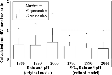Fig. 3 Ratio between runoff and mass loss based on corrosion attack (eqn (10)) and the original (eqn (1)) and the refined predictive runoff rate model (eqn (9)), respectively.

All ratios are typically below 0.5 but the main difference between the models can be observed for the extreme values where the original runoff model with an intercept can predict runoff values exceeding corrosion rates. These over predictions originate from sites typically located in the northern part of Sweden and Norway. It should be noted that in the case of the refined runoff rate model, eqn (9), predicted runoff rates never do exceed corresponding corrosion rates. However, on a short-term perspective, i.e. single rain episodes, the runoff rate can exceed the corrosion rate under certain environmental conditions.³⁰ The model does not consider any potential contribution from background deposition of copper.

3.3 Predictability and validation of the refined runoff rate model based on available runoff rate data

The correlation between observed (Table 2) and predicted runoff rates (surface inclination 45° from the horizontal) is improved for the refined predictive runoff rate model (eqn (9)) compared to the original model (eqn (1)), Fig. 4. Predicted rates versus observed rates exhibit a linear correlation with a regression coefficient increasing from 0.79 to 0.84 and a slope equal to unity, i.e. a 1 : 1 relation intercepting the origin. As a result, the predictability of the refined model is improved compared to the original model, in particular for sites of low SO₂-concentration levels (<3 μg m⁻³). The refined model predicts 76% of all observed rates within 35% from their measured value, Fig. 5. In all, seven out of 29 sites show deviations exceeding ±35% in comparison to observed annual runoff rates. Sites with estimated SO₂ concentrations (sites 2, 3, 16) are included in this group.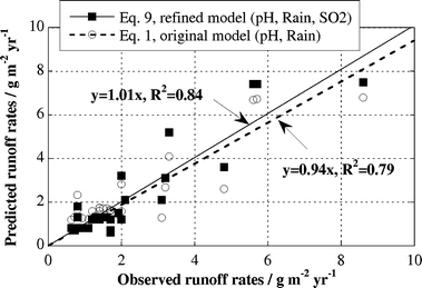

Fig. 4 Relation between observed and predicted annual runoff rates of copper based on the original (eqn (1)) and refined (eqn (9)) runoff rate model.

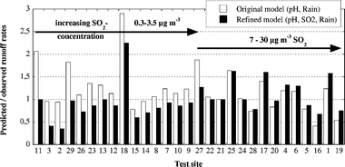Fig. 5 Ratio between observed (Table 2) and predicted annual runoff rates of copper based on the original (eqn (1)) and refined (eqn (9)) runoff rate model. Data are sorted according to the SO₂-concentration at each site.

3.5 Maps of pH, Rain and SO₂ and the generation of maps for copper runoff rates

Changes in rain pH, rainfall quantity and SO₂-concentration are presented as maps on a European perspective in Fig. 6–8 for the years 1980, 1990 and 2000. Corresponding runoff rate maps of copper, based on the refined model (eqn (9)) and a surface inclination of 45° from the horizontal, are displayed in Fig. 9. The trend in SO₂-concentration, rain acidity and runoff rate is obvious with a substantial reduction for the 20 year period illustrated. This reduction is quantified in Table 4 based on an analysis of median values. It should be noted that the reduction in percentage has a general validity also for higher and lower values of environmental data and predicted runoff rates.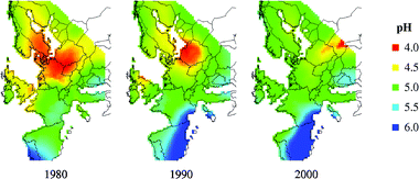

Fig. 6 Acidity of rain (pH) maps for 1980, 1990 and 2000.

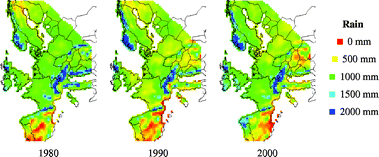Fig. 7 Annual rainfall quantity (Rain) maps for 1980, 1990 and 2000.

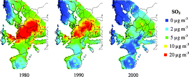Fig. 8 SO₂ concentration maps for 1980, 1990 and 2000.

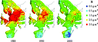Fig. 9 Predicted runoff rate maps of copper, for a surface inclined 45° from the horizontal, for 1980, 1990 and 2000.

Table 4 Median values of rain pH, annual rain quantity (rain), SO₂ and calculated runoff rates, and the relative ratio of 1980 and 2000 values

Parameter	1980	1990	2000	2000/1980
a With rain acidity represented as H^+ = 10^−pH.
pH	4.66	4.90	5.00	46%^a
Rain	865	718	788	91%
SO2	6.0	3.8	1.6	26%
R (eqn 9)	1.99	1.50	1.14	57%

---

The predictive runoff rate map for 2000 shows that there are only some areas with runoff rates of 3 g m⁻² yr⁻¹ copper, i.e. sites with high annual rainfall quantities, low rain pH and or high SO₂-concentration. The general conclusion is that the runoff rates of copper on a European perspective are less than 2 g m⁻² yr⁻¹. It should be noted that the grid size used for presentation, 50 km × 50 km, is relatively large and that substantial variation of the environmental parameters occur within each grid, especially for SO₂ in urban areas. If local maps should be produced, a higher resolution must therefore be used. It should also be noted that the possible effect of chlorides on the runoff process has not been taken into account, which may have a profound effect in coastal areas and in areas affected by de-icing salts distributed on the roads. However, in a recent study of runoff rates of copper in a marine environment for one year, the effect of chlorides was not very significant.³¹

4. Conclusions

The original predictive runoff rate model for copper¹¹ is written as:
in which the first and second terms represent contributions during dry and wet periods, respectively. With more runoff rate data available it has turned out that the model frequently overestimates copper runoff rates at sites with low SO₂ concentration, the reason being the dry (constant) term. A new effort has been undertaken to refine the model. This has been accomplished assuming a mass balance between measured corrosion mass loss from the ICP Materials exposure programme,²⁸ calculated copper retention in the patina based on corrosion product analyses,²⁹ and predicted copper runoff. The refined model is written as:
with SO₂ concentration (μg m⁻³), pH, amount of rain (mm yr⁻¹) and surface inclination (θ) as input parameters. It predicts 76% of all reported runoff rates, in all from 28 sites worldwide, within 35% from their measured value. In particular, the refined model shows a better predictability for the sites with low (<3 μg m⁻³) SO₂ concentration. The model enables the possibility to predict runoff rates at specific sites, and to identify areas of elevated runoff rates in maps. Based on environmental data from the EMEP programme for the years 1980–2000 and from the new model, maps displaying rain pH, annual rain quantity, SO₂ concentrations and predicted copper runoff rates have been constructed for Europe with 50 × 50 km grid resolution. The maps show a clear reduction in rain pH and SO₂ concentration. As a result, runoff mapping shows a substantial reduction in runoff rate over the investigated time period, and with copper runoff rates now generally less than 2 g m⁻² yr⁻¹ for a surface inclined 45° from the horizontal.

Acknowledgements

The authors gratefully acknowledge the financial support from the European Copper Institute, the Swedish Graduate Engineers Association, CF, the United Nations Economic Commission for Europe and the Swedish Environmental Protection Agency. Dr Faller at Swiss Federal Laboratories for Materials Testing and Research (EMPA) is highly appreciated for providing environmental data related to the sites located in Switzerland.

The Co-operative programme for monitoring and evaluation of the long-range transmission of air pollutants in Europe (EMEP) is gratefully acknowledged for providing environmental data.

References

1. International Programme on Chemical Saftety (IPCS), Environmental Health Criteria Document on Zinc, Geneva, Switzerland, November, 1996.
2. Electing multiproblem chemicals for risk reduction—a presentation of the Swedish Sunset Project, KemI, report 13/94, the Swedish National Chemical Inspectorate, Stockholm, Sweden, 1994.
3. I. Odnevall and C. Leygraf, Corros. Sci., 1997, 39(12), 2039.
4. W. He, I. Odnevall Wallinder and C. Leygraf, Corros. Sci., 1998, 40(11), 1977.
5. I. Odnevall Wallinder and C. Leygraf, Corros. Sci., 2001, 43(12), 2379.
6. C. Karlén, I. Odnevall Wallinder, D. Heijerick and C. Leygraf, Environ. Pollut., 2002, 120(3), 691–700.
7. S. Bertling, F. Degryse, I. Odnevall Wallinder, E. Smolders and C. Leygraf, Environ. Toxicol. Chem., 2006, 25(3), 683–691.
8. S. Bertling, I. Odnevall Wallinder, D. Berggren and C. Leygraf, Environ. Toxicol. Chem., 2006, 25(3), 891–898.
9. V. Kucera, J. Tidblad and A. A. Mikhailov, Mapping Air Pollution Effects on Materials Including Stock at Risk, ed. V. Kucera and H.-D. Gregor, bulletin 108E, Swedish Corrosion Institute, Stockholm, Sweden, 2000.
10. A. U. Leuenberger-Minger, M. Faller and P. Richner, Mater. Corros., 2002, 53, 157–164.
11. I. Odnevall Wallinder, S. Bertling, X. Zhang and C. Leygraf, J. Env. Monit., 2004, 6, 704–712.
12. W. He, I. Odnevall Wallinder and C. Leygraf, Corros. Sci., 2000, 43(1), 127.
13. I. Odnevall Wallinder, P. Verbiest, W. He and C. Leygraf, Corros. Sci., 2000, 42(8), 1471.
14. J. Tidblad and V. Kucera, KI-Rapport 2003:4E, Swedish Corrosion Institute, Stockholm, Sweden, 2003.
15. D. Reiss, B. Rihm, C. Thoni and M. Faller, Water, Air, Soil Pollut., 2004, 159, 1–101.
16. R. Arnold, Int. Environ. Assess. Manag., 2005, 1(4), 333–342.
17. M. E. R. Gustavsson, Marine Aerosols in Southern Sweden, thesis, Göteborg University, Göteborg, Sweden, 1999, ISSN 1400–3813.
18. S. D. Cramer, S. A. Matthes, B. S. Covino, S. J. Bullard and G. R. Holcomb, Outdoor and Indoor Atmospheric Corrosion, ASTM STP 1421, ed. H. E. Townsend, American Society for Testing and Materials, West Conshohocken, PA, 2002.
19. I. Odnevall Wallinder, T. Korpinen, R. Sundberg and C. Leygraf, Outdoor and Indoor Atmospheric Corrosion, ASTM STP 1421, ed. H. E. Townsend, American Society for Testing and Materials, West Conshohocken, PA, 2002.
20. C. Karlén, I. Odnevall Wallinder, D. Heijerick and C. Leygraf, Environ. Pollut., 2002, 120, 691.
21. S. Jouen, M. Jean and B. Hannoyer, Surf. Interface Anal., 2000, 30, 145.
22. B. Boulanger and N. P. Nikolaidis, J. Am. Water Res. Assess., 2003 , paper 01149, 1.
23. D. Persson and V. Kucera, Wat. Air, Soil Pollut., Focus, 2001, 1(3–4), 133.
24. V. Kucera and M. Collin, Eurocorr ’77, 6th Int. Congr. Met. Corros., 1977, 189.
25. M. Faller and D. Reiss, Mater. Corros., 2005, 56(4), 244.
26. J. Tidblad, V. Kucera and A. A. Mikhailov, ICP Materials Report No 30, Swedish Corrosion Institute, Stockholm, Sweden, 1998.
27. J. Henriksen, A. Dahlback, K. Arnesen, U. Elvedal and A. Rode, ICP Materials Report No 21, Norwegian Institute for Air Research (NILU), Kjeller, Norway, 1997.
28. B. Stöckle, A. Krätschmer, M. Mach andR. Snethlage, ICP Materials Report No 23, Bavarian State Conservation Office, Münich, Germany, 1998.
29. A. Krätschmer, I. Odnevall Wallinder and C. Leygraf, Corros. Sci., 2002, 44, 425–450.
30. W. He, I. Odnevall Wallinder and C. Leygraf, Water, Air, Soil Pollut., 2001, 1, 67.
31. J. Sandberg, I. Odnevall Wallinder, C. Leygraf and N. Le Bozéc, Corros. Sci., 2006, 48(12), 4316–4338.

---