A small subsurface ion mobility spectrometer sensor for detecting environmental soil-gas contaminants

Abstract

A small subsurface ion mobility spectrometer (SS-IMS) was constructed and tested with several environmental contaminants to determine its potential for monitoring gaseous volatile organic compounds in the vadose zone. Trichloroethylene (TCE) and tetrachloroethylene (PCE) were detected and separated in IMS for the first time. Detection limits as low as 1 part per billion volume-to-volume (ppb_v) were observed. Reduced mobility (K₀) values were reported for 11 environmental contaminants. These data demonstrated the potential of ion mobility spectrometry as a viable technology for detecting and separating environmental soil-gas contaminants in the field, which may lead to a practical and simple approach for long-term monitoring of contaminated soils.

---

Introduction

Human activities have resulted in the contamination of soil to such an extent that the problem is now immense. In the USA alone, the EPA estimated that 1.8 × 10⁹ m³ of ground water and 75 × 10⁶ m³ of soil are contaminated with volatile organic compounds (VOCs).¹ Two contaminants of concern are tricloroethylene (TCE) and tetrachloroethylene (PCE). The Agency for Toxic Substance and Disease Registry (ATSDR) has documented TCE and PCE as the most frequently reported contaminants in ground water. It is estimated that 9 and 34% of drinking water supplies have some TCE and PCE contamination.^2,3 Acute and chronic inhalation exposure to TCE and PCE can affect the human central nervous system, with symptoms such as dizziness, headaches, confusion, euphoria, facial numbness, and weakness. Liver, kidney, immunological, endocrine, and developmental effects have also been reported in humans.²

Existing methods for the detection and measurement of VOCs in the vadose zone (e.g., the volume of soil located between the surface and ground water table, where the spaces between soil particles are filled with both water and air) can be classified according to the method of sample collection. Passive sampling methods involve the burial of a sorbent collector, which adsorbs the VOC from the soil pore gas as a result of diffusion, which is then removed and analyzed.⁴ Results are typically reported as total absorbed mass, as the volume of soil gas has come in contact with the sorbent is unknown.^4,5

Active sampling involves the insertion into the soil of a sampling tube or probe that allows a gas sample to be extracted and brought to the surface for analysis, often using a field gas chromatograph (GC) with flame ionization or electron capture detection (GC-FID or GC-ECD). Alternatively, gaseous samples can be collected in Summa canisters or Tedlar bags and sent to a laboratory and analyzed using a GC with mass spectrometry detection according to EPA SW-846 methods 8260B or 8021, or EPA method TO-15. Active sampling is typically expensive and labor intensive, which generally limits its use to short-term projects such as mapping contaminant plumes.⁵

Headspace sampling followed by GC-mass spectrometry (MS) for detecting VOCs in aqueous samples including TCE and PCE has been described in the literature.⁶ Purge and trap sampling followed by GC-MS analysis have also been described for the analysis of TCE and PCE among other halogenated compounds.⁷ Gas chromatography electron capture detection (GC-ECD) of VOCs in aqueous samples,⁸ halogenated VOCs from surface waters, estuarine, river water and industrial effluents,⁹ organo-halogen compounds in both indoor and outdoor air,^10,11 VOCs in the tropospheric background¹² and halogenated hydrocarbons at trace levels¹³ have been reported.

Other VOCs of environmental significance are methyl tert-butyl ether (MTBE) and methyl iso-butyl ketone (MIBK). MTBE has been widely used as an octane-enhance replacement for lead in gasoline. It causes headaches, dizziness, irritated eyes, coughing, and disorientation and is classified as a human carcinogen. Because of its high solubility in water, a major challenge for analytical chemists is the detection of MTBE in surface and ground waters. In 2004, Pozzi et al.¹⁴ constructed an on-line direct headspace IMS for determining MTBE in water-borne samples, which showed potential for a simple and reproducible technique for rapid MTBE analysis. Baumbach et al.¹⁵ constructed an IMS with both radioactive and UV ionization sources with a multi-capillary column for the determination of MTBE and benzene, toluene, ethylbenzene, and xylene in gaseous and aqueous matrices.

One approach that has shown promise for characterizing contaminated sites in real time is the use of a membrane interface probe (MIP) (Geoprobe Systems, Salina, Kansas) in conjunction with an ion-trap mass spectrometer (ITMS). The MIP is driven into the ground, and gaseous VOCs are collected through a membrane that is permeable to gas but not liquid. Carrier gas move samples to the surface where they are analyzed with the direct sampling ITMS. Results showed a good correlation between samples taken from below the ground water table; however results from vadoze zone tests were influenced by soil type.¹⁶

Another innovative approach to monitoring gaseous contaminants in the environment is ion mobility spectrometry. In 2000, Eiceman et al.¹⁷ described the use of a first-generation radio frequency-based IMS-like drift tube for monitoring VOCs in ambient indoor and outdoor air. This work accomplished three objectives: (1) the continuous measurement of air composition over hours and weeks, (2) the identification of performance features in micro-machined drift tubes and (3) demonstration of the feasibility of this sensor technology for monitoring in the field. In another work, Utriainen et al.¹⁸ combined a metal oxide semiconductor gas sensor with an IMS to produce data with sensitivity and specificity to various chemical vapors in work environments.

Small IMS tubes have been used for explosives monitoring in airports, identifying drugs by customs agents, and chemical warfare agent detection.^17,19 Examples of companies developing small IMS tubes include SANDIA, Oak Ridge National Laboratory, GE Ion Track, Smiths Detection and Bruker Daltonik GmbH.

One of the main advantages of IMS is its ability to provide real-time measurements. This advantage allowed VOCs to be rapidly located and measured, thereby avoiding the distortions of time weighted average responses obtained from passive sampling techniques.²⁰ IMS has intrinsic advantages for on-site monitoring of ambient air including specificity when one considers the principles of ion formation and characterization at ambient pressure. Other examples where IMS instruments have been used for field measurements include industrial stack monitoring,^21,22 vapor drift studies²³ and indoor air quality monitoring.²⁴ In each of these studies the primary focus was that environmental applications with IMS and IMS-like analysis in the field could lead to cost effective analyses. However, IMS has not been developed or investigated for monitoring soil gases.

In this work, the potential for monitoring soil gases by a small SS-IMS, specifically designed to fit inside a 5 cm od cone penetrometer housing was investigated. The IMS, constructed from a machinable glass material called Macor (Corning Inc., New York, USA), was employed for detecting a range of VOCs commonly encountered in the subsurface. Macor was chosen as the construction material for the following advantages: it is easily machinable with ordinary metal-working tools; it can be operated at much higher temperatures compared to other materials like alumina oxide; because of its low thermal conductivity, it is a useful high temperature insulator; it is also an excellent electrical insulator; it has no porosity and, when properly conditioned, will not outgas.

The goal of this research was to evaluate this new sensor for use in obtaining rapid on-site measurements of VOCs. To our knowledge a small IMS sensor for the detection of subsurface gaseous VOCs has not been previously described.

Experimental

Instrumentation

The small SS-IMS used in this investigation was designed and constructed at Boise State University in collaboration with Washington State University, and tested at Washington State University. The instrument was comprised of the following units: (1) 15 MBq ⁶³Ni radioactive foil; (2) reaction region; (3) Bradbury–Nielsen ion gate; (4) counter-flow atmospheric pressure drift region; (5) aperture grid; (6) Faraday plate and (7) data acquisition system. Fig. 1 shows a cross-sectional view of the SS-IMS. Table S1 (ESI†) summarizes the operating conditions and drift gases used in this investigation.

Fig. 1 Cross-sectional schematic view of the subsurface ion mobility spectrometer used in this work.

Both the reaction and drift regions were constructed with machined Macor stacked in an interlocking design²⁵ with metal electrodes and Macor insulators in a coaxial arrangement with terminating end caps for a total overall length of 113 mm. Each Macor ring was machined to an od of 38 mm, and thickness of 5 mm. A counter bore was machined into each face of an insulator to provide a pocket for the mating electrode. The drift region insulating rings had a constant id of 22 mm whereas those of the reaction region varied from 11 mm to 22 mm forming a tapered transition region from the ion source to the ion gate entrance. The drift and reaction regions contained 12 and 5 rings, respectively. To generate a uniform electric field down the tube, the stainless steel guard rings were connected to each other through 1 MΩ high-temperature resistors (Caddock Electronics Inc., ±1%).

Carrier gas flowed into the IMS through the reaction region where the ⁶³Ni radioactive foil was positioned. High-energy electrons emitted from the ⁶³Ni radioactive foil initiated the ionization process through collisions with ambient pressure gas. This process resulted in the formation of both positive and negative low-energy reactant ions. The low-energy reactant ions interacted with neutral sample vapors to produce product ions.

At the interface between the reaction and drift region was an electronic Bradbury–Nielsen gate that opened periodically to admit a finite pulse of ions into the drift tube. This design was constructed using parallel Alloy 46 (California Fine Wire Co., Grove Beach, CA) wires (75 μm in diameter) with a 0.25 mm spacing as described previously.²⁶ The gate was ‘closed’ by applying ±24 V to adjacent wires so that a ∼441 V cm⁻¹ closing field was placed orthogonal to the drift tube of the IMS. As positive or negative ions approach the gate they were collected on the negative and positive wires, thereby preventing them from passing through the gate. When the gates were ‘open’ all gate wires were pulsed to a single voltage appropriate to the gate’s position in the drift electric field.

Under the influence of the applied electric field, ions in the drift region were directed towards a novel Faraday plate collector electrode against a counter-flow of atmospheric pressure drift gas at a fixed flow rate. The ratio of the drift velocity of a given ion to the applied field strength generates the ion’s mobility. An aperture grid, located just in front of the Faraday plate, served to filter out electronic noise generated from opening and closing of the gate and to shield the effect of induced current on the Faraday plate from the gas phase ions as they approached the plate. The ion’s average drift velocity is a function of its size and charge. Ions separate according to their size/charge ratio as they traverse the drift tube.

The electronic components for the SS-IMS system included a high-voltage power supply and software controlled gate drivers constructed at Washington State University. Response of the Faraday detector was processed with a Model 427 current amplifier (Keithley Instruments, Cleveland, OH, USA) whose amplification was 10⁹ V A⁻¹. The resulting signal was sent to a personal computer (operating Labview code developed at WSU) through a SHC68-68-EPM noise rejecting shielded cable (National Instruments, Austin, TX, USA). The resulting text file data was then processed using Igor Pro 5.0.3 (WaveMetrics, Portland, OR, USA). Miniaturized versions of the electrical components have been designed for future field use.

Material and reagents

Eleven environmental soil-gas contaminants obtained from Sigma Aldrich Chemical Company (St Louis, MO) were chosen for studies in both positive and negative ion modes. The environmental soil-gas contaminants consisted of trichloroethylene (TCE), tetrachloroethylene (PCE), methylene chloride (DCM), 1,2-dichloroethane (DCE), 1,2,4-trichlorobenzene (1,2,4-TCB), methyl tert-butyl ether (MTBE), methyl iso-butyl ketone (MIBK), acetone, toluene, p-xylene and ethylbenzene. A common IMS calibration standard, 2,4-lutidine, was used in these studies to insure that the IMS was operating properly.

Samples were introduced into the SS-IMS through an exponential diluter. The exponential dilution approach has been described previously.^27,28 In this investigation, an exponential dilution device was constructed from a 3.9 L stainless steel metal canister with a height and a width of 20 and 18 cm, respectively. The canister had two openings; one was used as the inlet and the other, as the outlet. The inlet was fitted with a 1/4″ stainless steel T-union (Swagelok, Tri-Cities Valve & Fitting Co., Richland, WA, USA). One end of the T-union was connected to the canister, the ‘T’ end was used as the carrier gas inlet, and the third end of the union was sealed with 10 mm Thermogreen™ septa (Supelco, Bellefonte, PA, USA). This created the gas-tight injection inlet. A one-way valve (Swagelok, Tri-Cities Valve & Fitting Co., Richland, WA, USA) at the canister outlet was used to switch the carrier gas exiting the flask into the SS-IMS or to the laboratory exhaust hood. Exponential dilution mixing was initiated by injecting a known amount of analyte into the canister via the injection inlet. Injected analytes then flowed through the one-way valve into the IMS reaction region. The effluent concentration declined exponentially and the concentration at each time step can be predicted.

Concentrations for each of the samples at the start of exponential dilution experiment with a flow rate of 10 mL min⁻¹ were the following: 2,4-lutidine, 17 parts per million volume-to-volume (ppm_v); TCE, 76 ppm_v; PCE, 66 ppm_v; DCM, 106 ppm_v; DCE, 87 ppm_v; MTBE, 34 ppm_v; MIBK, 34 ppm_v; acetone, 83 ppm_v; toluene, 64 ppm_v; p-xylene, 56 ppm_v; and ethylbenzene, 55 ppm_v.

Table 1 lists the molecular weight, density and vapor pressure of compounds investigated and Table S3 shows their structures (ESI†).

Table 1 Reduced mobility values for VOCs in drift gases air and nitrogen

Compound	M/g mol^−1	K 0(Air)^c	K 0(N2)^c
a Monomer ions. b Dimer ions. c K 0 are in cm^2 V^−1 s^−1. d Negative chloride ions. e Ns = not seen at concentration studied.
2,4-Lutidine	107.15	1.95^a 1.50^b
TCE	131.39	1.91^a 1.78^b	1.87^a 1.64^b 2.39^d
PCE	165.83	1.81; 1.64; 1.52; 1.45; 1.36	1.78; 1.63; 1.51; 1.44; 1.34; 2.39^d
DCM	84.93	2.39^d shoulder peak	2.39^d
DCE	98.96	2.39^d shoulder peak	2.39^d
MTBE	98.96	1.93^a 1.64^b	1.86^a 1.60^b
MIBK	100.16	1.78^a 1.48^b	1.77^a 1.48^b
Acetone	58.08	1.94	1.93
Toluene	92.14	Ns^e	Ns^e
p-Xylene	106.17	1.74	1.76
Ethylbenzene	106.17	1.82	1.81

---

Calculations

Based on the frequency of ion-molecule interactions, ions possessing different collision cross-sections separate under the influence of a weak homogenous electric field. The mobility (K) of the ion is a ratio of its velocity (ν_d) to the applied electric field (E). Experimentally the relationship in eqn (1) can be used to determine an ion’s mobility:where L is the length of the drift region (cm), t_d is the drift time of the ion (ms), and V is the gate voltage (volts). The mobility of an ion can be normalized to a reduced mobility value (K₀) to account for drift gas temperature (T) and pressure (P) changes. The resulting K₀ is given by eqn (2) which allows for comparison between different experimental systems:where K₀ is reported in cm² V⁻¹ s⁻¹, T is in K, and P is in Torr. A well established performance acceptance criterion for different IMS systems is that the calculated reduced mobility values for known analytes must agree to within 2–3%.

Experimental IMS resolving power (R_exp) is defined as the drift time (t_d) of the ion divided by the peak width at half height (w_0.5)²⁹ as shown in eqn (3).

Resolution (R) is the degree to which two peaks are resolved. R is the result of the difference in drift times (Δt_d) divided by the average baseline peak width (W_base)³⁰where α is the selectivity factor defined as K₀₁/K₀₂ for peaks associated with compounds 1 and 2.

Concentrations of environmental soil-gas contaminants were calculated as follows. For gas injections, the actual headspace volume injected into the exponential dilution flask was given by:

whereThus, the volume of gas sample injected was calculated as:where R is the universal gas constant, T is the room temperature in K, and P is the pressure in atmospheres. Finally the concentration of the analyte in ppm_v is:When pure liquid standards were injected into the exponential dilution flask, the mass of the analyte was calculated from the density and volume of sample injected. This value was converted to moles of analyte injected by dividing the mass with the molecular weight of the analyte. Eqn (7) and (8) were then used to calculate the concentrations. To ensure evaporation of liquid samples, the exponential dilution flask was allowed to stand for one hour after injection before the carrier flow was introduced through the flask and into the IMS.

The exponential dilution strategy used is given by eqn (9):

where [C]_t was the concentration at any time, t, [C]_ppmv is the concentration of gas or liquid injections, f is the carrier gas flow (10 mL min⁻¹), t is the time and v is the volume of exponential dilution canister (3900 mL).

Detection limits were determined from the spectrum as follows:

R_(t) = S[C_i] + B (10)

where R_(t) is the response (nano-ampere, nA), S is the sensitivity (nA ppm_v⁻¹), [C_i] is the concentration (ppm_v) and B is the background current (nA). But the response of an unknown A (R_(t)A) is R_(t)A − B and from eqn (10), R_(t) − B = S[C_i]. At the detection limit where R_(t)A = 3σ, then,

R_(t)A = S[C_i] = 3σ (11)

Rearranging eqn (11) leads to eqn (12):where [C_i]_D is the minimum detectable concentration, σ is the root mean square noise (i.e., the noise above the background current), S = R_(t)/C_i and C_i is the concentration at which detection limit is determined.

Results and discussion

Mobility measurement

Standard environmental soil-gas contaminants were introduced into the IMS to obtain IMS spectra and determine K₀ values in air and nitrogen drift gases. This investigation used 2,4-lutidine as a calibration standard in the positive ion mode. In the positive ion mode the spectrometer only measures the positive ions produced in the ionization process. Negative ions can also be measured by IMS if the polarity of the drift voltage is reversed from a positive voltage to a negative voltage. The measured K₀ values for its monomer and dimer ions in both air and nitrogen drift gases were reported at 1.95 ± 0.01 and 1.50 ± 0.01 cm² V⁻¹ s⁻¹, respectively. These values are in excellent agreement with those of the monomer (1.95 cm² V⁻¹ s⁻¹) and dimer ions (1.50 cm² V⁻¹ s⁻¹) of 2,4-lutidine reported previously in the literature.^28,31,32 Drift times for the water reactant ion peaks (RIP) in the positive ion mode were 6.43 ± 0.03 and 6.33 ± 0.02 ms for air and nitrogen drift gases, respectively. From these drift times, the calculated K₀ values were 2.08 ± 0.01 and 2.09 ± 0.03 cm² V⁻¹ s⁻¹ in air and nitrogen drift gases, respectively.

The K₀ values for all eleven soil-gas contaminants investigated are listed in Table 1. These K₀ values were calculated based on eqn (2) from drift times obtained when the compounds were introduced into the instrument. Fig. 2 and Fig. S1 (in the ESI†) show example responses observed for soil-gas contaminants detected during this investigation. The K₀ values reported in Table 1 for the monomer and dimer ions of MTBE compared to within 9 and 11% respectively to a study with nitrogen reported in the literature.¹⁵ This study used nitrogen as the drift gas and a temperature of 23 °C. The reported K₀ values were 1.69 and 1.42 cm² V⁻¹ s⁻¹ for the monomer and dimer ions, respectively. However, the drift times and pressure used for calculation of the K₀ values were not reported. Since the K₀ of each ion depends on the drift time and pressure, adequate comparison of our data with the literature value could not be made. Another study with MTBE used air as the drift gas and reported the ionization region temperature as 80 °C.¹⁴ Their K₀ values of 1.85 and 1.50 cm² V⁻¹ s⁻¹ reported for the monomer and dimer ions compared to within 4 and 9%, respectively. This study only reported the temperature as that of the ionization region. Also there was no mention of the drift tube length, pressure or voltage at which the measurements were made. Thus, as with the previous study, independent verification of their values could not be made. With MIBK there has been a study that reports IMS spectra at 27, 50, 80, 110 and 140 °C, respectively.³³ This study looked at temperature effect on an IMS tube and made no mention of K₀ values. Thus our work seemed to be the first to measure K₀ values for MIBK in air and nitrogen. The response for MTBE reported here gave monomer ions at 1.93 ± 0.03 and 1.86 ± 0.02 cm² V⁻¹ s⁻¹ and dimer ions at 1.64 ± 0.02 and 1.60 ± 0.01 cm² V⁻¹ s⁻¹ for air and nitrogen, respectively. For MIBK, its monomer ion occurred at 1.78 ± 0.02 and 1.77 ± 0.02 cm² V⁻¹ s⁻¹, whereas the dimer peaks occurred at 1.48 ± 0.01 and 1.48 ± 0.02 cm² V⁻¹ s⁻¹ for air and nitrogen, respectively.

Fig. 2 Ion mobility spectra for TCE and PCE individual responses in the positive ion mode using air (top) and nitrogen (bottom) as drift and carrier gas. The data show that TCE and PCE can be detected in the positive ion mode with the SS-IMS. TCE showed two peaks and PCE showed five peaks in the IMS spectra. The TCE spectra for the air and nitrogen plots were offset by 0.3 nA. Fig. S1 displays responses for acetone, ethylbenzene, p-xylene, MTBE and MIBK.†

In IMS, chlorinated compounds have been analyzed in the negative ion mode¹⁹ and the process by which the product ions are formed has been well documented to occur by dissociative electron capture¹⁴ with the chloride ion being the product ion detected. In this study, some chlorinated compounds were detected in the positive mode after introduction into the IMS. While DCM or DCE were not seen in the positive ion mode, TCE and PCE were detected in this mode by IMS. Two peaks for TCE and five peaks for PCE were detected in the positive ion mode. K₀ values for TCE occurred at 1.91 ± 0.02 and 1.78 ± 0.01 cm² V⁻¹ s⁻¹ for air drift gas. In nitrogen drift gas, however, the K₀ for TCE occurred at 1.87 ± 0.01 and 1.64 ± 0.02 cm² V⁻¹ s⁻¹, respectively. At lower concentrations of TCE, the peaks at K₀ 1.78 and 1.64 cm² V⁻¹ s⁻¹ for air and nitrogen disappeared which indicated that the two K₀ values observed for TCE were probably monomer and dimer ions. Reduced mobility values for PCE in air were 1.81 ± 0.02, 1.64 ± 0.01, 1.52 ± 0.01, 1.45 ± 0.02, and 1.36 ± 0.02 cm² V⁻¹ s⁻¹. In nitrogen, five peaks were also seen at K₀ 1.78 ± 0.01, 1.63 ± 0.01, 1.51 ± 0.01, 1.44 ± 0.02, and 1.34 ± 0.03 cm² V⁻¹ s⁻¹, respectively.

Interestingly, toluene was not detected at the introduced concentration of 64 ppm_v. Ethylbenzene gave reduced mobility values at 1.82 ± 0.02 and 1.81 ± 0.01 cm² V⁻¹ s⁻¹ in air and nitrogen, whereas p-xylene responded at 1.74 ± 0.03 and 1.76 ± 0.02 cm² V⁻¹ s⁻¹ for air and nitrogen, respectively.

In the negative ion mode, drift times for the oxygen RIP in air and nitrogen were 5.98 ± 0.01 and 6.10 ± 0.02 ms, respectively. These drift times gave calculated K₀ values of 2.23 ± 0.01 and 2.20 ± 0.02 cm² V⁻¹ s⁻¹, respectively. Fig. 3(a) showed that the Cl⁻ ions from both DCM and DCE could not be resolved from the strong background ion (probably from oxygen) in air drift gas. Note the shoulders on the background ions of the Cl⁻ ions for both the DCM and DCE responses. Fig. 3(b) was the result of switching the drift gas to nitrogen. Nitrogen drift gas probably contained some oxygen contamination that gave a tiny background ion. This background ion could not be baseline resolved from the Cl⁻ ions with DCM, DCE, TCE, and PCE. Fig. 3(b) also demonstrated that while the Cl⁻ ions from DCM, DCE, TCE, and PCE could be differentiated from the background ion in nitrogen drift gas, these Cl⁻ ions cannot be resolved from each other. All four compounds gave a K₀ value of 2.39 ± 0.01 cm² V⁻¹ s⁻¹ for the Cl⁻ ion. The reduced mobility of the Cl⁻ ions differs from the literature value by 18%. The literature has previously reported K₀ values with different chlorinated compounds from 2.90–3.14 cm² V⁻¹ s⁻¹ for temperatures between 110–300 °C.^34,35 Thus, it was not surprising that the K₀ value reported in this work differed from that in the literature. One reason for the difference in K₀ values for the Cl⁻ ion may be clustering of ions at room temperature. Fig. 3(a) and (b) demonstrated IMS sensors can be used to identify Cl⁻ ions from chlorinated compounds in negative ion mode operation. However, the SS-IMS could not differentiate Cl⁻ ions from different chlorinated compounds.

Fig. 3 Ion mobility spectra for DCM and DCE in the negative ion mode using air (a) and DCM, DCE, TCE and PCE in the negative ion mode using nitrogen (b) as drift and carrier gas. The data show that the chloride ion from both DCM and DCE could not be separated from the background ion in air. Note the shoulders in the responses of DCM and DCE (a). This was expected as air has oxygen that forms a large background ion in the negative ion mode. In plot (a), DCM and DCE in air were offset by −0.54 and −1.1 nA. In plot (b), DCM, DCE, TCE and PCE were offset by −0.1, −0.19, −0.26, and −0.44 nA, respectively.

Sensitivity, signal-to-noise, dynamic range and detection limits

Signal-to-noise ratios as a function of concentration of TCE, and PCE in both and nitrogen are shown in Fig. 4(a) and (b). Similar profiles were observed for MTBE and MIBK. Note that concentrations above the limit of quantification were not shown in the plots. In these plots, the y-axis represents signal-to-noise responses obtained from the detector whereas the x-axis represents calculated concentrations from eqn (9). Firstly, each figure shows the signal-to-noise response of the compound in air and nitrogen as diamonds and circles, respectively. Secondly, the figures demonstrated the concentration responses and their corresponding signal-to-noise ratios delivered by the sample introduction unit. These figures have been corrected for a sample transfer lag time (i.e., the time taken for the sample to travel from the exponential dilution canister to the IMS). These times were 196, 116, 117 and 126 s for TCE, PCE, MTBE and MIBK, respectively. The sensitivity was determined by measuring the average slope of the line between the limits of quantification and limits of detection in Fig. 4(a) and (b). In air drift gas, sensitivity of TCE, PCE, MTBE and MIBK were 1.88, 2.21, 0.96 and 1.50 signal-to-noise ppm_v⁻¹, respectively. In nitrogen drift gas, sensitivity of TCE, PCE, MTBE and MIBK was reported at 2.75, 1.94, 1.25 and 1.86 signal-to-noise ppm_v⁻¹, respectively.

Fig. 4 Plot of TCE (a) and PCE (b) signal-to-noise ratios vs. calculated concentration in air (diamond) and nitrogen (circles) for the sample introduction unit interfaced to the SS-IMS. Similar profiles were obtained with MTBE and MIBK.

For TCE, signal-to-noise ratios were calculated for the peaks at 7.03 ± 0.01 and 7.13 ± 0.01 ms with K₀ of 1.91 ± 0.02 and 1.87 ± 0.01 cm² V⁻¹ s⁻¹ for air and nitrogen, respectively. The signal-to-noise ratios for PCE were determined for the peaks at 7.45 ± 0.02 and 7.48 ± 0.01 ms with K₀ of 1.81 ± 0.02 and 1.78 ± 0.01 cm² V⁻¹ s⁻¹ in air and nitrogen, respectively. For MTBE and MIBK signal-to-noise ratios for the dimer ions were determined. The maximum concentrations of TCE and PCE started at 76 ppm_v and 66 ppm_v, respectively. For MTBE and MIBK, the maximum concentrations started at 34 ppm_v. The signal-to-noise ratios for the background ion in both air and nitrogen were 33 and 35, respectively. The maximum signal-to-noise ratios for TCE in air and nitrogen were 12.33 and 13.05, respectively. The signal-to-noise ratios for PCE were lower than those of the TCE peaks. The maximum PCE signal-to-noise ratio was 5.96 in air and 6.56 in nitrogen. With respect to MTBE and MIBK, the maximum signal-to-noise ratio in air was 65 for both compounds. In nitrogen, signal-to-noise ratios were 70 and 72 for MTBE and MIBK, respectively. The signal-to-noise ratios for TCE and PCE were just 37 and 19% of the background ion, respectively. The signal-to-noise ratio exceeded that of the background ions for MTBE and MIBK by 49 and 53%, respectively.

Detection limits were calculated based on eqn (12), and the minimum values were reported for acetone, MTBE and 2,4-lutidine at 1 ppb_v whereas the detection limit of 10 ppb_v reported for p-xylene was the largest detection limit observed in this study. The upper limit of quantification was reported for PCE at 10 ppm_v and the maximum at 37 ppm_v for p-xylene. Figs. 4(a) and (b) further demonstrate that the calculated limits of detection and quantification fall within the experimental range. Table 2 lists detection limits and limits of quantification for the other environmental soil-gas contaminants studied. The results demonstrated that the SS-IMS sensor can detect environmental soil-gas contaminants in the ppb_v range.

Table 2 Detection limits and limits of quantification of environmental soil-gas contaminants studied

Compound	Detection limit (ppbv)	Limit of quantification (ppmv)
2,4-Lutidine	1	13
TCE	6	11
PCE	8	10
MTBE	1	17
MIBK	3	13
Acetone	1	15
p-Xylene	10	37

---

SS-IMS resolving power

Experiments were conducted by changing the drift gas flow rate from 100 to 1000 mL min⁻¹ while the carrier gas flow rate was maintained at 10 mL min⁻¹. Resolving powers were calculated for the TCE peak at 7.08 ± 0.01 ms and the PCE peak at 7.43 ± 0.02 ms. Fig. 5(a) and (b) show the result generated from a plot of resolving power vs. drift gas flow rate in air and nitrogen drift gases. In commercial IMS sensors, resolving powers no greater than 30 have been reported³⁰ under standard operating conditions. The spatial spreading of an ion peak arriving at the detector t_d s after being admitted to the drift region is governed by its diffusion coefficient.²⁹ Thus the drift gas flow rate was found to have a minimal effect on resolving power of TCE and PCE as demonstrated in Fig. 5(a) and (b).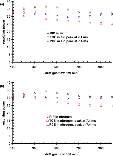

Fig. 5 Plot of reactant ion peak (RIP), TCE and PCE resolving power vs. drift gas flow rate in air (a) and nitrogen (b) drift gases.

In air, the RIP gave a maximum resolving power of 32 at 300 mL min⁻¹ whereas in nitrogen, the maximum resolving power of 31 occurred at 800 mL min⁻¹. Based on the experimental resolving powers measured in this investigation and the expected theoretical resolving power determined with the instrument settings reported in Table S1,† resolving power efficiency of the small SS-IMS drift tube was estimated. The RIP in air gave an efficiency of ∼57% at 300 mL min⁻¹, whereas in nitrogen an efficiency of ∼54% at 800 mL min⁻¹ was obtained.

The maximum resolving power (33, resolving power efficiency of ∼61%) for TCE in air occurred at 100 mL min⁻¹. Fig. 5(a) shows that at 400 mL min⁻¹, the resolving power of TCE decreased rapidly tailing off at 25 (∼38% efficiency) for 1000 mL min⁻¹. In air, the maximum resolving power (37, resolving power efficiency of ∼78%) of PCE occurred at 400 mL min⁻¹ with the drop occurring above 500 mL min⁻¹. A similar profile was noted in nitrogen, Fig. 5(b), with maximum resolving powers of 31 (∼54% efficiency) and 34 (∼64% efficiency) occurring for TCE at 200 mL min⁻¹ and PCE at 400 mL min⁻¹, respectively. This study demonstrated that the SS-IMS used in this investigation behaved similarly in experimental resolving power to already existing commercial IMS sensors used for explosives and drugs detection in the field.³⁰ The data further demonstrated that there is some broadening of peaks for drift gas flow rates above 400 mL min⁻¹. The reason for this behavior is not clear and will require a more detailed and systematic investigations to delineate the mechanisms of clustering and de-clustering of mobility ions at room temperature. Detailed studies are already underway to investigate the combined effect of voltage and gate pulse width on resolving power. The main goal for developing the SS-IMS is to insert it into a cone penetrometer housing for operation in the subsurface with as low of gas flows as possible. Thus, these results are significant for the device under development, as they will facilitate optimization of the device.

SS-IMS resolution

Although TCE and PCE have not previously been separated by IMS, these studies demonstrated that such separation is possible. With commercial IMS systems, a Δt_d value of at least 0.6 ms is needed³⁰ to produce baseline resolution of two peaks. When TCE and PCE were introduced as a mixture to the SS-IMS, resolution was possible. Fig. 6(a) shows an IMS separation of TCE and PCE in air and nitrogen drift gases, respectively. In air, drift times of 7.05 ± 0.01 and 8.18 ± 0.03 ms correspond to drift times and mobilities of TCE measured individually as presented in Fig. 2 and Table 1. Drift times of 7.43 ± 0.01, 8.18 ± 0.01, 8.78 ± 0.02, 9.25 ± 0.01 and 9.93 ± 0.01 ms correspond to drift times and hence mobilities of PCE in air measured individually as presented in Fig. 2 and Table 1. In nitrogen, the respective drift times of 7.13 ± 0.01 and 8.35 ± 0.01 ms were reported and correspond well to drift times and mobilities of TCE measured individually and presented in Fig. 2 and Table 1. The PCE drift times in nitrogen occurred at 7.63 ± 0.01, 8.35 ± 0.02, 9.35 ± 0.01 and 10.05 ± 0.01 ms and they correspond well to drift times and mobilities measured individually and presented in Fig. 2 and Table 1. Note that the peaks at 8.18 ms in air and 8.35 ms in nitrogen were the second peaks for both TCE and PCE. These two peaks could not be separated by the SS-IMS used in this investigation. However, separation of the first peak of both TCE and PCE enabled the two compounds to be differentiated in positive ion mode IMS.

Fig. 6 (a) IMS spectra for TCE and PCE mixtures in air and nitrogen drift gases. The top spectrum was offset by 0.24 nA. 1, 2, 3 and 2 & 3 represent the RIP, TCE, PCE and TCE & PCE, respectively. Note that the peaks labeled 2 & 3 were the first peaks of both TCE and PCE and these peaks were separated by the SS-IMS used in this investigation. (b) IMS spectra for TCE and PCE; DCM, DCE, TCE and PCE; TCE, PCE and chloroform mixtures in air drift gas. The top spectra were offset by 0.24 and 0.48 nA, respectively. 1, 2, 3 and 2 & 3 represent the RIP, TCE, PCE and TCE & PCE, respectively.

DCM, DCE, TCE and PCE were introduced as mixtures to determine whether DCM or DCE would interfere with the responses of TCE or PCE. In addition, chloroform interference on the responses of TCE and PCE was investigated. Fig. 6(b) shows an IMS separation of TCE and PCE, DCM, DCE, TCE and PCE, TCE, PCE and chloroform in air. For DCM, DCE, TCE and PCE mixture, the drift times of 7.13 ± 0.01, 7.58 ± 0.01, 8.33 ± 0.02, 9.33 ± 0.02 and 10.08 ± 0.02 ms correspond well to the mixture of TCE and PCE presented in Fig. 6(a). The drift times of 7.23 ± 0.02, 7.65 ± 0.02, 8.43 ± 0.01, 9.38 ± 0.01 and 10.2 ± 0.01 ms obtained for the drift times of TCE, PCE and chloroform mixture corresponded well to the mixture of TCE and PCE presented in Fig. 6(a). In nitrogen, IMS responses for the same mixtures reported in Fig. 6(b) were as follows. The drift times for the DCM, DCE, TCE and PCE mixture in air were 7.23 ± 0.01, 7.65 ± 0.02, 8.40 ± 0.01, 9.38 ± 0.02 and 10.10 ± 0.01 ms. These responses correspond well to the responses from the mixture of TCE and PCE presented in Fig. 6(a). The drift times for the TCE, PCE and chloroform mixture in air were 7.23 ± 0.01, 7.73 ± 0.03, 8.43 ± 0.03, 9.48 ± 0.01 and 10.15 ± 0.02 ms and they correspond to the responses of TCE and PCE mixture presented in Fig. 6(a). The fact that the responses obtained correspond to the responses of TCE and PCE measured individually and in a mixture, demonstrated DCM, DCE and chloroform would not interfere with the responses of TCE and PCE in positive ion mode IMS.

Fig. 7(a) shows an IMS separation of MTBE and MIBK in air and nitrogen drift gases. Drift times of 7.20 ± 0.03 and 8.30 ± 0.02 ms in air and 7.00 ± 0.02 and 8.13 ± 0.01 ms in nitrogen correspond to the drift times and mobilities of the monomer and dimer of MTBE studied individually in air and nitrogen, respectively, as presented in Fig. 2 and Table 1. Drift times of 7.43 ± 0.01, and 8.73 ± 0.03 ms in air and 7.50 ± 0.03 and 8.55 ± 0.02 ms in nitrogen correspond to the drift times and mobilities of the monomer and dimer of MIBK studied individually in air and nitrogen, which are presented in Fig. 2 and Table 1. Note that the dimers of MTBE and MIBK were not baseline resolved in air or nitrogen drift gases. To our knowledge, this is the first time a small IMS has been able to separate MTBE from MIBK in a mixture.

Fig. 7 (a) IMS spectra for MTBE and MIBK mixtures in air and nitrogen drift gases. The top spectrum was offset by 0.259 nA. 1, 2, and 3 represent the RIP, MTBE and MIBK, respectively. Note that the dimers of MTBE and MIBK were not baseline resolved by the SS-IMS used in this investigation. (b) IMS spectra for acetone, TCE and PCE mixtures in air and nitrogen drift gases. The top spectrum was offset by 0.258 nA. 1, 2 & 3, 3 & 4, and 4 represent the RIP, acetone & TCE, TCE & PCE, and PCE, respectively. Note that in a mixture of acetone and TCE, the second peak of TCE can be separated from acetone. In a mixture of acetone and PCE, all peaks can be separated from each other.

Fig. 7(b) shows an IMS spectrum of acetone, TCE and PCE mixture in air and nitrogen drift gases. Drift times in air of 6.93 ± 0.01, 7.63 ± 0.03, 8.38 ± 0.02, 8.90 ± 0.01, 9.45 ± 0.01 and 10.15 ± 0.01 ms correspond to the drift times and mobilities of acetone, TCE and PCE measured individually in air and in a mixture of TCE and PCE presented in Figs. 2 and 3(a), respectively. Drift times in nitrogen of 6.93 ± 0.02, 7.83 ± 0.01, 8.35 ± 0.03, 9.43 ± 0.01 and 10.03 ± 0.02 ms correspond to the drift times and mobilities of acetone, TCE and PCE measured individually in nitrogen and in a mixture of TCE and PCE presented in Fig. 2 and 6(a), respectively. Note that acetone can be separated from the second peak of TCE. Because acetone can be separated from TCE and PCE and did not suppress the responses, if needed, it could be used as a calibration standard for monitoring environmental soil-gas contaminants in the subsurface.

Summary and conclusions

A small SS-IMS instrument constructed to fit inside a cone penetrometer has been constructed and evaluated for detecting and separating environmental soil-gas contaminants with good sensitivity and selectivity. Detection limits for important environmental contaminants ranged from 1 to 10 ppb_v. Drift times and hence reduced mobility values were reproducible to within 1–4%, and with the exception of Cl⁻, they match literature values within 1–11%. The IMS demonstrated good resolving power sufficient for resolving mixtures of TCE and PCE in positive ion mode as shown here for the first time. Other chlorinated compounds such as DCM, DCE and chloroform did not interfere with the response of TCE and PCE in a mixture. In summary, IMS is a viable technology for detecting as well as separating environmental soil-gas contaminants in the field.

An important issue yet to be addressed is the effect of interferences that will be encountered in the field with real samples. Such interferences have not yet been fully documented; nevertheless the sensitivity of this approach is promising for subsurface monitoring of soil-gas VOCs. The next phase of this work will focus on deploying the SS-IMS in the field to detect subsurface gas samples in situ.

Acknowledgements

This work was supported in part by the EPA (Grant Nos. X-97031101-0 and X-97031102-0). The authors are also indebted to Dr Feng Hong for his preliminary work with the exponential dilution canister. The authors also want to thank Dr Jerome A. Imonigie, Mr Kevin P. Ryan, Mrs Kimberly Kaplan and the technical and electrical services workshop at Washington State University for their support in this investigation.

References

1. A. D. Hewitt and N. J. E. Lukash, Estimating Total Concentration of Volatile Organic Compounds in Soil, Cold Regions Research and Engineering Laboratory, Hanover, NH, USA, report number A730623, US Army Corps of Engineers, 1997.
2. Agency for Toxic Substances and Disease Registry (ATSDR), Toxicological Profile for Trichloroethylene, US Public Health Service, US Department of Health and Human Services, Atlanta, GA, USA, 1997.
3. US Environmental Protection Agency, Trichloroethylene Health Risks Assessment: Synthesis and Characterization. External Review Draft, EPA/600/P-01/002A. Office of Research and Development, Washington, DC, USA, August 2001.
4. US Environmental Protection Agency, Soil-gas and Geophysical Techniques for Detection of Subsurface Organic Contamination, Technical Report, EPA/600/S4-88/019, Environmental Protection Agency, Las Vegas, NV, USA, Environmental Monitoring Systems Lab, Las Vegas, NV, 1988.
5. T. T. Wong, G. J. Agar and Y. M. Gregoire, Technical Rationale and Sampling Procedures for Assessing the Effect of Subsurface Volatile Organic Contaminants on Indoor Air Quality, Proceedings of the joint 56th Annual Canadian Geotechnical and 4th International Association of Hydrogeology-Canadian National Chapter Conference, 29th September –1st October 2003, Winnipeg, Manitoba.
6. D. Ronen, E. R. Graber and Y. Laor, Vadose Zone J., 2005, 4, 337.
7. J. Constanza, E. L. Davis, J. A. Mulholland and K. D. Pennell, Environ. Sci. Technol., 2005, 39, 6825.
8. A. Cantu, R. Tilio, E. Canuti, G. Hanke, S. Eisenreich and G. Deussing, LaborPraxis, 2004, 28(4), 38.
9. L. Zoccolillo, L. Amendola, C. Cafaro and S. Insogna, J. Chromatogr., A, 2005, 1077, 181.
10. Kuang-Ling Yang, Cheng-Hsun Lai and Jia-Lin Wang, J. Chromatogr., A, 2004, 1027(1–2), 41.
11. E. Martinez, I. Llobet, S. Lacorte, P. Viana and D. Barcelo, J. Environ. Monit., 2002, 4(2), 253.
12. T. A. Olansandan and M. Hidetsuru, Talanta, 1999, 50, 851.
13. T. A. Olansandan and M. Hidetsuru, Taiki Kankyo Gakkaishi, 1996, 31(5), 191.
14. R. Pozzi, F. Pinelli, P. Bocchini and G. C. Galletti, Anal. Chim. Acta, 2004, 504, 313.
15. J. I. Baumbach, S. Sielemann, Z. Xie and H. Schmidt, Anal. Chem., 2003, 75, 1483.
16. J. Constanza and W. M. Davis, Field Anal. Chem. Technol., 2000, 4, 246.
17. G. A. Eiceman, E. G. Nazarov, B. Tadjikov and R. A. Miller, Field Anal. Chem. Technol., 2000, 4(6), 297.
18. M. Utriainen, E. Kärpänoja and H. Paakkanen, Sens. Actuators, B, 2003, 93, 17.
19. S. Toyoda, T. Tominaga and Y. Makide, Anal. Sci., 1998, 14(5), 917.
20. G. A. Eiceman, S. Sowa, S. Lin and S. E. Bell, J. Hazard. Mater., 1995, 43, 13.
21. (a) R. J. Dam, Analysis of toxic vapors by plasma chromatography, in Plasma Chromatography, ed. T. W. Carr, Plenum Press, New York, 1984, ch. 6, pp. 177–214; (b) T. Noij, P. Fabian, R. Borchers, C. Cramers and J. Rijks, Chromatographia, 1988, 26, 149.
22. G. A. Eiceman and Z. Karpas, Ion Mobility Spectrometry, CRC Press, Taylor & Francis Group, Boca Raton, FL, USA, 2nd edn, 2005.
23. G. A. Eiceman, A. P. Snyder and D. A. Blyth, Int. J. Environ. Anal. Chem., 1990, 38, 415.
24. Q. Meng, Z. Karpas and G. A. Eiceman, Int. J. Environ. Anal. Chem., 1995, 61, 81.
25. C. Wu, W. F. Siems, G. R. Asbury and H. H. Hill, Jr, Anal. Chem., 1998, 70, 4929.
26. R. L. Eatherton, Development in Ion Mobility Detection for Capillary Chromatography, PhD thesis, Washington State University, 1987.
27. A. M. Munro, C. L. P. Thomas and M. L. Langford, Anal. Chim. Acta, 1996, 375, 49.
28. C. L. P. Thomas, N. D. Rezgui, A. B. Kanu and A. M. Munro, Int. J. Ion Mobility Spectrom., 2002, 5(1), 31.
29. W. F. Siems, C. Wu, E. E. Tarver, H. H. Hill, P. R. Larsen and D. G. McMinn, Anal. Chem., 1994, 66(23), 4195.
30. A. B. Kanu, P. H. Haigh and H. H. Hill, Jr, Anal. Chim. Acta, 2005, 553, 148.
31. G. A. Eiceman, E. G. Nazarov and J. A. Stone, Anal. Chim. Acta, 2003, 493(2), 185.
32. M. D. Wessel, J. M. Suter and P. C. Jurs, Anal. Chem., 1996, 68(23), 4237.
33. M. Tabrizdi, Talanta, 2004, 62, 65.
34. C. Shumate, R. H. St Louis and H. H. Hill, Jr, J. Chromatogr., 1986, 373, 141.
35. G. Simpson, M. Klasmeier, H. H. Hill, D. Atkinson, G. Radolovich, V. Lopez-Avila and T. L. Jones, J. High Resolut. Chromatogr., 1996, 19, 301.

---

Footnotes

† Electronic supplementary information (ESI) available: Operating conditions, VOC data and individual ion mobility spectra. See DOI: 10.1039/b610493b

‡ The HTML version of this article has been enhanced with colour images.

---