On the usefulness of an airborne lidar for O₃ layer analysis in the free troposphere and the planetary boundary layer

Abstract

Ozone vertical profiling with a lidar is well adapted to the spatial and temporal O₃ variability analysis either in the free troposphere, when studying the respective impact of chemical production and dynamical processes, or in the planetary boundary layer (PBL) when characterizing the diurnal evolution of ozone plumes during pollution episodes. Comparisons with other measuring techniques (ozonesonde and aircraft in-situ measurements) demonstrate the lidar ability to characterize narrow layers (< 500 m) with a good accuracy (δO₃ < 5–10 ppb). Application of airborne or ground-based operation of the CNRS airborne ozone lidar show its ability (i) to observe O₃ layering above the PBL during two field experiments held to study air pollution in the Po Valley, Northern Italy, and the city of Marseille, Southern France, (ii) to improve airborne campaign planning (real time information on position of O₃ layers) and analysis (three-dimensional perspective for layers detected by in-situ measurements) when chemical characterization of narrow O₃ layers in the free troposphere is sought, (iii) to map O₃ inhomogeneity down to an horizontal scale of 10–20 km within or above the polluted PBL by airborne measurements. For O₃ pollution studies, understanding the origin and the life cycle of O₃ layering is the first priority, and in this case the optimum use of the lidar remains the continuous operation of a ground-based instrument.

---

1 Introduction

Ozone vertical profiling in the earth’s troposphere at various scales is still strongly needed owing to the remaining uncertainties in the global O₃ trend analysis at the tropopause level, in our ability to forecast severe pollution episodes at local scale in the Northern mid-latitudes and more generally in the mechanisms controlling O₃ distribution at the regional scale. Balloon-borne ozonesondes and space-borne remote sensing are recognized as powerful techniques for trend analysis because they provide either a good vertical resolution and precision (ozonesonde) or a good spatial and temporal coverage (satellite remote sensing).¹ Lidar instruments are also operated in some ground-based stations for mid-tropospheric and lower stratospheric measurements.² Their performances are similar to the ozonesonde characteristics but vertical profiles are more easily obtained by lidar when a sampling time shorter than one week is needed. In this paper, the goal is mainly to demonstrate the advantage of lidar data for spatial and temporal O₃ variability analysis, e.g. when studying the respective impact of chemical production and dynamical processes at the synoptic scale (200–2000 km) or when characterizing the diurnal evolution of the ozone plume during pollution episodes. Airborne lidar instruments are best suited to characterize the complex O₃ distribution often observed in the tropopause region³ or in the unmixed troposphere associated to a high pressure system.⁴ For planetary boundary layer (PBL) studies, the lidar offers a real advantage being able to measure simultaneously the PBL height and the O₃ distribution.⁵ The ozone field given by an airborne lidar is also well adapted to chemical-transport numerical model validation or initialization compared to other techniques where time or space interpolation is often needed. Only a small number of airborne ozone lidar exists today but on-going developments of new instruments are increasing and it is therefore quite important to analyze the potential of such instruments. Three airborne UV differential absorption lidar (DIAL) have reported a significant number of tropospheric ozone measurements over the last 20 years. A system based on Nd∶YAG and dye lasers has been developed at NASA for tropospheric and stratospheric studies.^5–7 It has been extensively flown aboard the NASA DC-8 aircraft during global tropospheric experiments.⁸ A krypton fluoride lidar has been developed by EPA and is now operated jointly by NOAA and NCAR.^9,10 It has been specifically designed to make ozone profile measurements in the boundary layer and lower troposphere, and is typically flown on a small cargo type aircraft. A compact Nd∶YAG lidar has been developed in France for medium size aircraft to investigate boundary layer, tropospheric and stratospheric processes.¹¹ Here we will discuss the use of the French airborne lidar showing its characteristics compared to other techniques and providing examples of three major applications foreseen for this kind of instrument.

2 Technical description of the lidar

The purpose of this section is not to review lidar systems developed for tropospheric ozone monitoring. Such a review exists for ground-based lidar in Bösenberg et al.¹² But an understanding of the lidar data analysis presented in the following sections makes a brief presentation of the major components of an airborne lidar system necessary, including discussion of the instrument altitude range and atmospheric interferences. Since only the results of the airborne lidar for tropospheric ozone (ALTO) developed by CNRS are used in this paper, the technical discussion is based on the presentation of this lidar. Not all the instrumental details are given since a full description has been published elsewhere.¹¹

2.1 Optical transmitter and receiver

Stimulated Raman scattering of the 4th harmonic of a Nd∶Yag laser beam in a high pressure deuterium cell can produce a set of three wavelengths well suited for tropospheric ozone monitoring: 266, 289, 316 nm.¹³ Output energy from the Nd∶YAG laser at 266 nm is 35 mJ and a feedback loop controls its stability by tuning the position of the 4th harmonic generator. The laser repetition rate is 20 Hz, i.e. high enough to minimize the lidar data integration time and low enough to keep the power consumption suitable for airborne application. In the Raman cell, energy conversion efficiency of 35% and 15% on the first and second Stokes lines are achieved while 30% of the pump energy is still available at the cell output.

The optical receiver includes a 40 cm telescope coupled to a grating spectrometer by a 1.5 mm diameter fused-silica optical fiber. The resulting telescope field of view is 1.2 mrad which excludes observations at near range (<500 m) where the overlap function between the laser beam and the telescope field of view is still range dependent. The increase of laser beam divergence for the larger wavelengths induces a 10 ppb systematic bias for O₃ retrieval with the 266/289 nm wavelength pair below 500 m. This geometrical error is 7 times larger for the 289/316 nm pair which is never used at ranges below 1 km. Six photo-multipliers record two signals for each wavelength: one suitable for photo-counting detection (long range) and the other for a waveform recorder (short range).

2.2 Data acquisition and data processing

Data acquisition performances are very important for data quality owing to the huge dynamical range (>10⁶) of lidar signals in the near UV. The ALTO data acquisition unit is homemade and includes 3 waveform recorders for the signal analysis at short range (<1 km for 266 nm and <3 km for 289 and 316 nm) and 3 photo-counting units for the analysis of weaker signals (up to 2 km for 266 nm and 7 km for 289 and 316 nm). Sampling periods are respectively 100 ns for the waveform recorder and 250 ns for the photo-counting unit. This corresponds to a 15 m and 37.5 m maximum vertical resolution of the lidar measurements. Hardware averaging of 1200 shots (1 min) is often performed before writing the signal on the computer hard disk. The signal analysis includes 5 steps: (i) correction of the DC offset and the background solar radiation by signal averaging in the tail of the lidar signals (>10 km), (ii) calculation of the aerosol backscatter coefficient at 316 nm using a backward integration scheme,¹⁴ (iii) range averaging using a second order polynomial fit over a number of points that increases with range (corresponding to a range resolution of 300 m at 1 km and 1000 m at 6 km), (iv) correction of Rayleigh extinction and of oxygen extinction at 266 nm using an atmospheric model,¹⁵ (v) correction of the differential backscatter and extinction by the aerosol particles only in the polluted planetary boundary layer, (vi) calculation of two ozone profiles using the pair 266–289 nm (range 0.5–2 km) and the pair 289–316 nm (range 1–8 km). The total backscatter vertical profile (aerosol + Rayleigh scattering) is given with the sampling vertical resolution and is generally normalized to the Rayleigh backscatter coefficient. This ratio which is 1 in clear air, is called hereafter the scattering ratio. When aerosol interferences are corrected in the ozone calculation, one uses the 316 nm aerosol extinction profile and a power law for the spectral dependence of the extinction and backscatter aerosol coefficient. The power law of the latter is adjusted from λ^+0.5 to λ⁻¹ according to the origin of the particles. The wavelength dependence of the aerosol extinction is kept near λ^−0.5 since it varies less than the backscatter coefficient in the near UV.¹⁶

3 Comparison with other measurements

3.1 Lidar/ECC ozonesondes in the free troposphere

Electrochemical ozonesondes (ECC) have been considered for comparison with the ALTO lidar in two different regions where the lidar was used for studying the ozone distribution near the tropopause: a mid-latitude frontal system and the subtropical tropopause break. In the first example two ECC ozonesondes were launched simultaneously at 9 UT (Universal Time) from two nearby sites located in Southern France: the Observatoire de Haute Provence (OHP, 43° 55′N, 5° 43′E) and the Gap balloon CNES station which is 100 km North from OHP (44° 33′N, 6° 5′E). The ALTO lidar flew between both stations on June 26, 1996 at 10∶12 UT, on-board a Fokker-27 aircraft at a 4 km altitude. The meteorological situation was characterized by a cut-off low over Corsica implying a northerly flow over Southern France. The ECC launched from Gap is more appropriate for comparison with the ALTO profile recorded 1 h after the balloon launches. Indeed the lidar data agree quite well with the O₃ profile from the Gap balloon since all major structures are seen by both instruments (Fig. 1a). The 20 ppb largest ozone difference near 7.2 km may have two origins. First, since the 289 nm waveform recorder output is weak at a 3 km range and the photo-counting signal is only considered above a 3.5 km range, electronic noise on the 289 nm waveform recorder output increases the error bar on the retrieved ozone value at 7.2 km. Second, the ozone field is not spatially homogeneous as illustrated by the ozone differences observed between the OHP and the Gap ECC ozonesondes. Indeed using an ALTO profile recorded earlier when the aircraft is at 43° 30′N, the average ozone minimum seen by the lidar at this latitude is of the order of 60 ppb, which is closer to the ECC data in the altitude range 7–8 km (not shown). The unexpected large difference in the free troposphere between two ozonesondes launched simultaneously at two nearby stations shows that sampling by a single balloon sounding may be misleading in the interpretation of ozone rich layers. On the contrary the better spatial coverage of the airborne lidar allows a better understanding of a complex ozone distribution.

Fig. 1 Airborne lidar profiles compared to ECC ozonesondes for two meteorological situations: a mid-latitude low pressure system (a) and the the subtropical jet at 30° N (b). In (a), ozonesondes are launched from 2 stations separated by 100 km and in-situ measurement of the aircraft is at 4.5 km (+). In (b), the lidar is 5° east from the ECC station (see text).

In the second example, the lidar flew in a jet aircraft (Mystére-20) along the west coast of Africa (29° N,12° W) while an ozonesonde was launched from Tenerife Island (28° 18′N,16° 29′W). Since the jet aircraft flies twice as fast as the the Fokker-27 and since the size of the optical aperture is smaller (35 cm), the integration time must be longer to keep a good signal-to-noise ratio. Therefore it is important to verify the lidar performances in such conditions. There is a 500 m altitude shift of the two O₃ profiles, mainly related to the longitude difference and the vertical tilt of the surfaces where the ozone layers are transported.¹⁷ Here again, the ability of the lidar to reproduce the O₃ layering is demonstrated (Fig. 1b). This region of the subtropical tropopause is very important since it is characterized by a fast transport between the troposphere and the lowermost stratosphere allowing for reactive chemical compounds to enter the stratosphere.

3.2 Lidar/ECC ozonesondes/UV photometer in the polluted PBL

To illustrate the capability of the lidar to operate in a polluted planetary boundary layer (PBL), ozone profiles obtained near two polluted French cities are presented: near Paris in June 1995 and near Marseille during the ESCOMPTE campaign in June 2001. Both examples are complementary since the PBL dynamical structure and aerosol composition are quite different: key role of the thermal structure within the advected continental air mass and mixture of continental and urban aerosol for Paris and importance of the land–sea breeze effect and mixture of maritime and urban aerosol for Marseille. In each case the lidar was fixed on the ground and its profile is compared either to a balloon borne ozonesonde launched from the same site or from a UV absorption ozone monitor installed in an aircraft climbing above the measuring site. In Paris the aircraft was heading north so the 4 km altitude ozone value is taken 85 km north from the lidar position, while in Marseille the ozone monitor was mounted in a ULM aircraft staying close to the lidar measurement volume. Again the agreement between the lidar data and the aircraft in-situ data when it remains close to the lidar, is quite good (δO₃ < 5 ppb) and the main structures of the O₃ profile are well reproduced (Fig. 2a,b). In Marseille significant differences remain between the ECC and the other instruments below 1 km (Fig. 2b). This might be related to an ozone overestimate by the ECC in polluted air or a local ozone plume intercept by the balloon and not the aircraft. Above 3 km the ozone fine structure shown by the ECC is not resolved by the lidar, the vertical resolution of which is near 500 m at the upper range. Regarding the effect of the aerosol interference at the top of the PBL near 1 km, where there is a steep negative vertical gradient in the aerosol scattering ratio (Fig. 2c), it is almost negligible since the ozone profile is calculated with the pair 266/289 nm. Above 1.5 km when the 289/316 nm pair is used to calculate the ozone concentrations, the error due to the aerosol interference on the ozone profile is probably less than 7 ppb relying on the small differences with the aircraft data. Of course this not true when cloud layers are present, but in this case, the large uncertainty on the lidar data at the cloud altitude can be well identified by the 316 nm aerosol scattering ratio measured by the lidar itself.

Fig. 2 O₃ lidar profiles measured from the ground ((a) top panel) near Paris and ((b) middle panel) near Marseille. Comparison with aircraft in-situ measurements during ascent (a,b) and an ECC ozonesonde launched at the lidar site (b). Aerosol scattering ratio measured at 316 nm by the lidar for both O₃ profiles shown in (a) and (b) ((c) bottom panel).

4 Chemical characterization of air masses in the free troposphere

The advantage of a lidar to describe ozone distribution near the tropopause and to analyse stratosphere–troposphere exchanges is now well recognized since the first characterization of a tropopause fold by the NASA airborne lidar in 1984.¹⁸ Indeed airborne lidar measurements have made possible the analysis of: (1) the evolution of active mid-latitudes meteorological systems during their typical 3 day lifetime in order to quantify exchanges across the tropopause,¹⁹(2) the layering of the O₃ concentration at mid- and subtropical latitudes in order to validate numerical model simulations used for ozone budget studies.¹⁷

A more systematic analysis of air mass characterization in the free troposphere has been provided by the NASA lidar using the measurements collected during the Pacific Exploratory Missions.^20,21 Using ozone and aerosol lidar data in addition to potential vorticity (PV), the observation frequency of O₃ rich air mass coming from the stratosphere or resulting from tropospheric O₃ photochemical production has been derived for the Pacific ocean region. Although in-situ measurements of other chemical species were performed by the aircraft during these campaigns, the combined analysis of both kinds of information is still very preliminary. This is surprising as it should provide, independently of modeling work, a better discrimination of chemical and transport processes controlling ozone. Also aircraft flight planning according to real time O₃ lidar measurements is possible but had not been applied to tropospheric studies.

To illustrate the benefits of combining in-situ and lidar data, we present the analysis of one flight performed during a campaign held in August 2000 to quantify photochemical air pollution forming over Europe and being exported eastwards. Three aircraft were involved, including the French Mystére-20 equipped with the ALTO lidar to identify O₃ layers in the free troposphere. The primary goal of this lidar was to provide real time information to the other aircraft, so they could fly at the right altitude to sample these O₃ layers. The feasibility of this lidar driven operation of the UK-C130 aircraft was checked on 9/8/2000 during a round trip of the airborne lidar between München, Germany and Lódz, Poland. The different O₃ horizontal cross-sections, derived at different altitudes from the lidar data and from the aircraft O₃ monitor at 6.5 km, show high ozone concentrations around 80–90 ppb over a large area between 7.2 and 8.2 km (Fig. 3). This is not clearly related to the stratospheric region which was only observed at altitudes above 9 km in the northern part of the domain when the aircraft approaches a trough located above the Baltic Sea. Looking more closely at the 7–8 km altitude range, one can identify two layers. The first one sampled at 9.5 UT above Western Austria during the eastward section of the flight remains below 8 km, while the second one which was located north of Wien and probably extending west to Praha is slightly higher between 7.2 and 8.2 km and was sampled twice by the lidar at 10 UT and later at 11.3 UT. The UK-C130 flew in the northern layer 2 h later during its ascent at 49.5° N, 18° E but missed the first one, which was already further East at 14 UT, during its descent at 48° N. The vertical profile during the ascent shows indeed ozone up to 90 ppb in a layer between 7.2 and 8.2 km (Fig. 4). The ozone vertical gradient observed between the in-situ measurements of the Mystére-20 and the lidar data at 7.5 km is also seen by the UK-C130 profile. Other chemical measurements of the UK-C130 make a better analysis possible of the origin of the ozone layer near 8 km. The CO values measured by the UK-C130 are neither anti-correlated to support a clear stratospheric origin, nor high enough, to suggest a recent transport of O₃ produced photochemically in the PBL. One can only notice a mean CO gradient between 6.5 km (75 ppb) and 8.5 km (95 ppb) suggesting chemical aging of emissions which may have been lifted up to the tropopause above Eastern North America by frontal systems and transported by the westerlies to Europe in the upper troposphere. However other chemical data supporting influence of man-made emissions indicate very low concentrations for this air mass (ethane < 120 ppb and propane < 12 ppb) while CFC-12 concentrations show a negative offset of −30 ppt from the average tropospheric mixing ratio. The latter could be interpreted as the transport of air from the stratosphere. This is also shown by a preliminary meteorological study with a meso-scale model where a good correlation is found between the area of high O₃ and the occurrence of PV streamers, where PV > 0.7 PVu (1 PVu = 10⁻⁶ K kg⁻¹ m² s⁻¹), suggesting some downward transport from the stratosphere related to a low pressure system above Scandinavia (not shown). It is then likely that the 40 ppb ozone increase between 6.5 and 8 km results from a mean vertical gradient (10 ppb km⁻¹) related to the influence of the long range transport of ozone from North America plus an additional narrow layer reaching 90 ppb associated to stratosphere–troposphere exchange processes. At this stage this is only a working hypothesis which will be further developed in a forthcoming paper. But from this example one can see how valuable the joint analysis is of lidar and in-situ measurements to elucidate the origin of the O₃ layering observed in the free troposphere. The lidar puts the layer seen by in-situ measurements into a wider perspective and the chemical data provide more information on the layer history.

Fig. 3 O₃ concentration in ppb from the lidar data at different levels between 7.3 and 9.7 km. The aircraft turns counterclockwise along a quasi-circular flight track on 09/08/2000 from 9.5 to 11.5 UT. The 6.5 km map uses the aircraft O₃ monitor data.

Fig. 4 O₃ and CO vertical profiles measured by the UK-C130 during ascent from 6.2 to 8.6 km, beginning at 50.3° N,18.5° E and ending at 49.2° N,17.5° E, on 9/8/2000 13.2–13.4 UT.

5 Boundary layer studies

Airborne and ground-based lidars have also been used to map ozone spatial distribution and temporal evolution in the boundary layer, especially in polluted areas. Indeed, in association with other instruments, lidar observations are very useful to follow ozone build-up, mixing and transport during pollution events,^10,22–24 and in order to validate pollution abatement strategies relying on model simulation,²⁵ several campaigns have already been set up to validate model results against ozone lidar observations.^26,27 In this paper, we will discuss lidar measurements performed during two experiments in Southern Europe using two different measurement strategies: (i) an airborne lidar for horizontal mapping of the O₃distribution around a polluted city like Milano in Northern Italy but only at a specific time of the day, (ii) a network of 5 lidar instruments on the ground to measure the diurnal O₃ variations at different locations in a 100 × 100 km² domain around the pollution sources. The latter provides a better description of the ozone build-up in relation with the PBL dynamical evolution, whose height is estimated from the aerosol scattering ratio derived from our lidar signal at the reference wavelength. But this strategy requires a careful evaluation of the lidar sites compared to the expected position of the polluted plumes.

5.1 The June 1998 Milano experiment

To illustrate the benefits gained by flying an airborne lidar over a polluted area, we will present the results obtained during an experiment conducted in the Milano area in June 1998. The French Fokker-27 was equipped with the ALTO lidar looking down from a 1.9 km cruising altitude to establish a map of the ozone distribution over the whole domain. The 3-D ozone and aerosol scattering ratio fields were derived from 7 east–west cross sections of 80 km length from 7.5 to 9.5 UT on 02/06/1998. Horizontal cross sections of both parameters are presented at different altitudes between 0.65 and 1.85 km in Fig. 5 and 6, where O₃ concentrations at the highest level near 1.9 km are derived from the aircraft O₃ monitor data. No ozone values are given in the northern part of the domain at 650 m above sea level (ASL) (Fig. 5a) since the ground altitude reaches 300 m for the northern flight leg (Fig. 6f). Indeed the ozone retrieval is based on lidar return data processed over a range interval > 300 m and O₃ calculation at 300 m above the ground is then perturbed by the strong signal increase associated to the ground return. From Fig. 5 and 6, one can draw 3 main conclusions.

First, the O₃ field shows low O₃ values down to 30 ppb near the surface and especially close to Milano city. This is also observed by O₃ measurements made below a tethered balloon up to 1300 m in Milano city at 6 UT (Fig. 7). Such low values are not surprising at this time of day when photochemical production did not yet compensate for the O₃ nocturnal decay in the PBL due to ground deposition and titration by NO. The slight O₃ increase up to 55 ppb at the southern boundary downstream of the city emissions is probably related to the morning location of the Milano city plume.

Second, high O₃ values > 60 ppb are mainly observed above the PBL, the height of which is near 1000 m and can be determined from the sharp decrease of the aerosol scattering ratio values near 1000 m (Fig. 6). The O₃ horizontal cross-sections generally show larger values in the northern part of the domain (ΔO₃ ≈ 15 ppb) and it is shown also by the differences between the Milano balloon O₃ soundings and the ones performed in the northern station Verzago (45.77° N, 9.17° W).

Third, above 1.4 km ASL several patches of O₃ concentrations > 80 ppb are mainly observed in the Northern part of the domain but also in a plume extending toward the South-East. Being well above the altitude where the aerosol scattering ratio exceeds 1.5, the aerosol interference is low enough to rule out a bias in the lidar data. Such an O₃ rich layer at this altitude is also consistent with the sounding performed at 12 UT in Verzago, showing a relative O₃ maximum at 1.4 km. Elevated O₃ values in the Northern part of the domain are frequently observed by the monitoring stations in the Southern Swiss Alps.²⁸ This is related to the O₃ photochemical production in the Milano plume which can stay several days in the Lombardy region, being transported by the southerly wind toward the Alps during the day and going back to the Po valley during the night owing to the nocturnal katabatic wind flowing along the mountain slope.²⁹ The main advantage of the lidar survey for this campaign is to reveal the horizontal inhomogeneity of the ozone field (down to a scale of 10–20 km) when it is transported back and forth between the Swiss Alps and the Lombardy region. However, one strong drawback is a poor survey of the diurnal development of the boundary layer growth, the O₃ meso-scale transport and photochemical production. The alternative approach is to run the lidar continuously from the ground.

Fig. 5 O₃ horizontal distributions in ppb, at different altitude levels from 0.65 to 1.9 km, measured by the airborne lidar mapping the 60 × 40 km² Milano area in July 1998 from 7:30 UT to 9:30 UT. O₃ values for the highest altitude at 1.9 km is taken from the aircraft UV-absorption monitor.

Fig. 6 Aerosol scattering ratio horizontal distributions, at different altitude levels from 0.65 to 1.45 km, measured by the airborne lidar mapping the 60 × 40 km² Milano area in July 1998 from 7:30 UT to 9:30 UT. Values > 1.5 are within the PBL. The lower right panel represents a map of the ground altitude in km.

Fig. 7 O₃ vertical profiles measured on 02/06/1998 by ECC ozonesondes at two stations: Milano city center (tethered balloon) and Verzago (45.77° N, 9.17° W) in the Swiss Alps.

5.2 The 2001 ESCOMPTE experiment

During the ESCOMPTE campaign, the ALTO lidar was located 20 km north of Marseille in Southern France, to record the diurnal evolution of the ozone profile in the boundary layer and the lowermost free troposphere. Since the horizontal advection remains moderate for the anticyclonic regime encountered during pollution episodes, measurements from the same location are suitable for the analysis of the PBL growth and the O₃ meso-scale transport. Indeed an example of the ozone time–height evolution recorded from 3 UT to 20 UT on 22/06/2001 shows several interesting features relevant to the analysis of the O₃ budget over a polluted area like the Marseille-Berre region (Fig. 8): (1) an ozone increase within the PBL (altitude < 1.5 km) from 35 to 75 ppb during the day due to the photochemical production of O₃ in the urban plume, (2) the advection of an ozone rich layer of limited horizontal extent (<50 km) in the morning above the nocturnal temperature inversion (horizontal extent is estimated from the 2 h residence time above the lidar and the 6 ms⁻¹ wind speed measured by a nearby Doppler radar), (3) O₃ > 80 ppb at 4.2 km which is a synoptic scale feature (≈400 km) probably related to transport from the tropopause region since this air mass is dry and its PV is above the background tropospheric value (not shown).

Fig. 8 Time evolution of the O₃ ((a) top panel) and aerosol scattering ratio ((b) bottom panel) lidar vertical profile measured from the ground during the ESCOMPTE experiment near Marseille on June 22, 2001.

The PBL time evolution is derived from the aerosol scattering ratio plot measured also by the lidar (the top of the PBL corresponds to the altitude of the largest scattering ratio vertical gradient). Many similar features have been also seen by another lidar located 30 km west from our system. This makes possible a better analysis of the horizontal extent of the ozone layers observed during the campaign.

Although it is not the goal of this paper to provide a detailed analysis of this case study, it is still valuable to discuss the main surprising result from this campaign, i.e. the frequent occurrence of O₃ rich layers above the PBL. This is probably not a specific feature of the Marseille area since it has also been mentioned when discussing the Milano campaign. Although the O₃ increase within the PBL is a well known feature which has been fully characterized by ground-based monitoring stations measuring O₃ and its precursors, the transport and mixing of the O₃ layers above the PBL are not well understood. One way to elucidate the origin of the air mass is to compute backward trajectories using high resolution 0.5° × 0.5° meteorological analysis provided by the European Center for Medium range Weather Forecasting (ECMWF). Two clusters of 5 trajectories around the measuring point were calculated for the two O₃ rich layers observed at 6 UT near 2.5 km and 12 UT near 4.5 km (Fig. 9). The latter shows a strong subsidence from the tropopause region occurring 3 days before below a decaying cut-off low moving above Southern Spain. The cut-off low position is shown by the PV distribution at 350 hPa (8 km) calculated on 19/06/2000 at 12 UT. This is in good agreement with PV values near Marseille (0.7 PVu) being still larger than the tropospheric background (≈0.5 PVu) and also with the estimated size of the layer (≈400 km). Considering that PV can change more rapidly than O₃ in the troposphere, it is not surprising to observe an O₃ mixing ratio close to 100 ppb in this air mass. Regarding the lower layer at 2.5 km, the air mass trajectory shows a rapid advection in the northwesterly flow with a slight subsidence from 3.5 km over a 2 day period rather typical of an anticyclonic regime. This trajectory was close to a thin PV layer at 54° N, 20° W on 20/06/2001 6 UT. This thin PV layer which has been trapped at low altitudes in the troposphere was the aftermath of a deep tropopause fold which developed over the Atlantic ocean on 19/06/2001 (see PV vertical cross-sections at 54° N in the lowest panels of Fig. 9). Such deep tropopause folds are not uncommon above the Atlantic ocean as observed during the FASTEX experiment.³⁰ Whether or not ozone remains at concentrations above 80 ppb in a confined layer when advected above Europe at such a low altitude is still uncertain but possible during an anticyclonic regime when vertical stability is maintained. Obviously the hypothesis of a stratospheric origin for the layer at 2 km relies mainly on the accuracy of the wind field provided by the ECMWF analysis which does not include the small scale transport processes occurring near the top of the PBL. Such effects like orographic lifting of the pollutants or land–sea breeze circulations coupling the continental and marine PBL can also maintain high O₃ values when photochemical production occurred within the PBL during the previous days.³¹ Only a detailed analysis of the flow regime with a meso-scale model will allow a complete interpretation of the observed features. In this paper, the point we wish to make is mainly the value of the lidar continuous measurements for revealing these isolated layers in the lowermost free troposphere. They cannot be detected from in-situ ground-based measurements but they can influence the O₃ build-up during pollution episode by entrainment into the PBL during its diurnal growth. This section is also a good illustration of the kind of meteorological analysis which often must be conducted to get a better understanding of the complex O₃ distribution measured by a lidar.

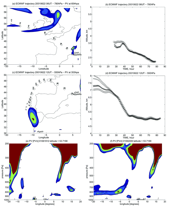Fig. 9 Cluster of 5 backward air mass trajectories ending near Marseille on 22/06/2001 for two rich layers observed by the lidar at 2.5 km, 6 UT (a,b) and at 5 km, 12 UT (c,d). The air mass position is plotted every 6 h and the time scale is set to 0 on 19/06 0 UT for the time–altitude plot. The area with PV values larger than 1, 1.2, 1.5 and 2 PVu are shown for the time and altitude corresponding to the air mass position at the starting point of the trajectory (a,c). The lowest panels (e,f) are the PV vertical cross-sections at the latitude 54° N on 19/06 12 UT and 20/06 06 UT with the same PV contour values as for (a,c).

5.3 Discussion

Comparing both ways of mapping pollution, a ground-based lidar was more beneficial than an airborne lidar because the diurnal evolution of the ozone distribution and the observation of the isolated O₃ rich layers is probably more important for model validation than the O₃ plume horizontal extent at a given time. Indeed a first estimate of the horizontal extent of the O₃ plume can be estimated reasonably well by the in-situ measurements of a research aircraft, especially if forecast of the plume position is provided as it is often the case nowadays.³² Furthermore operating the aircraft for a full chemical characterization of the plume can be achieved at the same time, but it is not the case when the lidar is mounted in the aircraft since lidar operation requires flying above the polluted layer. Nevertheless the analysis of the O₃ horizontal inhomogeneity as observed above Milano is not easy to detect without the airborne lidar mapping. Should such an objective be mandatory, then operation of an airborne lidar for pollution mapping is recommended. If a network of several ground-based lidar (more than 5) can be implemented like during the ESCOMPTE campaign, the same objective could be achieved without an airborne lidar. During a large joint field experiment like ESCOMPTE, the possibility of combining O₃ lidar profiles with wind profiler measurements (Doppler radar or lidar) is quite interesting either for the analysis of the O₃ layer origin or for deriving new parameters like the O₃ fluxes across a given boundary.^22,23 Again the ground-based operation of the O₃ lidar is better adapted to this strategy.

One can add some technical comments when comparing both lidar operations: (1) PBL aerosol interference is less severe for a ground-based operation where the O₃ profile is derived with the most favorable wavelength pair (266/289 nm) while it is not always the case for an aircraft flying near 2000 m. (2) The lidar signal can be averaged over 10 min without decreasing the amount of information about the meso-scale processes controlling the O₃ concentrations but airborne operation must keep the integration time below 2 min reducing then the data quality.

6 Conclusion

The aim of this paper was neither to describe the technical details of the lidar system nor to provide a comprehensive analysis of case studies where the lidar was used.

The first objective was to identify the typical measurement characteristics from comparison with other standard techniques for O₃ profiling. The numerous comparisons that we have performed during several measurement campaigns, clearly show that the O₃ lidar data quality is good enough to identify layers with a 5 to 10 ppb accuracy in the troposphere with a vertical resolution ranging from 200 m to 700 m. In the free troposphere it proved to be a very reliable measurement (except within the clouds) because the aerosol interference can be made small enough. For the PBL, the latter is potentially important, but the lidar data obtained for two different polluted cities do not show large uncertainties in the PBL especially when O₃ retrieval can be performed with the wavelength pair 266/289 nm.

The second objective was to provide some recommendations about O₃ lidar application based on our past experience. Four conclusions have been identified:

(1) lidar remote sensing is mandatory if highly inhomogeneous O₃ fields must be characterized with both a good vertical (< 500 m) and temporal (< 1 h) resolution. This is now well recognized for a quantitative estimate of stratosphere–troposphere exchanges.

(2) Flying together a lidar for O₃ rich layer altitude identification and an aircraft making in-situ measurements of many chemical compounds in the layer puts the aircraft chemical data in a wider perspective by providing the three-dimensional structure of the layer. As far as the aircraft field campaign is concerned, the lidar data are complementary to numerical chemical forecasting for flight planning and is likely to become a standard way to improve the chemical characterization of narrow O₃ layers in the free troposphere. Understanding of the layer life cycle is indeed important considering their contribution to the overall ozone mean concentration.

(3) The use of our lidar system during two field campaigns designed to study the PBL O₃ budget have shown that ozone rich layers are frequently observed above the PBL. The low aerosol load in this region ruled out a strong interference by aerosol particles and these layers are also observed by balloon borne ozonesondes. A preliminary analysis of their origin points both toward meso-scale dynamical processes redistributing O₃ from the PBL, e.g. the Milano experiment, and transport of fossil layers from regions of active stratosphere–troposphere exchanges, e.g. the ESCOMPTE experiment.

O₃ mapping of the polluted PBL is possible from an aircraft but the optimum use of the O₃ lidar remains the continuous operation of a ground-based instrument in combination with wind measurements over a full diurnal cycle. Indeed this gives a better insight into the link between the air mass circulation and the ozone observations considering that it is more difficult to rely on models only in order to identify either complex circulations (orographic influences, land/sea breeze, heat island effect) or the transport of narrow layers from regions of active stratosphere–troposphere exchanges.

Acknowledgements

The OHP lidar station, CNES staff and Instituto Nacionale Meteorologia, Spain (E. Cuevas) are acknowledged for providing ECC data for comparison with the lidar. The Fraunhofer Institut für atmosphärische Umweltforschung (W. Junkermann) and the UK Meteorological Office aircraft facility are acknowledged for providing the aircraft in-situ measurements for comparison with the lidar. Enel, Milano and PSI, Zürich are acknowledged for providing the O₃ profiles during the Milano experiment. ECMWF is acknowledged for providing the meteorological analysis used for trajectory calculations and PV maps.

References

1. N. Harris, G. Ancellet, L. Bishop, D. Hofmann, J. Kerr, R. McPeters, M. Prendez, W. Randel, J. Staehelin, B. Subbaraya, A. Volz-Thomas, J. Zawodny and C. Zerefos, J. Geophys. Res., 1997, 102, 1571–1590.
2. S. Godin, A. Carswell, D. Donovan, H. Claude, W. Steinbrecht, I. McDermid, T. McGee, M. Gross, H. Nakane, D. Swart, H. Bergwerff, O. Uchino, P. von der Gathen and R. Neuber, Appl. Opt., 1999, 38, 6225–6236.
3. H. Eisele, H. Scheel, R. Sladkovic and T. Trickl, J. Atmos. Sci., 1999, 56, 319–330.
4. S. Bethan, G. Vaughan, C. Gerbig, A. Volz-Thomas, H. Richer and D. Tiddeman, J. Geophys. Res., 1998, 103(13), 413–434.
5. E. Browell, in Optical Laser Remote Sensing, eds. D. K. Dillinger and A. Mooradian, Springer-Verlag, New York, 1983, pp. 138–147.
6. D. A. Richter , E. V. Browell , C. F. Butler and N. S. Higdon, in Advances in Atmospheric Remote Sensing with Lidar, ed. A. Ansmann, Springer-Verlag, New York, 1997, pp. 395–398.
7. E. V. Browell, S. Ismail and W. B. Grant, Appl. Phys. B, 1998, 67, 399–410.
8. J. Raper, M. Kleb, D. Jacob, D. Davis, R. Newell, H. Fuelberg, R. Bendura, J. Hoell and R. McNeal, J. Geophys. Res., 2001, 106(32), 401–425.
9. H. Moosmüller, R. Alvarez II, C. M. Edmonds, R. M. Jorgensen, D. H. Bundy and J. L. McElroy, Opt. Remote Sens. Atmos. Tech. Digest, 1993, 5, 176–179.
10. R. Banta, C. Senff, A. White, M. Trainer, R. McNider, R. Valente, S. Mayor, R. Alvarez II, R. Hardesty, D. Parrish and F. Fehsenfeld, J. Geophys. Res., 1998, 103(22), 519–544.
11. G. Ancellet and F. Ravetta, Appl. Opt., 1998, 37, 5509–5521.
12. J. Bösenberg, G. Ancellet, R. Barbini and M. Milton, in Instrument Development for Atmospheric Research and Monitoring, eds. J. Bösenberg, D. Brassington and P. Simon, Springer, Berlin, FRG, 1997, pp. 1–204.
13. A. Papayannis, G. Ancellet, J. Pelon and G. Megie, Appl. Opt., 1990, 29, 467–476.
14. E. Browell, S. Ismail and S. Shipley, Appl. Opt., 1985, 24, 2827–2836.
15. Committe on Extension of the Standard Atmosphere C, U.S. Standard Atmosphere, NOAA, Washington, DC, USA, 1976.
16. P. Völger, J. Bösenberg and I. Schult, Contrib. Atmos. Phys., 1996, 69, 177–187.
17. J. Kowol-Santen and G. Ancellet, Geophys. Res. Lett., 2000, 27, 3345–3348.
18. E. Browell, J. Geophys. Res., 1987, 92, 2112.
19. F. Ravetta and G. Ancellet, Mon. Weather Rev., 2000, 128, 3252–3267.
20. E. Browell, M. Fenn, C. Butler, W. Grant, J. Merrill, R. Newell, J. Bradshaw, S. Sandholm, B. Anderson, A. Randy, A. Bachmeier, D. Blake, D. Davis, G. Gregory, B. Heikes, Y. Kondo, S. Liu, F. Rowland, G. Sachse, H. Singh, R. Talbot and D. Thornton, J. Geophys. Res., 1996, 101, 1691–1712.
21. E. Browell, M. Fenn, C. Butler, W. Grant, S. Ismail, R. Ferrare, S. Kooi, V. Brackett, M. Clayton, M. Avery, J. Barrick, H. Fuelberg, J. Maloney, R. Newell, Y. Zhu, M. Mahoney, B. Anderson, D. Blake, W. Brune, B. Heikes, G. Sachse, H. Singh and R. Talbot, J. Geophys. Res., 2001, 106(32), 481––501.
22. C. Senff, R. Alvarez II, S. D. Mayor and Y. Zhao, in Advances in Atmospheric Remote Sensing with Lidar, ed. A. Ansmann, Springer-Verlag, New York 1997, pp. 363–366.
23. R. M. Hardesty, C. Senff, W. Brewer, R. Banta, R. Alvarez II, L. Darby and R. Marchbanks, in Advances in Atmospheric Remote Sensing with Lidar, ed. A. Dabas, Editions de l'Ecole polytechnique, 2001, pp. 451–454.
24. K. R. Mulik and C. R. Philbrick, Advances in Atmospheric Remote Sensing with Lidar, ed. A. Dabas, Editions de l'Ecole polytechnique, 2001, pp. 443–446.
25. B. Calpini, in Advances in Atmospheric Remote Sensing with Lidar, ed. A. Dabas, Editions de l'Ecole polytechnique, 2001, pp. 427–429.
26. P. Quaglia, O. Couach, J. Balin, V. Simeonov, B. Lazzarotto, H. V. den Bergh and B. Calpini, in Advances in Atmospheric Remote Sensing with Lidar, ed. A. Dabas, Editions de l'Ecole polytechnique, 2001, pp. 435–438.
27. A. Thomasson, D. Mondelain, J. Yu, J. P. Wolf, E. Frejafon, P. Viscardi, P. Ritter, T. Menard, Y. Godet, D. Weidauer, R. Fabian, V. Schmidt and D. Moeller, in Advances in Atmospheric Remote Sensing with Lidar, ed. A. Dabas, Editions de l'Ecole polytechnique, 2001, pp. 431–434.
28. T. Staffelbach, A. Neftel, A. Blatter, A. Gut, M. Fahrni, J. Stähelin, A. Prévot, A. Hering, M. Lehning, B. Neininger, M. Bäumle, G. Kok, J. Dommen, M. Hutterli and M. Anklin, J. Geophys. Res., 1997, 102(23), 345–362.
29. T. Staffelbach, A. Neftel and L. Horowitz, J. Geophys. Res., 1997, 102(23), 363–373.
30. J. Donnadille, J. Cammas, P. Mascart, D. Lambert and R. Gall, Q. J. R. Meteorol. Soc., 2001, 127, 2247–2268.
31. G. Gangoiti, M. Millán, R. Salvador and E. Mantilla, Atmos. Environ., 2001, 35, 6267–6276.
32. L. Menut, R. Vautard, C. Flamant, C. Abonnel, M. Beekmann, P. Chazette, P. Flamant, D. Gombert, D. Guédalia, D. Kley, M. Lefebvre, B. Lossec, D. Martin, G. Mégie, P. Perros, M. Sicard and G. Toupance, Ann. Geophys., 2000, 18, 1467–1481.

---