Chemical rank estimation by noise perturbation in functional principal component analysis†
Cheng-Jian
Xu
a,
Yi-Zeng
Liang
*a,
Yang
Li
b and
Yi-Ping
Du
b
aCollege of Chemistry and Chemical Engineering, Institute of Chemometrics and Intelligent Analytical Instruments, Central South University, Changsha 410083, P.R. China. E-mail: yzliang@public.cs.hn.cn; Fax: 86-731-8825637; Tel: 86-731-8822841
bCollege of Chemistry and Chemical Engineering, Hunan University, Changsha 410082, P.R. China
First published on 10th December 2002
Abstract
Some kinds of chemical data are not only univariate or multivariate observations of classical statistics, but also functions observed continuously. Such special characters of the data, if being handled efficiently, will certainly improve the predictive accuracy. In this paper, a novel method, named noise perturbation in functional principal component analysis (NPFPCA), was proposed to determine the chemical rank of two-way data. In NPFPCA, after noise addition to the measured data, the smooth eigenvectors can be obtained by functional principal component analysis (FPCA). The eigenvectors representing noise are sensitive to the perturbation, on the other hand, those representing chemical components are not. Therefore, by comparing the difference of eigenvectors obtained by FPCA with noise perturbation and by traditional principal component analysis (PCA), the chemical rank of the system can be achieved accurately. Several simulated and real chemical data sets were analyzed to demonstrate the efficiency of the proposed method.
Introduction
In the last two decades, there has been an upsurge of interest and activity in the modern hyphenated analytical instruments. These instruments are capable of providing two-dimensional bilinear data.1 For instance, the data produced by hyphenated chromatography can be formulated as a matrix X of size m × n, where the m rows are absorption spectra measured at regular time intervals and the n columns are chromatograms measured at different wavelengths.The first important step for handling this kind of data is to determine the number of chemical components in the mixtures.2 An incorrect estimation of that will give misguidance for further qualitative and quantitative analysis. The number of components in the mixtures, usually called ‘chemical’ rank of the measured matrix,3 has a good one-to-one correspondence relation with the number of significant singular values of the data matrix X, provided that the spectra profiles of the components are linearly independent of each other.
It seems that chemical rank estimation is an easy task, however, practical experimental errors, such as uncorrected background, instrumental noise and low signal to noise ratio, make it very difficult in practice. Therefore, many kinds of statistical and empirical methods were proposed to resolve this problem.4–10
Most rank-estimation methods are based on principal component analysis (PCA). These methods can be roughly classified into two representative categories. The former is based on eigenvalue analysis, and the typical representation is Malinowski’s F-test or indicator function (IND).4 The latter is focused on frequency domain analysis5 in eigenvector analysis. The reason is that the frequency of the spectral profiles often appears low, whilst on the contrary, that of the noise usually appears high.
Meloun et al. gave a good critical review and comparison of many methods predicting the number of components in spectroscopic data.2 They came to the conclusion that in case of real experimental data, the RESO (the ratio of eigenvalues calculated smooth PCA and those calculated by ordinary PCA),6 IND and those indices methods based on knowledge of instrumental error should be preferred. To our knowledge, it will be wiser to use different methods according to different prior chemical information. The prior chemical information includes different kinds of data sets, instrumental noise level and so on. For instance, if the knowledge of instrumental error is known beforehand, the methods based on it should be preferred.2 When the responsive profiles are smooth, the frequency domain analysis, the morphological approach,7 or RESO could be chosen. If the responsive profiles have an evolving character11 the pure variable12 methods, such as Simplisma (simple-to-use iterative self-modeling mixture analysis),12 OPA (orthogonal projection approach)13 or other local rank estimation method14 are preferred. In our opinion, the performance of rank estimation methods has a strong relationship with the consistency of the model assumption and the property of real systems. Therefore, to develop different methods corresponding to different kinds of chemical data sets seems a promising job.
Chemical observation data, such as ultraviolet, fluorescence and some electrochemistry response etc., often appear as a continuous function of wavelength or potential. Such special characters of data, if being handled efficiently, will certainly improve the predictive accuracy. Functional data analysis, firstly proposed by Ramsay and Dalzell,15 then developed by Silverman and co-workers16,17 is a nonparametric method involving smooth in some way. In this paper, a novel rank estimation method, called noise perturbation in functional principal component analysis (NPFPCA), was proposed to determine the chemical rank of two-way data. In NPFPCA, after noise addition to the measured data, the eigenvectors can be obtained by functional principal component analysis (FPCA). Since the FPCA focuses more on systematic effects and less on random effects in the data, the eigenvectors representing noise are sensitive to the noise perturbation, whereas those representing chemical components are nearly unaffected by the noise perturbation. Then, by comparing the difference of eigenvectors obtained by FPCA and by traditional principal component analysis (PCA), the number of components in the concerned system can be estimated accurately.
The noise perturbation method proposed in this paper has some similar features with the data augmentation technique18 and smoothed bootstrap method.19 The former one uses noise addition to obtain sufficient relevant data to enable an accurate and robust calibration model, and the latter one uses a smooth estimate of the distribution instead of the empirical estimate.
Conclusions inferred from the theoretical study are used afterwards to clarify the performance of the proposed method on the simulated and real examples and to provide some general guidelines to understand better the potential of our method.
Method
Notation
Suppose that there is a given measured data matrix X of size m × n, and there are p components in mixture (p ⩽ min(m,n)). Matrices are denoted by bold capital letters and vectors by bold lowercase letters. The superscript T denotes the matrix or vector transposition. In this paper, only a discretion version of roughness penalty is adopted.16,17 Here, [r,r] is defined as the roughness penalty of discrete function r(t) and [r,r] equals rTQr, where Q = GTG, and G is a second difference matrix.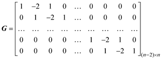 | (1) |
Principal component analysis (PCA) and functional principal component analysis (FPCA)
Principal components analysis (PCA), which has a good ability to summarize multivariate variation in data, is a popular method in applied statistical work and data analysis.20 PCA is used to find a set of orthogonal normalized vectors ri (i = 1, 2,…, n) by maximizing the following criterion| λi = rTiXTXri (i = 1, 2,…, n) | (2) |
Here δi,j is the Kronecker delta, and ri is the ith eigenvector of covariance matrix XTX associated with eigenvalue λi. Let the eigenvectors of XTX be numbered according to the magnitude of the eigenvalues λ1
![[greater than or equal, slant]](https://www.rsc.org/images/entities/char_2a7e.gif) λ2
λ2
![[greater than or equal, slant]](https://www.rsc.org/images/entities/char_2a7e.gif) …
…
![[greater than or equal, slant]](https://www.rsc.org/images/entities/char_2a7e.gif) λn, then
λn, then ![[x with combining tilde]](https://www.rsc.org/images/entities/b_i_char_0078_0303.gif) i = Xri is the ith principal component.
i = Xri is the ith principal component.
Assuming the rank of matrix X is p with p ⩽ min(m,n), in exact multicollinearity situation, we get
| λn − p + 1 = … = λn = 0 | (3) |
In chemical systems, the rank can be determined by observing the significant eigenvalues by PCA of the data matrix XTX. Here, only the variance is considered for rank estimation. Although the size of variance is important for rank estimation, other characters of chemical data are also useful, which will lead to a more satisfactory result. For example, chemical observations often have a special property, that is, they often appear as smooth and continuous function of wavelength or potential. As they are linear combinations of original variables, the principal components representing chemical spectra signals are also smooth. Such special characters of data, if being utilized efficiently, will certainly enhance the predictive accuracy of rank estimation. Chen et al. first introduced the FPCA into chemistry.6 The roughness penalty is the key idea of FPCA, which is to find a set of orthogonal normalized vector rfi (i = 1, 2, …, n) by maximizing the following criterion
 | (4) |
Here δi,j is the Kronecker delta, rfi is the ith smooth eigenvector of matrix XTX associated with smooth eigenvalue λfi , and α is positive smooth parameter regulating the trade-off between the fidelity of measured data and roughness. The smoothing parameter α can be chosen subjectively or by cross-validation.16
In fact, smooth eigenvector rfi and smooth eigenvalue λfi can be obtained by solving following generalized eigenvalue problem.
| XTXrfi = λfi(I + αQ)rfi (i = 1, 2, …, n) | (5) |
| BXTXrfi = λfirfi (i = 1, 2, …, n) | (6) |
The matrix BXTX is of size n × n but not symmetric. Rather than finding its eigenvectors directly it may be easier to proceed as follows, solving a symmetric matrix XBXT problem instead.
Let ci be an eigenvector of XBXT with eigenvalue μi. Then it is easy to show that
| wi = BXTci | (7) |
In implementing the methods, we have used a singular value decomposition (SVD) of matrix XB1/2 to find eigenvector wi of matrix XBXT.
Rank estimation by noise perturbation in functional principal component analysis
In fact, the eigenproblem of eqn. (5) can be considered as a perturbation of the eigenproblem of eqn. (2).17Table.1 shows the ratio between the ith eigenvalues of PCA and FPCA of a three-component simulated system. The spectra and chromatographic profiles of the system are shown in Fig. 1. It is difficult to directly draw a conclusion that the true component number is three from the ratio between eigenvalue of PCA and FPCA. The third ratio of eigenvalue is about 0.8. It is hard to say that when the ratio is bigger than 0.8, the corresponding eigenvectors definitely represent a signal. This is because the result may occur by accident. Chen et. al. suggested that rank estimation could be obtained by observing the ratio change with the variation of smooth parameter α. However, a small change of α can not distinguish noise from signals. For example, as seen in the Table 1, when α is changed from 1 to 1.1 all eight eigenvalues remain almost unchanged. On the contrary, a great variation in α will make the small eigenvalues representing chemical components also change significantly. It is difficult to determine the component number in such a case. As shown in Table 1, the third eigenvalue changed from 0.8775 to 0.8486 when α changed from 1 to 10. It is hard to say that the third eigenvalue corresponds to a chemical component. In our opinion, a great change in α seems unsuitable since there is a trade-off between curve fitting (under-smoothing) and curve distortion (over-smoothing) in any smoothing process.21| λ f i /λoi (α = 1) | λ f i /λoi (α = 1.1) | λ f i /λoi (α = 10) | C (α = 1) | C (α = 1 noise) | |
|---|---|---|---|---|---|
| 1 | 1.0000 | 1.0000 | 0.9998 | 1.0000 | 1.0000 |
| 2 | 0.9988 | 0.9987 | 0.9889 | 1.0000 | 1.0000 |
| 3 | 0.8775 | 0.8760 | 0.8486 | 0.9362 | 0.9336 |
| 4 | 0.5745 | 0.5676 | 0.4599 | 0.2633 | 0.3036 |
| 5 | 0.5446 | 0.5412 | 0.4305 | 0.0489 | 0.0665 |
| 6 | 0.5430 | 0.5341 | 0.4157 | 0.3904 | 0.3538 |
| 7 | 0.5486 | 0.5402 | 0.4097 | 0.2327 | 0.1187 |
| 8 | 0.5224 | 0.5155 | 0.3841 | 0.2448 | 0.0568 |
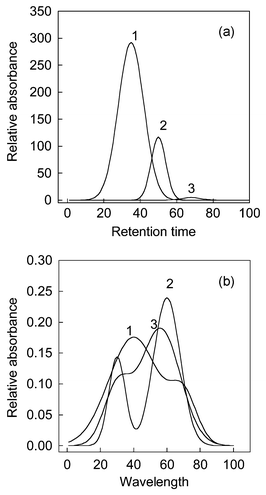 | ||
| Fig. 1 (a) The chromatographic profile and (b) spectra of a three-component simulated system. | ||
Under this consideration, artificial random noise, instead of great changes in the smooth parameter α, are added to the original measured matrix. It should be noted that the added artificial noises are small in order not to influence the model of the original data. In FPCA, the degree of roughness of eigenvectors is also considered beside the variance. Therefore, the smooth chemical signals are extracted in FPCA before random noise in the data. The added artificial Gauss noise, which is of course not smooth, will certainly give little contribution to the smooth principal components representing spectra signal. On the other hand, the added artificial noise changes the structure of original noise; therefore, the smooth eigenvectors representing noise will change dramatically.
Therefore, by comparing the space spanned by the eigenvectors of PCA and those of FPCA, the chemical rank of the mixture can be obtained thereafter.
| Ck = rTkrfk (k = 1, 2, …, n) | (8) |
Here Ck is called congruence coefficient of the kth eigenvectors. If Ck is nearly to 1, and Ck+1 ≪ 1, then the rank (X) = k.
The third congruence coefficient of the eigenvectors Ck is bigger than 0.9, but it is still not convincing to regard it as chemical component, as this may take place by accident. When different artificial noises are added in different experiments, if the third congruence coefficient remains rather stable, we can draw a safer conclusion that the third eigenvector represents the chemical component.
A Monte-Carlo simulation is used here to study the change of eigenvectors with different random added noises. The same level of noise, produced by different random seeds, is added to the same measured matrix. Then we can calculate the standard deviation of Ck as follows.
 | (9) |
From another point of view, the above noise addition procedure can be regarded as many parallel experiments aiming for a same job. In analytical experiments, the random noises of parallel experiments are also different. If the added noises do not influence the structure of raw data, a constant rank estimation result will certainly be obtained.
In this paper, the comparison of eigenvectors, instead of eigenvalue, was chosen here for rank estimation. The reason is as follows: firstly, for a system containing minor components, the eigenvectors can provide more information than eigenvalues.22 Secondly, in the case of smooth column and row space, the rank estimation can be achieved by calculating not only the eigenvectors representing column space but also those representing row space. Results obtained by these two procedures can provide interrelated and validated information together. Furthermore, the eigenvectors representing column space and row space are not necessary all smooth. Only one smooth kind of them is enough to use the NPFPCA methods for rank estimation.
Experimental
All programs were written in Matlab 5.3 environment. Matlab program was executed on a Pentium III 850(Intel) personal computer with 192MB RAM under the Microsoft Windows 98 operating system. The NPFPCA was tested and compared to established criteria with three different types of data: a three-component simulation, HPLC-DAD pesticide data and GC-MS traditional Chinese medicine data. The program implementing the algorithm in this paper is available from the author (see electronic supplementary information (ESI))†.Simulated data
Firstly, a simulated three-component data set was selected to demonstrate the procedure of NPFPCA method. Homoscedastic noise with standard deviation 0.2% of the maximum absorbance was added to construct the measurement data set. Then homoscedastic noise with standard deviation 0.03% of the maximum absorbance is added each time as a perturbation to show the procedure of the proposed method. Then the variation in concentration, noise level, the kind of noise, and collinearity of spectra was constructed to show the performance of the proposed method.Concentration variation
One of the components in system was arranged at different concentration levels, actually 0.003, 0.005, 0.01, 0.02 and 0.05 of sum of the other two components in system. Homoscedastic noise with standard deviation 0.05% of the maximum absorbance was added.Homoscedastic noise
The components in the system were arranged at 0.01 of the sum of the other two components. Normally distributed noise with zero expectation and different standard deviation from 0.03% to 0.2% of the maximum absorbance was added.Heteroscedastic noise
The heteroscedastic noise was generated by the addition of two kinds of noise. The first one is homoscedastic noise with standard deviation of 0.01%, and the second noise is proportional to the absorbance, the proportionality factor23β is from 2 to 10. The concentration level is the same as that in homoscedastic noise.Collinearity in spectra
In this case, the concentration level is the same as that in homoscedastic noise. Normally distributed noise with zero expectation and different standard deviation 0.1% of the maximum absorbance was added. With the change of the spectra component 3, the correlation coefficient between component 3 and component 2 varied from 0.90 to 0.999.HPLC-DAD pesticide data
The liquid chromatographic data for pesticide determinations were measured with DAD in the range 200–248 nm with a spectral resolution of 2nm. Five-component sample consisted of 4 ppm of iprodione, 2 ppm of procymidone, 4 ppm of chlorothalonil, 6 ppm of folpet (N-(trichloromethylthio)phthalimide) and 5 ppm of triazophos (O,O-diethyl O-1-phenyl-1H-1,2,4-triazol-3-yl phosphorothioate), respectively (see ref. 24 for more details).GC-MS Chinese medicine data
A little fraction of the GC-MS data analyzing the essential constituents of Ramulus cinnamomi was selected. There are three components in the system, named 2-methyl-heptane, 1-methylethyl-benzene, and 2,4-dimethyl-hexane. The extensive experimental condition can be seen in ref. 25.Results and discussion
Two important parameters
To implement the NPFPCA method, two important parameters should be ascertained beforehand. One is positive smooth parameter α and the other is the level of added noise.As mentioned before, smooth parameter α can be chosen by cross-validation or subjectively. In fact, a subjective choice of smoothing parameter is satisfactory or even preferable in many problems.17 Therefore, smooth parameter 1 is selected in the all experiments. In our experience, too big or too small a parameter is often not suitable. We choose a parameter usually between 1 and 10.
The level of noise is also another important parameter. In this paper, a Gauss noise is selected as a perturbation noise. In general, the level of noise chosen is not too high to change the structure of data set. Too much noise submerges the minor component, and indeed changes to the structure of original data set will give us a misleading result. On the other hand, too small noise will not give us enough perturbation. In general, if the added noise is around instrumental error, the proposed method can give us a satisfactory result. In all experiments, one experiment did not have added noise. By observing the difference between the one experiment without added noise with others, one can discern how added noise influences the result of rank estimation, whether the added noise changes the structure of original data or the added noise is big enough to perturb.
To our knowledge, the performance of the NPFPCA method is usually not sensitive to the level of noise, which is attractive in practice. On the other hand, one can try different levels of noise to obtain a stable and satisfactory result.
A three-component simulated data
The chromatographic profiles and spectra of the simulated system are shown in Fig. 1. We name the components according to their elution order, and they are components 1, 2 and 3 respectively. Firstly, the data matrix is decomposed by SVD. The first ten eigenvectors, which spanned the spectral space, are selected. Then, we decompose the data matrix by FPCA and smooth parameter α is equal to 1 here. The first ten smooth eigenvectors are selected too. By comparison with eigenvectors obtained by PCA and FPCA, congruence coefficient of eigenvector Ckversus increasing estimated component number from one to ten is shown in Fig. 2. From this figure, it can be seen that a little decline appeared as the component number changed from 2 to 3, whereas a sharp decline appeared from 3 to 4. We usually believe that the component number equals 3. Nevertheless, in a real system, a gradual change, which makes rank determination difficult, often appears when the estimating number increases. Consequently, same levels of noise generated by different random seeds are added into the original data set. Since the smooth signal are usually unaffected by this perturbation, a stable result can be obtained. We plotted the standard deviation of the congruence coefficient of eigenvectors Ckversus increasing component number, which is displayed in Fig. 3. There are in total 100 experiments, and noise is added in ninety-nine of them. By observing the difference between the one experiment without additional noise and the others, one can discern how the added noise influences the result in rank estimation, and whether the added noise changes the structure of original data or the added noise is big enough. If the Ck obtained without added noise is apparently different to that obtained with added noise, one can change the level of noise to obtain a good result. In Fig. 3, a flat line from component numbers 1 to 3 and a sharp increase from 3 to 4 point out that the true chemical rank is three.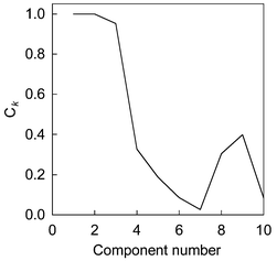 | ||
| Fig. 2 The congruence coefficient of eigenvector (Ck) versus component number. | ||
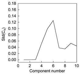 | ||
| Fig. 3 The standard deviation of congruence coefficient of eigenvectors (Ck) versus increasing estimated component number in a simulated system. | ||
Comparison with other traditional indices
Four other empirical indices,4,6 IE (imbedded error), IND, ER (eigenvalue ratio) and VPVRS (variance percentage to variance sum) are selected to compare with the NPFPCA method. The definition of these four indices is shown as follows.Use the SVD to find the eigenvalue λi (i = 1, 2, …, n, assuming m > n) of covariance matrix XTX and do the following calculations.
 | (10) |
 | (11) |
 | (12) |
 | (13) |
Here m and n are the number of rows and columns of measured matrix X respectively.
The effect of concentration, noise and spectra collinearity on rank estimation of five indices has been shown in Tables 2–5. An inspection of the results in Tables 2 to 5 reveals that the NPFPCA method performed well with great variation in concentration level, noise level, and degree of collinearity and pattern of noise. In both cases, there are fewer components than desired and than identified by IE, ER and VPVRS. The reason is that these indices are often not sensitive enough; when the condition number of matrix is larger, they often regard some minor components as noises. However, IND is sensitive enough to detect components in low concentrations and high levels of homoscedastic noises situation. But in heteroscedastic noise, IND works rather badly. It regards heteroscedastic noise as components.
| Concentration | IE | IND | ER | VPVRS | NPFPCA |
|---|---|---|---|---|---|
| 0.003 | 2 | 3 | 2 | 2 | 3 |
| 0.005 | 2 | 3 | 2 | 2 | 3 |
| 0.010 | 3 | 3 | 2 | 2 | 3 |
| 0.020 | 3 | 3 | 2 | 3 | 3 |
| 0.050 | 3 | 3 | 3 | 3 | 3 |
| Noise level | IE | IND | ER | VPVRS | NPFPCA |
|---|---|---|---|---|---|
| 0.0002 | 3 | 3 | 2 | 2 | 3 |
| 0.0005 | 3 | 3 | 2 | 2 | 3 |
| 0.0010 | 2 | 3 | 2 | 2 | 3 |
| 0.0015 | 2 | 3 | 2 | 2 | 3 |
| 0.0020 | 2 | 3 | 2 | 2 | 3 |
| β | IE | IND | ER | VPVRS | NPFPCA |
|---|---|---|---|---|---|
| 2 | 3 | 3 | 2 | 2 | 3 |
| 4 | 3 | 7 | 2 | 2 | 3 |
| 6 | 3 | ![[greater than or equal, slant]](https://www.rsc.org/images/entities/char_2a7e.gif) 10 10 |
2 | 2 | 3 |
| 8 | 3 | ![[greater than or equal, slant]](https://www.rsc.org/images/entities/char_2a7e.gif) 10 10 |
2 | 2 | 3 |
| 10 | 3 | ![[greater than or equal, slant]](https://www.rsc.org/images/entities/char_2a7e.gif) 10 10 |
2 | 2 | 3 |
| Correlation coefficient | IE | IND | ER | VPVRS | NPFPCA |
|---|---|---|---|---|---|
| 0.900 | 2 | 3 | 2 | 2 | 3 |
| 0.950 | 2 | 3 | 2 | 2 | 3 |
| 0.970 | 2 | 3 | 2 | 2 | 3 |
| 0.990 | 2 | 3 | 2 | 2 | 3 |
| 0.999 | 2 | 3 | 2 | 2 | 3 |
IND usually works well when the noise pattern is homoscedastic, which is consistent with the model assumption of IND method. The other three indices often can not acquire stable and satisfactory results.
Real data
In five-component pesticide data, noise perturbation approaches were carried out 100 times. Noise is added in 99 experiments but in one noise is omitted. The plot Ck with increasing component number can be seen in Fig. 4a. For simplicity and explicitness, only the results of 10 experiments are shown in Fig. 4(a). In Fig. 4(a), the Ck remained very stable when k increases from one to five. On the contrary, when the estimated component number is bigger than five, the Ck varied greatly. The biggest value of C6 is 0.9017, the smallest value of C6 is 0.3622, and the value of C6 without noise perturbation is 0.8744. From the above numerical value, we can conclude that the value of C6 is not stable with added noise. A high numerical value of Ck obtained once, for example, 0.9017, is not reliable for rank estimation, which occur by accident. Therefore, after 100 experiments with noise perturbation, we plotted the standard deviation of Ckversus increasing component number, then the chemical rank of real system can be obtained in a statistical sense. The results were displayed in Fig. 4(b). In all experiments, the smooth parameter α is chosen as 1 subjectively, and the added noise is normally distributed with zero expectation and 0.1% of the maximum absorbance. Here only the smooth information in spectra space is used. In fact, the eigenvectors in chromatographic space can also provide the same satisfactory results. It is very easy to implement this method in row space. One can use the transpose of measured matrix X instead of matrix X. Therefore, the eigenvectors in column and row space can provide a self-validated information together.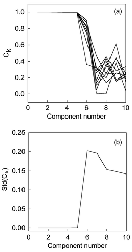 | ||
| Fig. 4 (a) The congruence coefficient of eigenvector (Ck) versus component number for 10 computation. (b) The standard deviation of congruence coefficient of eigenvectors (Ck) versus increasing estimated component number in pesticide system. | ||
Another attractive characteristic of the proposed method is that it can also be used to deal with GC-MS data, In contrast, the RESO algorithm often can not tackle it.6 Since functional data analysis has an assumption that the data are continuous and smooth, it can not be applied to bar-like mass spectra data. However, the NPFPCA method can achieve a result from chromatographic space, rather than mass spectra space, because chromatographic space often appears smooth and continuous. The final results are displayed in Fig. 5. Moreover, the rank estimation results by five other indices are summarized in Table 6. The indices IND, IE, ER and VPVRS can not usually obtain satisfactory results in real systems.
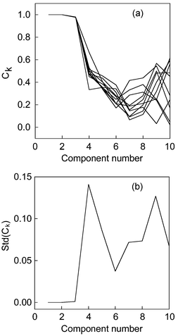 | ||
| Fig. 5 (a) The congruence coefficient of eigenvector (Ck) versus component number in chromatographic space versus increasing estimated component number for 10 computations. (b) The standard deviation of congruence coefficient of eigenvectors (Ck) in chromatographic space versus increasing estimated component number in Chinese medicine system. | ||
| Sample | IE | IND | ER | VPVRS | NPFPCA |
|---|---|---|---|---|---|
| Pesticide | ![[greater than or equal, slant]](https://www.rsc.org/images/entities/char_2a7e.gif) 10 10 |
7 | 5 | 5 | 5 |
| Chinese medicine | 2 | ![[greater than or equal, slant]](https://www.rsc.org/images/entities/char_2a7e.gif) 10 10 |
1 | 1 | 3 |
It should be noted that it is usually safe to combine the congruence coefficient of eigenvectors and its standard deviation plot. If the congruence coefficient is near to 1, and its standard deviation is also near to zero, then this eigenvector represents chemical signal.
Conclusion
The main idea of proposed NPFPCA method is adding an artificial random noise in FPCA. The FPCA is distinguished from statistical methods because it focuses more on systematic effects and less on random effects in the data. Therefore, even in different noise situations, the smooth eigenvectors representing spectra are usually unaffected, however, the eigenvectors representing noise are usually sensitive to the perturbation. Combining the congruence coefficient of eigenvectors and its standard deviation plot, a safe chemical rank can usually be obtained. The proposed method can be regarded as many parallel tests on the same data set. It will give us a reasonable result in a statistical sense.Acknowledgements
The authors would like to thank Prof. D. L Massart for providing the HPLC-DAD pesticide data. This work was financially supported by the National Natural Science Foundation of the People’s Republic of China (Grant No 20175036).References
- T. Hirschfeld, Anal. Chem., 1980, 52, 297–303A.
- M. Meloun, J. Capek, P. Miksik and R. G. Brereton, Anal. Chim. Acta, 2000, 423, 51–68 CrossRef CAS.
- Y. Z. Liang and O. M. Kvalheim, Fresenius’ J. Anal. Chem., 2001, 370, 694–704 Search PubMed.
- E. R. Malinowski, Factor Analysis in Chemistry, Wiley, New York, 2nd edn., 1991 Search PubMed.
- T. M. Rossi and I. M. Warner, Anal. Chem., 1986, 58, 810–815 CrossRef CAS.
- Z. P. Chen, Y. Z. Liang, J. H. Jiang, Y. Li, J. Y. Qian and R. Q. Yu, J. Chemom., 1999, 13, 15–30 CrossRef CAS.
- J. H. Wang, J. H. Jiang, J. F. Xiong, Y. Li, Y. Z. Liang and R. Q. Yu, J. Chemom., 1998, 12, 95–104 CrossRef CAS.
- N. M. Faber, L. M. C. Buydens and G. Kateman, Anal. Chim. Acta, 1994, 296, 1–20 CrossRef CAS.
- R. C. Henry, E. S. Park and C. H. Spiegelman, Chemom. Intell. Lab. Syst., 1999, 48, 91–97 CrossRef CAS.
- B. K. Dable and K. S. Booksh, J. Chemom., 2001, 15, 591–613 CrossRef CAS.
- C. J. Xu, J. H. Jiang and Y. Z. Liang, Analyst, 1999, 124, 1471–1476 RSC.
- W. Windig and J. Guilment, Anal. Chem., 1991, 63, 1425–1432 CrossRef CAS.
- F. C. Sanchez, J. Toft, B. V. D. Bogaert and D. L. Massart, Anal. Chem., 1996, 68, 79–85 CrossRef.
- H. R. Keller and D. L. Massart, Anal. Chim. Acta, 1991, 246, 379–390 CrossRef CAS.
- J. O. Ramsay and C. J. Dalzell, J. R. Statist. Soc. B, 1991, 53, 539–572 Search PubMed.
- P. J. Green and B. W. Silverman, Nonparametric Regression and Generalized Linear Models: A Roughness Penalty Approach, Chapman and Hall, London, 1994 Search PubMed.
- B. W. Silverman, Ann. Statist., 1996, 24, 1–24 Search PubMed.
- A. K. Conlin, E. B. Martin and A. J. Morris, Chemom. Intell. Lab. Syst., 1998, 44, 161–173 CrossRef CAS.
- B. W. Silverman, Density Estimation for Statistics and Data Analysis, Chapman and Hall, London, 1986 Search PubMed.
- T. W. Anderson, An Introduction to Multivariate Statistical Analysis, Wiley, New York, 2nd edn, 1984 Search PubMed.
- Y. Z. Liang, A. K. M. Leung and F. T. Chau, J. Chemom., 1999, 13, 511–524 CrossRef CAS.
- Y. Z. Liang, O. M. Kvalheim, H. R. Keller, D. L. Massart, P. Kiechle and F. Erni, Anal. Chem., 1992, 64, 946–953 CrossRef.
- C. Ritter, J. A. Gilliard, J. Cumps and B. Tilquin, Anal. Chim. Acta, 1995, 318, 125–136 CrossRef CAS.
- F. C. Sanchez, S. C. Rutan, M. D. G. Garcia and D. L. Massart, Chemom. Intell. Lab. Syst., 1997, 36, 153–164 CrossRef CAS.
- C. J. Xu, Y. Z. Liang, Y. Q. Song and J. S. Li, Fresenius’ J. Anal. Chem., 2001, 371, 331–336 Search PubMed.
Footnote |
| † Electronic supplementary information (ESI) available: Program and test data. See http://www.rsc.org/suppdata/an/b2/b205818a/ |
| This journal is © The Royal Society of Chemistry 2003 |
