Examples of the role of analytical chemistry in environmental risk management research

Abstract

Analytical chemistry is an important tier of environmental protection and has been traditionally linked to compliance and/or exposure monitoring activities for environmental contaminants. The adoption of the risk management paradigm has led to special challenges for analytical chemistry applied to environmental risk analysis. Namely, methods developed for regulated contaminants may not be appropriate and/or applicable to risk management scenarios. This paper contains examples of analytical chemistry applied to risk management challenges broken down by the analytical approach and analyte for some selected work in our laboratory. Specific techniques discussed include stable association complex electrospray mass spectrometry (cESI-MS), gas chromatography-mass spectrometry (GC-MS), split-flow thin cell (SPLITT) fractionation and matrix-assisted laser desorption time of flight mass spectrometry (MALDI-ToF-MS). Specific analytes include haloacetic acids (HAA9), perchlorate, bromate, triazine degradation products, metal-contaminated colloids and Cryptosporidium parvum oocysts.

---

1 Introduction

Environmental risk management seeks to prevent and reduce risks from pollution that threaten human health and the environment.¹ For this purpose, it is necessary to develop scientific information to support regulatory and policy decisions across the risk management paradigm. This helps to provide a rigorous, scientifically credible understanding of the complex interactions among environmental stressors, sources, relative risks and risk management alternatives. Fig. 1 shows a diagram of the scientific and technical contributions to the process of risk management.¹ The scientifically credible information needed in Fig. 1 relies on high quality data. Increasingly, as basic environmental issues are better understood, the task of providing high quality data for input into the risk management process has substantially increased in complexity. One such area is the determination of environmental contaminants. Fig. 1 shows many points of input for contaminant determination, particularly in terms of risk assessment, monitoring compliance and measuring improvement. Wet chemical analysis once provided essentially all the data needed for environmental decision making. While many wet chemical methods still provide useful information, the field of environmental analytical chemistry has developed, mainly through advances in analytical instrumentation, to meet the challenges of analyzing environmental samples. It is now an important tier in environmental protection, providing scientific information for informed decision making.¹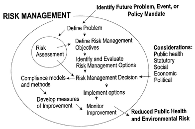

Fig. 1 Scientific and technical contributions to risk management.

In the area of environmental analysis, improvements in analytical instrument technology have reduced the scale of many previously insurmountable problems in environmental analysis, such as the analysis of small concentrations of contaminants in water. Yet, many challenges remain. These are largely tied to the properties of the analyte that make it difficult to study, or to the presence of substances within the sample that interfere with the study of the target analyte specifically. Sometimes these problems are confounded by the need to determine a contaminant at trace levels or to accurately determine small changes in contaminant concentration. Given the current level of interest in environmental issues, many groups in government, academia and the private sector have developed analytical methods to support particular objectives. For example, regulation compliance monitoring techniques have been developed and rigorously tested in order that water testing laboratories can provide reliable data to help improve the quality of the drinking water. These methods are often optimized for particular analytes in finished drinking water, which is engineered to conform to established guidelines. However, for research purposes, it is often necessary to test waters and other sample matrices that do not conform to these strict guidelines. This can markedly complicate the situation and lower confidence in the results of these tests applied to research circumstances. Further difficulties arise when existing methods are not appropriate for a particular contaminant, or, more confoundingly, when a method does not work adequately for an analyte for which the method was designed. In the following sections, some difficulties in applying standard methodology to research problems will be discussed, together with some solutions used in our risk management, analytical chemistry laboratory. Other risk management laboratories face similar challenges. The research problems and analytical solutions cited are therefore by no means an exhaustive list of the research that supports risk management issues, but rather are designed to show solutions used in our laboratory to solve the problems encountered. The focus of this paper is a discussion of the analytical chemistry applied to these challenges.

2 Examples of analytical chemistry for risk management

2.1 Stable association complex electrospray mass spectrometry applied to disinfection byproducts and Contaminant Candidate List compounds

Practitioners of electrospray mass spectrometry are familiar with the formation of undesirable complexes observed in this technique.² These complexes are formed due to substances already present within the samples or by reactions in the electrospray source. Altering the experimental conditions can avoid the formation of these complexes, which may interfere with the analysis. It is possible, however, to put this normally troublesome complexation phenomenon to good use. By the appropriate selection of a complexation agent, a selective complex can be formed between the analyte and the agent, and the mass of the complex can be used for analysis. The overall process may be referred to as ‘stable association complex electrospray mass spectrometry’ (cESI-MS). Not only does this increase selectivity, but it can also reduce interferences by increasing the observed mass above the chemical noise. Chemical noise is in the low mass region containing interfering ions, which may be molecules in the sample or ions formed within the electrospray source. cESI-MS has been applied to several analytical problems encountered in our risk management analytical laboratory. cESI-MS experiments are performed in the flow injection mode, and all operating parameters are readily achievable with standard, unmodified instrumentation.

One application of cESI-MS involves haloacetic acids (HAAs), which are a regulated class of disinfection byproducts (DBPs). DBPs refer to the thousands of compounds formed as byproducts of the disinfection of source water with a chemical oxidant. The oxidant destroys or inactivates microorganisms, but at the same time reacts with substances in the water to produce potentially toxic chemicals. Some DBPs are regulated and/or are the subject of intense study. One class of regulated DBPs are the nine combinations of bromo- and chloroacetic acids, commonly referred to as haloacetic acids (HAA9). Five of these HAAs are regulated in drinking water. To fully understand the complexities of HAA formation and ultimately the effect of HAAs on public health, in the strictest sense, it is necessary to be able to study HAA9. HAA9 are conventionally analyzed by EPA Method 552.2,³ but this is matrix and operator skill dependent, especially at low µg L⁻¹ concentrations. In particular, the performance of the method for the brominated trihaloacetic acids is problematic, because the final step in EPA Method 552.2 is methylation, in order that gas chromatography-electron capture detection (GC-ECD) may be used. Decarboxylation of brominated trihaloacetic acids occurs under the acidic conditions used for methylation. Therefore, as an alternative to methylation-GC-ECD, cESI-MS can be used for detection, thus avoiding the derivatization step. The HAA9 are extracted from the water with an organic solvent; the complexing agent, tridecafluoroheptanoic acid (13F), is then added to the extract, which is directly injected into the ESI-MS.⁴Fig. 2 shows the complex between 13F and HAA, represented as a proton-bound dimer.⁵ Because of uncertainties about the nature of complex formation in cESI-MS, it should be emphasized that the representation as a proton-bound dimer is tentative.

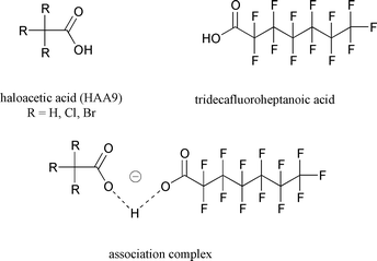Fig. 2 Structure of complexing agent, tridecafluoroheptanoic acid, and the analyte, HAA9, with R = H, Cl, Br. The complex is tentatively shown as the proton-bound dimer.

Fig. 3 shows five replicate injections of a 5.3 µg L⁻¹ standard. The inset mass spectrum shows the tribromoacetic acid complex. Sub-µg L⁻¹ detection limits for HAA9 (Table 1) and good comparability with EPA Method 552.2 are achieved for the non-decarboxylating analytes.⁴ In addition, several waters were studied with this technique, using all HAA9, and differences were noted between the proclivity of certain waters to form chlorinated HAAs and others to form brominated HAAs.

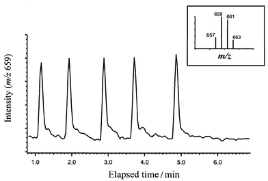Fig. 3 Flow injection peaks for haloacetic acid extractions. Each peak represents a separate 30 µL injection of an extract of a deionized water fortified with HAA9. The tribromoacetic acid concentration in the deionized water was 5.3 µg L⁻¹. The injection-to-injection error for the measured peak area from the five injections was 4%.

Table 1 Masses of the ions observed for HAA9 mixture in deionized water, method detection limits (MDLs), the amounts injected to determine the MDL and the largest concentration of each haloacetic acid investigated in this study

Haloacetic acid	Abbreviation	m/z observed	MDL^a/mg L^−1	LCI^b/mg L^−1
a Based on 3.14σn − 1 of n = 7. The concentrations used to determine the MDL were generally 3–6 times the MDL, depending on the concentration of the HAA in the mix. b LCI is the largest concentration investigated.
Chloro	MCA	457	0.60	48
Dichloro	DCA	491	0.32	48
Bromo	BAA	501	0.62	32
Trichloro	TCA	525	0.13	16
Bromochloro	BCA	535	0.26	32
Bromodichloro	BDCA	571	0.35	32
Dibromo	DBA	581	0.33	16
Dibromochloro	DBCA	615	0.64	32
Tribromo	TBA	659	0.45	16

---

In the midst of the cESI-MS study of HAA9, issues regarding the environmental impact of the perchlorate ion arose, and the applicability of cESI-MS to this analyte was investigated.⁶ Perchlorate is a powerful oxidizer, which may be released to the environment during the use and maintenance of rocket motors, and is also found naturally in some nitrate deposits. The solubility and mobility of perchlorate lends itself to groundwater contamination. When this contaminated water is used as a drinking water source, there are potential health effects associated with perchlorate. Namely, perchlorate can interfere with the proper functioning of the thyroid gland. Therefore, perchlorate was added to US EPA's Contaminant Candidate List (CCL), the list from which contaminants may be selected for future regulation.⁷ Perchlorate is also subject to the Unregulated Contaminants Monitoring Regulation (UCMR).⁸ Conventional analysis of perchlorate is based on high-performance liquid chromatography (HPLC) with conductivity detection, for instance by EPA Method 314.0.⁹ This type of detection is relatively non-specific and is subject to interferences, which obscure the study of perchlorate and may not withstand legal challenges.

cESI-MS was applied to perchlorate determination in drinking water, and detection limits of 100 ng L⁻¹ were achieved through selective extraction of perchlorate from drinking water as an ion pair with a cationic surfactant (quaternary ammonium salt).¹⁰ The sample work-up procedure involved extraction with a large volume of organic solvent, removal of the solvent and reconstitution in a different solvent. The cationic surfactants, mostly alkyltrimethyl salts, are used to ion pair aqueous perchlorate, forming extractable ion pairs. The cationic surfactant associates with the perchlorate to form a complex that is detectable by ESI-MS. The selectivity of the extraction and the mass spectrometric detection increases confidence in the identification of perchlorate.¹⁰Fig. 4 shows the ion pair and the association complex. The structure of the association complex is unknown with respect to the precise location of the second anion.

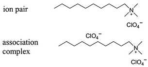Fig. 4 Drawing of the ion pair between perchlorate and the quaternary ammonium surfactant, and a tentative representation of the association complex observed in cESI-MS perchlorate analysis.

In our studies with larger numbers of samples, it was found to be advantageous to develop a different sample work-up in order to reduce the analysis time and minimize the generation of excess organic solvents as hazardous waste. For this purpose, we developed a microextraction procedure¹¹ which reduced the amount of sample needed from 500 mL to 38 mL with appropriate reductions in labor and solvent usage. Even though the nominal extractive preconcentration factor was about 25 times less in the microextraction, the detection limit was only about three times higher, at 300 ng L⁻¹. This unexpected result allows for the use of the small volume extractions described in the present study. The cause of this effect may be due to a change in the electrospray efficiency. As solutions become more ionic, the efficiency of the electrospray process typically drops. Thus, when the preconcentration factor is very large, the ionic strength increases as the surfactant concentration increases. A smaller concentration factor may therefore increase the analytical signal via a higher electrospray efficiency, which partially makes up for the loss in analyte concentration due to a lower amount of analyte preconcentration in the extraction step. The method detection limit (MDL) of the small volume extraction possibly may be lowered by careful study of the extraction ratio. However, at 300 ng L⁻¹, the MDL is sufficient to accomplish the primary goal of the cESI-MS experiment, namely to provide confirmation for ion chromatography used in US EPA Method 314.0,⁹ which has a detection limit of around 530 ng L⁻¹.

Fig. 5 shows a mass spectrum of 100 µg L⁻¹ perchlorate extracted from deionized water and observed with cESI-MS. The peak assignments are shown for the various trimethyldecylammonium (C10) complexes. Because C10 was used as a bromide salt, three complexes are detected: (i) the complex with C10 and two bromide ions; (ii) the complex with C10 and bromide and perchlorate; and (iii) the complex with C10 and two perchlorate ions. In practice, it is more reliable to quantify using the bromide–perchlorate–C10 complex rather than the perchlorate–perchlorate–C10 complex. The bromide–perchlorate–C10 complex produces a larger signal, probably due to the larger amount of bromide present from the use of the C10 bromide salt. The larger signal from the bromide–perchlorate–C10 complex may also reflect a greater tendency for this complex to form.

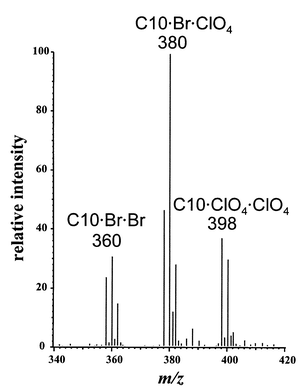Fig. 5 Mass spectrum of 100 µg L⁻¹ perchlorate in distilled water extract. The ions with which the trimethyldecylammonium (C10) cationic surfactant is complexed are indicated. The injection volume was 50 µL. The remainder of the m/z range contains noise.

For drinking water, the cESI-MS results compare well with ion chromatography, increasing confidence in both techniques.^10,11 After these investigations with drinking water, several sample matrices were investigated using cESI-MS, including bottled waters,¹² plant tissue¹³ and fertilizers.¹⁴ Sample preparation techniques vary among the media, but they all involve the following steps. First, an aqueous solution is prepared by a variety of means, depending on the media. Basically, plant tissue is pulverized in a blender and extracted with deionized water,¹³ whereas fertilizers are dissolved in deionized water.¹⁴ Then, as with the drinking water samples, the complexing agent is added to the aqueous solution, and the solution is extracted with an organic solvent.

Another example¹⁵ of the application of cESI-MS to a CCL compound is that of cyanuric acid, a suspected gastrointestinal or liver toxicant, which has gained interest as a potential degradation product of triazine herbicides, such as simazine and atrazine. The cyanuric acid is extracted from the water through a microscale liquid–liquid extraction prior to addition of the complexing agent, quaternary ammonium surfactants. This study¹⁵ provides insight into the mechanism of electrospray for the formation of these complexes, specifically with regard to the surface activity of the different surfactants and the chemistry of the surfactant–cyanuric acid complexes. The cESI-MS MDL for extraction of a 1 mL aqueous solution of cyanuric acid was 130 µg L⁻¹. The cyanuric acid concentrations determined with cESI-MS were not significantly different at the 95% confidence level to those determined by conventional HPLC. A recovery of 100% from a fortified urine sample illustrated the robustness of the technique.

2.2 Gas chromatography-mass spectrometry analysis of disinfection byproducts and Contaminant Candidate List compounds

Gas chromatography-mass spectrometry (GC-MS) is an instrumental technique often applied to environmental analysis because of its ability to provide both qualitative and quantitative data. Frequently, techniques developed for compliance monitoring or exposure studies are readily adaptable to risk management analytical needs for both routine analysis and research purposes. Sometimes, specialized GC-MS techniques are required, such as for the analysis of bromate, an ozonation DBP.¹⁶ A 22 ng L⁻¹ detection was achieved by conversion of bromate to a species amenable to negative ion GC-MS analysis.¹⁶ By contrast, ion chromatography analysis of bromate by EPA Method 300.1¹⁷ achieves a detection limit of around 2 µg L⁻¹. Another recent example is the analysis of a group of compounds on the CCL, namely the degradation products of triazine herbicides.¹⁸ The performance of water treatment studies for these compounds requires appropriate analytical methodology. In this case, there are no promulgated regulatory methods for two of these compounds, deethyl atrazine (DEA) and deisopropyl atrazine (DIA). Both of these compounds have been found, sometimes at significant concentrations, in source waters. In GC-MS analysis, DEA can coelute with DIA. The coelution of DEA and DIA can induce a significant (up to ∼50%) positive bias in the DEA determination when using an ion trap mass spectrometer as the detector.¹⁸ The DIA determination is unaffected by the coelution within experimental error. This may be explained in terms of gas phase ion fragment populations. Fig. 6 shows possible fragmentation pathways for DEA and DIA. Because DEA and DIA are structurally similar, the fragmentation of both DEA and DIA produces an ion with m/z 172 through different mechanisms. The presence of additional amounts of this common ion from DIA may shift the gas phase ion reaction towards m/z 187 for DEA, effectively enhancing its signal, corresponding to the experimental observation. By contrast, there is no common fragment with m/z 158 (a fragment ion of DIA). Thus, the signal from DIA is not affected, while DIA may enhance the DEA signal via the equivalent common ion. There are several strategies for quantifying DEA in the presence of DIA when using an ion trap mass spectrometer. One is to change the chromatography conditions, which may substantially increase the analysis time and decrease productivity. Another is to use a quadrupole rather than an ion trap mass spectrometer, if the equipment is available. A straightforward solution is to apply a correction factor to the observed DEA concentration. This correction factor can be calculated from the measured DIA concentration.¹⁸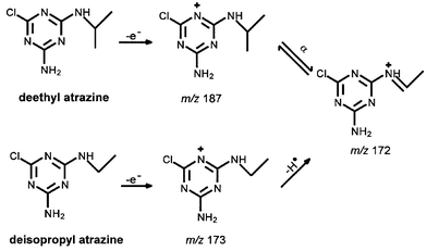

Fig. 6 Possible gas phase reaction pathways for deethyl atrazine (DEA) and deisopropyl atrazine (DIA).

2.3 Analysis of colloid/particle systems

Colloids and particles play a large role in many processes of interest to risk management.¹⁹ The characterization of these colloid/particle systems presents a number of technical challenges, mainly related to the small size of the particles/colloids (submicrometer to micrometer). To this end, several fractionation techniques have been investigated for research problems encountered in our laboratory. One, based on sedimentation field flow fractionation, was used to study iron(III) colloids formed in the presence of phosphate.²⁰ The fate and transport of metallic pollutants through a watershed are related to the characteristics of undissolved solid particles to which they are bound.²¹ Removal of these particles and their associated pollutants via engineered structures, such as settling ponds, is one goal of storm water management. Because the particles most often implicated in metal pollution have nominal diameters of <50 µm, split-flow thin cell (SPLITT) fractionation was investigated to study the metal loading as a function of the particle settling rate. Several diverse particle samples–soil, urban dust and parking deck sweepings–were fractionated using this technique, and the metal loadings were quantified with inductively coupled plasma-atomic emission spectrometry.²²Fig. 7 shows the experimental set-up for this type of experiment. The experiment is straightforward and performs reliably, reproducibly and rapidly. Fractionation of particles in the SPLITT technique occurs within the SPLITT cell, which is a thin (0.38 mm) channel with flow splitters centered in the channel on each end. As seen in Fig. 7, two flows (one containing the sample) enter the channel, and two flows exit. Under the influence of gravity, fractionation occurs as the particles, based on their settling rates, interact with the flow splitters and emerge from outlet a or outlet b.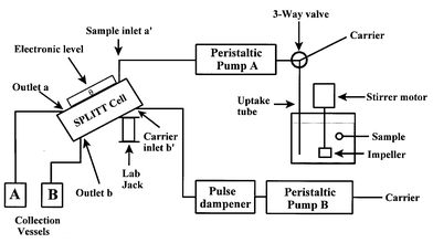

Fig. 7 Diagram of the experimental set-up for SPLITT fractionation.

Fig. 8 shows the results of a typical application of this technique to a soil sample, NIST 2710, and a dust sample, NIST 1649a.²² The dried samples were added at a concentration of 0.1% (w/w) to deionized water and were then passed through a 40 µm stainless steel screen to remove oversized particles. In interpreting these cumulative plots (Fig. 8), it is instructive to examine the top panel, constructed from data obtained for NIST 2710. In this material, ∼20% of copper is found on particles that have a relative settling diameter of <2 µm, ∼75% on particles <10 µm and nearly 95% on particles <18 µm. The variation of cumulative loading with relative settling diameter is similar for all the metals shown in the figure. This suggests that the particles in this sample have similar origins; perhaps they were formed by the physical breakdown of larger original particles.

Fig. 8 Results for SPLITT fractionation of NIST 2710 (soil) (top) and NIST 1649a (urban dust) (bottom). The metal loading is shown as a function of the relative diameter. The metal loading is expressed as the percentage of metal found on particles smaller than the associated relative diameter.

The data in Fig. 8 for the soil sample (NIST 2710) in the top panel contrast markedly with the data for the urban dust (NIST 1649a) in the bottom panel. In the bottom panel, the shapes of the cumulative metal loading versus settling diameter plots vary significantly among the metals. NIST 1649a appears to be composed of a mixture of particles from different origins, as might be expected for a dust sample. Alternatively, different metals may have different uptake behavior for different size fractions in the sample. Of particular interest is the unexpected result for NIST 1649a that, within experimental error, ∼100% of the zinc is found on particles with a relative diameter of <2 µm. This suggests that the zinc in NIST 1649a (Fig. 8, bottom) is not associated with particles that settle significantly enough to be fractionated. According to the supplier, NIST 1649a was collected in the St. Louis, MO, area. A zinc smelter is located within 30 miles of St. Louis. Thus, the zinc in NIST 1649a may originate from zinc oxide from airborne deposition. Plots like those in Fig. 8 could be useful in establishing settling pond operating conditions by supporting target pollutant removal decisions. For instance, if the target is the removal of 80% of the lead, the settling pond must be operated under flow conditions that will allow the removal of particles >2 µm, as predicted by Fig. 8 (top). In this example, Fig. 8 establishes that the remaining ∼20% of the lead is associated with very small particles (<2 µm) that may be difficult to remove by normal settling processes. Additionally, from Fig. 8 (bottom), it can be seen that, if zinc in the watershed is a problem, it would have to be removed by means other than simple settling, such as the addition of coagulants.

There are several advantages of using SPLITT fractionation to provide useful and accurate correlation between metal loadings and particle settlability.²² First, SPLITT fractionation is relatively rapid, taking <5 min per sample in these demonstrations, and the sampling time can be reduced if less resolution is acceptable. Second, small quantities (<0.5 g) of sample are required, which is important for samples where the amount of native material is limited. Third, SPLITT fractionation provides higher resolution than other techniques. The samples used for demonstration contain certain contaminants whose concentration varies rapidly over small changes in particle settlability. These changes would have been missed by other low resolution techniques, which could potentially affect settling pond management decisions. With regard to these decisions, the different particles presented illustrate the potential for SPLITT to characterize the type of particles/pollutants that are expected to enter a settling pond, which will contain a mixture of particles from different sources. By individually examining the contaminant sources–parking lots, soils, dusts, etc.–resources may be appropriately distributed to ensure that difficult to remove (and potentially dangerous) particles and their associated pollutants never reach the watershed.

2.4 Matrix-assisted laser desorption time of flight mass spectrometry characterization of Cryptosporidium parvum oocysts

Cryptosporidium parvum is an obligate protozoan parasite which causes cryptosporidiosis, a potentially fatal gastrointestinal illness.^23,24 Much environmental monitoring and risk management research has been directed at detecting and treating water contaminated with C. parvum, and this microorganism presents challenges at every turn. One challenge facing treatment research is the variability between oocysts produced from different sources.^25,26 Namely, the sources vary in their ability to be treated, particularly in their resistance to chemical disinfectants. Therefore, matrix-assisted laser desorption time of flight mass spectrometry (MALDI-ToF-MS) was investigated as a means to study the lot-to-lot variability of oocysts by our in-house facility.²⁷ MALDI-ToF-MS was used to investigate whole and freeze–thawed C. parvum oocysts. Whole oocysts revealed certain mass spectral features. Reproducible patterns of spectral markers and increased sensitivity were obtained after oocysts were lysed with a freeze–thaw procedure.²⁷ A mass spectral ‘fingerprint’ of C. parvum was calculated from about 25 peaks in the mass spectrum of the freeze–thawed oocysts, and is shown in Fig. 9. Spectral marker patterns for C. parvum were distinguishable from those obtained for C. muris. One spectral marker appears specific for the genus, while others appear specific at the species level. Three different C. parvum lots were investigated, and similar spectral markers were observed in each. Disinfection of the oocysts reduced and/or eliminated the patterns of spectral markers.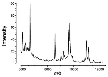

Fig. 9 MALDI-ToF-MS of freeze–thawed C. parvum oocysts.

The mass spectral ‘fingerprint’ of C. parvum calculated from about 25 peaks in the mass spectrum of the freeze–thawed oocysts (Fig. 9) represents approximately 70 000 oocysts, i.e. less than 0.5% of the total oocysts per production batch.²⁷ The elements of the fingerprint are defined by F = {l_i,s_li,p_i} where, for each peak i, l_i is the average peak location, s_li is the standard deviation in the peak location and p_i is the fraction of replicates in which peak i appears. The fingerprint may be represented, for instance, by the data in Table 2. In Table 2 (5 month column), most of the peaks appear in each lot and have p_i = 1. Two listed have p_i = 0.67; in these cases, the peak was visually present, but its mass could not be confidently determined. The set of peaks between 6796 and 7950 only appeared in one lot, so p_i = 0.33. Also included in Table 2 is the standard deviation in l_i. Larger values of the standard deviation in l_i are associated with difficulties in mass assignment for broader and/or smaller peaks. Thus, the peaks with p_i = 0.33 tend to be broader and/or smaller.

Table 2 Fingerprint parameters calculated from three lots of C. parvum

5 months			11 months
li(m/z)	sli(m/z)	pi	li(m/z)	sli(m/z)	p i
6040	5	1	6048	15	1
6251	2	1	6251	2	0.75
6285	5	1	6285	5	0.75
6398	6	1	6398	6	0.75
6637	6	1	6642	10	1
6796	14	0.33	6791	14	0.25
7220	15	0.33	7205	15	0.25
7567	11	0.33	7554	11	0.25
7739	8	0.33	7732	8	0.25
7950	12	0.33	7938	12	0.25
8579	10	1	8595	31	1
8821	5	1	8828	15	1
9036	6	1	9041	10	1
9118	5	1	9127	18	1
9178	4	0.67	9159	33	0.75
9243	9	1	9251	16	1
9327	3	1	9335	15	1
9645	2	1	9653	16	1
9724	4	1	9732	15	1
10755	3	1	10659	15	1
10910	6	1	10763	16	1
11024	7	1	10920	20	1
11192	13	0.67	11032	17	1
12072	8	1	11199	15	0.75

---

Using the proposed fingerprint of C. parvum contained in Table 2, comparison of future lots can be made through the use of the tabulated parameters. This fingerprint may be useful for quality control comparison with subsequent lots from in-house production, i.e. if a future lot produces a fingerprint that differs markedly from that in Table 2, action may be warranted. In considering an action level for quality control, if an arbitrary 50% (based on reported bacterial fingerprints) of the peaks are present, then the organism is confidently identified. In Table 2 (5 month column), >70% of the peaks are found in all C. parvum lots. Therefore, if the calculated fingerprint parameters of an unknown C. parvum lot match an arbitrary ∼70% of the parameters in Table 2, confidence in the lot's production quality may be increased.

Changes in the fingerprint with time are revealed in Table 2 by comparing the 5 month and the 11 month columns.²⁸ The values for the average peak location (l_i) change, but these changes are not greater than experimental error (s_li). The change in the fingerprint is revealed through a change in p_i for a peak. Some values for p_i increase with increasing time, which results from some peaks being absent in the mass spectrum recorded at the earlier aging time. A peak with p_i = 1 at all times has not changed. The more interesting case is when peaks are absent, indicated by decreases in p_i, e.g. from p_i = 1 to p_i = 0.75. Table 2 shows that 14 peaks (p_i = 1) appear in the spectra acquired from oocysts at both periods of aging. By contrast, four peaks are no longer observed at 11 months. The peaks that are missing are m/z 6251, 6285, 6398 and 12072. Fig. 9 shows that these peaks exhibit less intensity than those that are present, particularly for m/z 12072. However, m/z 6251, 6285 and 6398 may belong to a ‘family’ of peaks between m/z 6000 and 7000. C. parvum is known to have families of related biomolecules, i.e. the well-known 17 kDa C. parvum antigen is actually ten proteins between 14 kDa and 17 kDa. Further exploration of these three peaks and their relationship to C. parvum activity is warranted.

3 Conclusions

The examples described in this paper provide glimpses into the many complex challenges facing analytical chemistry for risk management research. Some examples provide high quality data for analytes that are not amenable to other methods. In other cases, they significantly complement and increase confidence in the quality of data obtained by other techniques. Better data may allow for better risk management decisions. For example, cESI-MS allows the accurate quantification of HAA9, which is important to risk management in providing data suitable for studying the formation and fate of HAA9. Present methods measure HAA5 well, but without data for all HAA9, it is difficult to obtain a complete picture, i.e. an accurate mass balance. The analysis of perchlorate and cyanuric acid by cESI-MS allows mass-based identification and quantification, with confidence unrivaled by conventional methods. The GC-MS experiments contribute to the accurate quantification of the respective analytes, which is needed to provide good quality data for CCL compounds. In this manner, risks may be properly assessed, and the proper chemicals may be regulated in the future. The SPLITT fractionation may impact on storm water settling pond management decisions, again by providing high quality data. The C. parvum technique presented impacts on the quality of risk management research in the area of the treatment of this important microorganism, by potentially lowering the variability in oocyst disinfectability. It is this disinfectability that is an important variable in setting drinking water standards to reduce the risk from this microorganism. While it is tempting to set the standards conservatively, if this is unnecessary due to better understanding of the oocysts, substantial cost savings in treatment operations may be realized.

These techniques provide solutions to special research needs. Of course, some risk management research activities are of a more routine nature, and these continue to benefit from methods designed for compliance monitoring. However, as environmental challenges become increasingly complex, the complementary and synergistic nature of environmental monitoring and risk management analysis becomes more apparent and intriguing. For example, in the CCL regulatory framework, candidate contaminants are legally required to be amenable to analytical determination in finished water. Additionally, risk management drinking water treatment research is required for a candidate contaminant, and so the analytical methods developed should also keep in mind the necessities of treatment research, namely matrices far more complicated than finished drinking water. On another risk management research front, improvements in understanding water quality and its relationship to the aquatic ecosystem will demand analytical chemistry capable of dealing with the complexities of the watershed but still producing tractable data.

References

1. US EPA, Strategic Plan for the Office of Research and Development, EPA/600/R-96/059, US EPA, Cincinnati, OH, 1996, http://www.epa.gov/ORD/SP/documents/ord96strplan.pdf. See also http://www.epa.gov/ORD/SP/index.htm.
2. W. M. A. Niessen, Liquid Chromatography-Mass Spectrometry, Marcel Dekker, New York, 1999.
3. D. J. Munch, J. W. Munch and A. M. Pawlecki, Methods for the Determination of Organic Compounds, Supplement III, EPA 600/R-95/131, US EPA, Cincinnati, OH, 1995.
4. M. L. Magnuson and C. A. Kelty, Anal. Chem., 2000, 72, 2308.
5. O. Debré, W. L. Budde and X. Song, J. Am. Soc. Mass Spectrom., 2000, 11, 809.
6. E. T. Urbansky, M. L. Magnuson, D. Freeman and C. Jelks, J. Anal. At. Spectrom., 1999, 14, 1861.
7. US EPA, Fed. Reg., 1998, 63(40), 10274; see also US EPA, Drinking Water Contaminant List, EPA-815-F-98-002, US EPA, Cincinnati, OH, 1998.
8. US EPA, Fed. Reg., 1999, 64(180), 50555.
9. D. P. Hautman, D. J. Munch, A. D. Eaton and A. W. Haghani, US EPA Method 314.0. Download at: http://www.epa.gov/safewater/methods/met314.pdf.
10. M. L. Magnuson, E. T. Urbansky and C. A. Kelty, Anal. Chem., 2000, 72, 25.
11. M. L. Magnuson, E. T. Urbansky and C. A. Kelty, Talanta, 2000, 52, 285.
12. E. T. Urbansky, M. L. Magnuson, G. M. Brown and C. A. Kelty, J. Sci. Food Agric., 2000, 80, 1798.
13. E. T. Urbansky, M. L. Magnuson, C. A. Kelty and S. K. Brown, Sci. Tot. Environ., 2000, 256, 227.
14. E. T. Urbansky, S. K. Brown, M. L. Magnuson and C. A. Kelty, Environ. Pollut., 2001, 112, 299.
15. M. L. Magnuson, C. A. Kelty and R. Cantú, J. Am. Soc. Mass Spectrom., 2001, 12, 1085.
16. M. L. Magnuson, Anal. Chim. Acta, 1998, 377, 53.
17. J. D. Pfaff, D. P. Hautman and D. J. Munch, US EPA Method 300.1, Cincinnati, OH. Download at: http://www.epa.gov/safewater/methods/met300.pdf.
18. M. L. Magnuson, T. F. Speth and C. A. Kelty, J. Chromatogr., A, 2000, 868, 115.
19. R. J. Allan, Role of Particulate Matter in the Fate of Contaminants in Aquatic Systems, Inland Waters Directorate, National Water Research Institute, Canada Centre for Inland Waters, Burlington, Ont., 1986.
20. M. L. Magnuson, D. A. Lytle, C. M. Freitch and C. A. Kelty, Anal. Chem., 2001, 73, 4815–4820.
21. P. J. Coughtrey, M. H. Marin and M. H. Unsworth, Pollutant Transport and Fate in Ecosystems, Blackwell Scientific Publications, New York, 1987.
22. M. L. Magnuson, C. A. Kelty and K. C. Kelty, Anal. Chem., 2001, 73, 3492.
23. J. P. Dubey, C. A. Speer and R. Fayer, Cryptosporidiosis of Man and Animals, CRC Press, Boca Raton, FL, 1990.
24. R. Fayer, Cryptosporidium and Cryptosporidiosis, CRC Press, Boca Raton, FL, 1997.
25. J. H. Owens, R. J. Miltner, T. R. Slifko and J. B. Rose, presented at the Water Quality Technical Conference, October 31–November 3, 1999, Tampa, FL.
26. J. L. Rennecker, B. J. Marinas, J. H. Owens and E. W. Rice, Water Res., 1999, 33, 2481.
27. M. L. Magnuson, J. H. Owens and C. A. Kelty, Appl. Environ. Micro., 2000, 66, 4720.
28. M. L. Magnuson, J. H. Owens and C. A. Kelty, presented at the 49th American Society Conference on Mass Spectrometry and Allied Topics, May 27–31, 2001, Chicago, IL.

---

Footnote

† Use of trade names or specific manufacturer's equipment or supplies does not constitute endorsement by the US EPA.

---