Prediction of high pressure phases in the systems Li₃N, Na₃N, (Li,Na)₃N, Li₂S and Na₂S

Abstract

The prediction of high pressure phases of a chemical system is realized as a two-step process: identification of structure candidates through the global exploration of their energy landscapes over a range of different pressures, followed by a limited local optimization using ab initio methods. The application of this recipe is presented for several systems, Li₃N, Na₃N, Li_xNa_(6 − x)N₂ (x = 1,…,5), Li₂S and Na₂S. We find that at standard pressure, the optimal configurations for the binary end compositions of the alkali nitrides, Li₃N and Na₃N, exhibit the Li₃N and Li₃P structures, respectively. Among the ternary compounds, the compositions with x = 2 and x = 4 are preferred, the optimal structures being ternary variations of the Li₃N structure type. At moderately high pressures, phase transitions from Li₃N to Li₃Bi related structures are predicted for all ternary compounds, while Na₃N and Li₃N exhibit transitions from Li₃P to Li₃Bi and Li₃N via Li₃P to Li₃Bi, respectively. The analogous study of the landscapes of Li₂S and Na₂S shows that a sequence of phase transitions from the CaF₂ structure via the PbCl₂ structure to the Ni₂In structure is expected.

---

1. Introduction

One of the main issues in the field of solid state chemistry is the question: to what extent is it possible to predict which solid compounds are capable of existence in a given chemical system?^1,2 Clearly, one can often provide suggestions based on similar compounds in related systems. With the introduction of high-throughput methods, sometimes collectively called combinatorial chemistry,³ it has become possible to perform rather systematic explorations of chemical systems. However, this approach is only feasible if the new compounds one aims for are easily accessible via a fast massively parallel application of traditional solid state chemistry synthesis techniques.

In most cases, however, synthesizing a new compound is a very challenging task, with even successful syntheses involving many careful experiments. Thus a priori information, whether a given chemical system admits the existence of stable or metastable compounds, would be very helpful. An important related issue is the question of whether one should expect phase transitions to occur, e.g. due to the application of high pressures or temperatures. Finally, there is the need to determine phase diagrams for ternary or higher compounds. While commonly a few compounds at certain compositions are already known in a given chemical system, there remain large unexplored regions in many phase diagrams.

An obvious alternative to the experimental exploration of a chemical system is the use of theoretical methods, in particular since high-speed computers and more or less robust programs^4–6 for ab initio quantum mechanical calculations have become available. Thus, over the past two decades, there have been a number of examples^7,8 where a hypothetical compound has been studied by first choosing a few possible structures by analogy to related systems, then calculating their energies using ab initio programs, and finally comparing the results. Depending on the amount of computer time available, the ab initio calculations have also involved some adjustments of the cell constants, yielding an equilibrium volume in the process.

While being very attractive at first sight, this approach still possesses several drawbacks. Most importantly, when guessing the possible structures, one must rely either on one's imagination or on the expectation that nature will repeat itself. Furthermore, these ab initio calculations are usually only feasible in the static limit, i.e. at T = 0 K excluding the zero point vibrations; using ab initio molecular dynamics at non-zero temperatures is very expensive computationally. Even a local optimization (in the static limit) of both the cell constants and the atomic coordinates is often quite difficult. Thus, in most instances, already estimates of the stability of the hypothetical compounds for non-zero temperatures are not possible, and high-temperature modifications that are not even metastable at low temperatures (i.e. that are not associated with a local minimum of the potential energy) are essentially inaccessible.

In order to address these problems, at least to a certain extent, we have developed a multi-stage approach to the prediction of structures of hypothetical compounds.¹ In a first step, a simple empirical potential is employed to approximately model the energy landscape of the chemical system of interest. Next, this energy landscape is explored for a fixed chemical composition using global optimization techniques and related search algorithms. This yields a large set of local minima of the system, each corresponding to a different structure candidate, together with estimates of the energetic and entropic barriers stabilizing these structures. In a further step, these minima serve as input to ab initio calculations, where a numerical local optimization of the cell is performed, as far as feasible. Finally, the whole procedure is repeated for many different compositions of the chemical system.

In this paper, we concentrate on the changes of the energy landscape as a function of pressure using lithium nitride as the main example. The results are combined with earlier studies^9,10 of the energy landscapes of alkali metal nitrides in the Li/Na/N system at zero pressure to yield an overview of their stable and metastable compounds as a function of pressure. Finally, results of an analogous study of the landscapes of Li₂S and Na₂S are presented.

2. Methods

2.1. Modeling the landscape

In general, many hundreds of global optimization runs have to be performed, in order to find the most important local minima of the energy landscapes of the systems under investigation. Since each run requires several hundred thousand or millions of energy evaluations, it is not possible to employ ab initio methods or elaborate computationally intensive potentials at this stage of the procedure. Thus, we model the systems as spherical ions that interact via empirical two-body potentials V_ij(r_ij), which only depend on the distances between the ions, r_ij. The expression for the enthalpy isThe potential V_ij(r_ij) consist of three terms: a (screened) Coulomb term for the electrostatic interactions among the ions, a repulsive r⁻¹² term, preventing the overlap of the ions, and an attractive r⁻⁶ term that represents the dispersive interactions:The parameters entering the empirical potential are the sum of the ionic radii multiplied by a scaling factor r_s, σ_ij = r_s(r_ion(i) + r_ion(j)), the parameters ε_ij, and the convergence parameter μ. Note that instead of a convergence factor one often employs an Ewald summation in order to compute the electrostatic energy^1,11,12 during the global optimization stage. However, we are predominantly interested in the possible structures and not so much in their actual energies, the latter being computed with ab initio methods in a second step. Since our experience shows that using a convergence parameter does not result in different major structure candidates, we have chosen this approach for the purpose of these calculations. Since the effective radius and the strength of the repulsive interaction can vary with pressure or local environment of the ions, it has turned out to be useful^10,12,13 to check the robustness of the local minima found by repeating the global optimizations for slightly different values of ε_ij, r_s and μ. In order to achieve a consistent picture in the study presented here, the variation of the landscapes as a function of pressure was performed for fixed parameter values, ε_ij = ε = 0.3, r_s = 1.1, and μ = 0.15, which had proven to be suitable in earlier studies‡ at zero pressure.¹⁰ The ionic radii employed during the optimization were r_ion (Li⁺) = 0.78 Å, r_ion(N³⁻) = 1.4 Å, r_ion(Na⁺) = 0.98 Å, and r_ion(S²⁻) = 1.94 Å. For the charges q of the ions, the formal charges were used, q(Li⁺) = +1, q(Na⁺) = +1, q(S²⁻) = −2 and q(N³⁻) = −3.

Since we are interested in crystalline compounds, we have applied periodic boundary conditions. Furthermore, the optimizations were performed for simulation cells that contain either two or four formula units of the respective compounds.

The calculations were repeated for a number of pressures, whose contribution to the enthalpy at T = 0 K is given in eqn. (1). Since only a limited number of global optimizations was feasible, we decided to start with a pressure of about one atmosphere, and increase the pressure subsequently by a factor of 10 each time. The reason for this choice of sample pressure was the expectation that at high pressures packing effects would dominate the possible structures, which are controlled by the repulsive terms in the interaction potential (cf.eqn. (2)). Thus changes in the landscape between subsequent “high” values of pressure should occur at considerably larger absolute pressure differences than those at “low” pressure values. Of course, in this way one will not be able to calculate e.g. a transition pressure. But at this stage, the goal is only to find structure candidates. No quantitative predictions of phase transitions or ground state energies etc. are attempted—the potentials used during the global optimization stage clearly lack the necessary accuracy. Instead, such predictions are based on the subsequent ab initio calculations.

2.2. Optimization procedure

The global optimizations were performed using the so-called simulated annealing algorithm,^14,15 which is based on random walks on the energy landscapes. Each step from configuration x_i to a neighbor x_i + 1 is accepted according to the Metropolis criterion, i.e. with probability min(1,exp(−(E_i+1 − E_i)/C). Here C is a control parameter, which is reduced to zero, according to a so-called annealing schedule. For a schedule we used C(n) = C₀fⁿ, n = 0,…,n_max. Typical values were C₀ = 1.3 eV atom⁻¹, f = 0.99, and n_max = 1000, with 300–1000 (depending on the system size) attempted random walk steps between adjustments of C. Typically, the move class (=rule according to which neighboring configurations are chosen at random) was: 80% movements of individual ions, 5% exchanges of ions, and 15% variations of the simulation cell.

One should note that the structure candidates obtained in this way are always slightly distorted from the true structure that usually exhibits at least some symmetry, i.e. they are given in the space group P1. We have determined the higher symmetry of the true structure using the symmetry finding and space group detecting programs SFND¹⁶ and RGS,¹⁷ respectively.§ The procedure yields idealized structures, which can then be used as input for the cell optimization when performing ab initio calculations. Of course, one would prefer to skip this idealization step by performing a full local optimization on an ab initio level, including the positions of the individual atoms in addition to the cell parameters. However, even now, such a full optimization is still a very difficult and time-consuming task. Thus, we have optimized only some of the cell parameters of the structure candidates, while keeping the symmetry of the structure and the relative atomic positions fixed.

Of course, even for the same structure, the cell constants and the exact locations of the atoms within the cell vary slightly from run to run, and both depend on pressure. Such variations have commonly been observed during all previous investigations of crystalline systems.^10,12,13 In order to deal with this aspect of global optimization on energy landscapes, we have introduced the concept of a “minimum basin”.¹⁸ Such a basin contains all nearly identical local minima that are associated with minute variations of a given structure candidate. These side minima possess tiny energetic barriers and are stabilized by boundary effects due to the long range Coulomb interactions.¶

Furthermore, it is commonly found that several of the structures belonging to distinct minimum basins are nevertheless very closely related in a topological sense.^10,12,13 Their coordination polyhedra and bonding topology are identical, and the configurations can be transformed into each other by very minor changes of the cell parameters together with slight displacements of the atoms. Thus, the structure candidates can be classified according to their topologically different structure types. In most but not all instances, it is obvious which of the several structures associated with the same structure type constitute the best minimum and should be chosen as the representative for the ab initio calculations.

2.3. Ab initio calculations

After performing some preliminary calculations using several ab initio methods, the Hartree–Fock method as implemented in the program CRYSTAL95⁴ was chosen for the calculation of the alkali nitrides. The test calculations showed⁹ both relatively fast convergence and good agreement with experimental values for the cell constants of Li₃N—the only system known in the alkali metal nitrides so far.^19–21 Basis sets were taken from the literature.^22,23 Similarly, for Li₂S and Na₂S, we again used CRYSTAL95, employing basis sets given in the literature,^24,25 where polarization d functions were included for Na and S.

In each system, we calculated the energy as a function of volume for a selected group of structure candidates, varying the volume by ca. 1% at each step. During the limited numerical local optimizations involved, the relative positions of the atoms and the symmetry of the structures were kept fixed. Furthermore, for orthorhombic or monoclinic structures, the ratios of the side lengths of the cells were usually not varied, i.e. only the total volume was changed during the optimization. The curve E(V) was then found by interpolation, where we have used the standard Murnaghan formula²⁶

Here, the four fit parameters B₀, B′₀, V₀ and C are the bulk modulus and its derivative, the equilibrium volume, and the zero of the energy scale, respectively.

We note that the slope of the E(V) curve for a given structure at some specified volume V′ equals the negative value of precisely that pressure p′ = −∂E/∂V, at which V′ corresponds to the equilibrium volume of the structure at the pressure p′. As a consequence, the enthalpy H(p) = E(V(p)) + pV(p) is given by the intercept of this tangent with the y-axis. Since a pressure-induced phase transition between two structures 1 and 2 implies that both the enthalpies and the pressures are equal in the two phases, H₁ = H₂ and p₁ = p₂ = p_c, the transition pressure is given by the negative slope of the common tangent of the E(V) curves, E_1,2(V), belonging to the two structures. Typically, the error in the computed value of the transition pressure is estimated to be roughly about 20–25%, where three possible sources of error dominate: limitations of the ab initio calculations (neglect of correlation energy, choice of basis sets), use of restricted local optimizations when computing data points, and the dependence of the fit of E(V) on the range and density of these data points. If no common tangent exists, or if the tangent implies negative transition pressures, one of the two structures will be metastable at all pressures. One should note, however, that these calculations only apply to zero temperature. It can very well be that for high temperatures, T ≫ 0, a plot of the respective free energies F_1,2(T;V) = E_1,2(T;V) − TS_1,2(T;V) instead of E_1,2(T = 0;V) would show a reverse order of the two structures regarding their thermodynamic stability.

3. Results

3.1. Li₃N

3.1.1. Global optimizations at different pressures. Global optimizations in the Li₃N system were performed for nine different pressures: p = 0 Pa, 0.16 MPa 1.6 MPa, 16 MPa, 160 MPa, 1.6 GPa, 16 GPa, 160 GPa and 1.6 TPa (0.1 MPa = 1 atm), with 80 simulated annealing runs for each pressure. A certain fraction of the runs did not end up in stable well-defined local minima but ended in amorphous or poorly condensed structures, in particular for “low” pressures, p ≤ 1.6 GPa. In the subsequent analysis, these runs have been discarded from the statistics. Overall, 42 different structures were found, which could be classified into 23 topologically different structure types.

For each pressure, about the same number of topologically different structure types was found during the global optimizations (7–10). However, for “low” pressures (p ≤ 1.6 GPa), the number of different local minima determined was considerably larger than for “high” pressures (p ≥ 16 GPa): 11–17 vs. 7–10, respectively (cf.Table 1). Quite generally, p = 16 GPa appears to constitute a “watershed” regarding the types of structures observed. With only one exception (I-Na₃N), no structure type was observed both below and above p = 16 GPa.

Table 1 Number of different structure candidates/structure types that occurred for a given pressure in eV Å⁻³ (=[16 GPa] = [160 kbar]) on the energy landscapes of Li₃N, Li₂S and Na₂S. In parentheses, the percentages of optimization runs that ended in amorphous, very distorted or poorly condensed phases are listed

Pressure	Li3N	Li2S	Na2S
0	15/8 (22%)	4/3 (10%)	5/5 (10%)
0.00001	16/9 (32%)	7/6 (15%)	8/6 (15%)
0.0001	14/7 (26%)	4/3 (20%)	10/7 (15%)
0.001	16/9 (8%)	5/4 (30%)	7/6 (25%)
0.01	17/10 (4%)	6/5 (25%)	9/8 (35%)
0.1	11/8 (6%)	6/4 (50%)	2/2 (5%)
1	10/7 (0%)	3/3 (10%)	2/2 (0%)
10	10/8 (0%)	2/2 (10%)	3/3 (30%)
100	8/7 (0%)	No runs	No runs

---

For all pressures, each of the structures exhibited a variation in the enthalpy on the order of 1% from one optimization run to the next. On the other hand, the variability of the unit cell volume for a given structure was much larger at “low” pressures than at “high” pressures (2% vs. 0.01%). This difference in variability was also present when an average over all minima observed at a given pressure was performed: both the average volume and the standard deviation decreased with pressure. The reason for the large spread at “low” pressures is connected to a similarly large spread in coordination number of N by Li, of course (cf.Table 2). For “low” pressures, the structure candidates exhibited local coordination ranging from CN = 8 or 6 to CN = 14, with no well-defined structures occurring with CN = 9 or 10, however. On the other hand, for “high” pressures the coordination varied much less, CN = 12–15. In addition, the fraction of successful optimizations that reached the two most commonly found minimum basins (not always the ones with the lowest energy!) was very high, 65–90%, to be compared with 30–50% at “low” pressures.

Table 2 Average coordination numbers CN and their spread (in parentheses) for a given pressure in eV Å⁻³ (=[16 GPa] = [160 kbar]) on the energy landscapes of Li₃N, Li₂S and Na₂S

Pressure	Li3N	Li2S	Na2S
0	11.46 (6–14)	8.00 (8–8)	8.33 (8–10)
0.00001	11.40 (6–14)	8.07 (8–9)	8.20 (8–9)
0.0001	11.91 (8–14)	8 (8–8)	8.35 (8–10)
0.001	11.75 (8–14)	8.07 (8–9)	8.40 (8–10)
0.01	11.60 (8–14)	8.07 (8–9)	8.70 (8–11)
0.1	12.16 (11–14)	10.00 (8–11)	11.75 (11–12)
1	12.99 (12–15)	11.70 (10–12)	12.00 (12–12)
10	13.84 (12–15)	12.00 (12–12)	12.00 (12–12)
100	13.65 (12–15)	No runs	No runs

---

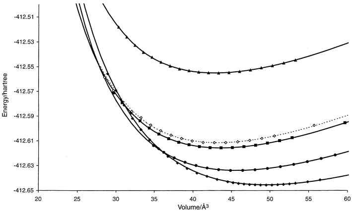
An important observation is the fact that for the landscapes at “low” pressure many local minima with rather high energies were found, in agreement with earlier results¹⁰ of global optimizations at p = 0 Pa. This suggests that a) the energetic and entropic barriers separating these minima from the rest of the landscape are quite substantial, and b) that the local densities of states in those high lying minimum basins are large enough to compete successfully with the energetically favored low energy minima.|| In this context, we note that there exists a large low energy region of the landscape at “low” pressures, where over 80% of all the successful optimization runs ended up. All the structure types belonging to this region can be derived from the Li₃Bi structure type by moderately large rearrangements of the ions, changing the coordination from 8 + 6 to 11 + 3, 12 + 2 or 13 + 1. Threshold investigations show that these minima are separated by rather small energy barriers that are crossed very quickly, indicating only small entropic contributions to the barriers. Furthermore, their E(V) curves when calculated on an ab initio basis are practically identical near the minimum of E(V) (cf.Fig. 1). In contrast, all other structure types that occur at “low” pressures appear to be separated by relatively large barriers from the remainder of the landscape. Data for selected structure types are found in the appendix.

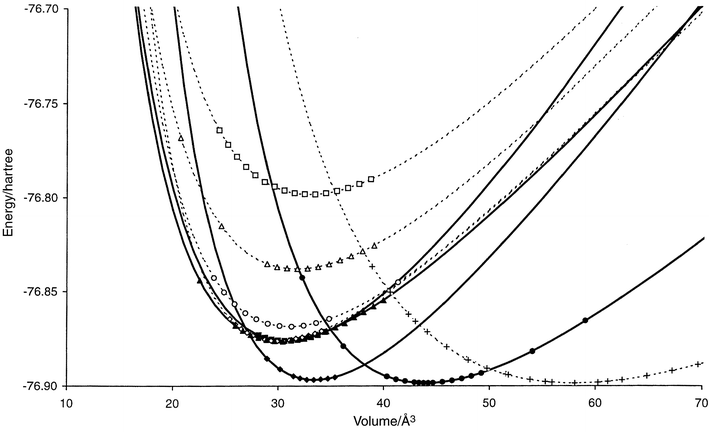Fig. 1 E(V) curves for promising structure candidates (cf.Table A1 in the appendix) in the system Li₃N. Li₃N: filled circles (solid), Li₃P: filled diamonds (solid), ReO₃: crosses (dashed), Li₃Bi: filled triangles (solid), I-Na₃N: filled squares (solid), Al₃Ti: hollow diamonds (dashed), Cr₃Si: hollow circles (dashed), AuCu₃: hollow squares (dashed), A1-Li₃N: hollow triangles (dashed). The computed data points used for the Murnaghan fit are shown for each curve. Structures that are found to be stable in some pressure range are shown as solid curves, while the metastable ones are given as dashed lines.

3.1.2 Ab initio calculations. For the most promising structure types, E(V) curves were computed, and are shown in Fig. 1. Analyzing these curves, it is found that several phase transitions are feasible for the Li₃N system. At p_c = 0.4 ± 0.1 GPa, a transition occurs from the Li₃N structure to the Li₃P structure, and at p_c = 27.6 ± 5.4 GPa a second transition from the Li₃P to the Li₃Bi structure. Finally, at extremely high pressures, p_c = 168 ± 35 GPa, a transition to I-Na₃N might take place. Furthermore, the ReO₃ structure appears to be metastable with a very small transition pressure, |p_c| < 0.1 GPa, relative to the Li₃N structure. These results confirm and extend earlier investigations,⁹ where only three of the structure types (Li₃N, Li₃P and Li₃Bi) found at p = 0 Pa had been taken into account.

3.2. Na₃N and (Li,Na)₃N

In earlier work, the energy landscape of Na₃N at zero pressure has been studied in detail.¹⁰ Quite generally, we note that many of the structure types observed for the Li₃N system reappeared for the landscape of Na₃N. Again many structure candidates related to the Li₃Bi structure were found. Using the threshold algorithm,²⁷ they were shown to be separated by only a small energy barrier (within the empirical potential model, of course). Thus, following the lead of the Li₃N system, E(V) curves were calculated only for the Li₃N, the Li₃P and the Li₃Bi structure types⁹ (cf.Fig. 2). It was found that the structure candidate with the lowest energy at zero pressure is the Li₃P structure, closely followed by the Li₃N structure. Since the equilibrium volume of the Li₃N structure is considerably larger than that of the Li₃P structure, it is no surprise that the only pressure induced phase transition found for this system was the one between the Li₃P and the Li₃Bi structure types at p_c = 13.8 ± 3.2 GPa. The Li₃N structure is metastable with a relatively small negative transition pressure, p_c = −0.3 ± 0.06 GPa, relative to the Li₃P structure.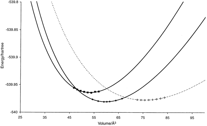

Fig. 2 E(V) curves for promising structure candidates (cf.Table A2 in the appendix) in the system Na₃N. Li₃N: hollow diamonds (dashed), Li₃P: filled diamonds (solid), Li₃Bi: filled squares (solid). The computed data points used for the Murnaghan fit are shown for each curve. Structures that are found to be stable in some pressure range are shown as solid curves, while the metastable ones are given as dashed lines.

Similarly, the energy landscape of the ternary system (Li_xNa_6 − xN₂) (x = 1,…,5) has been studied⁹ at zero pressure, and the results can be summarized as follows: At standard pressure, the compositions x = 2 and x = 4 are preferred, the optimal structures being ternary variations of the Li₃N structure type. Here, several of the possible placements of the cations on the Li positions in the Li₃N structure are found to lead to configurations that represent local minima of the energy landscape. In the optimal arrangements, the minority cations are located at the apices of the hexagonal bipyramids around the N ions, connecting the N containing layers. While ternary analogues of the Li₃Bi, I-Na₃N and Al₃Ti structure types are found as additional local minima, no analogues of the Li₃P, AuCu₃ or Cr₃Si structure types have been observed. Ab initio calculations show that at moderately high pressures, phase transitions from Li₃N to Li₃Bi related structures are predicted for all compositions x. However, the transition pressure is much higher (p_c = 7.8 ± 1.8 GPa, p_c = 7.2 ± 1.6 GPa) for the compositions x = 2 and 4, respectively, than for the compositions x = 1,3,5 (p_c = 0.3 ± 0.06 GPa, p_c = 2.9 ± 0.6 GPa and p_c = 1.6 ± 0.35 GPa, respectively). This serves as an indication that the preference for the compositions x = 2,4 should persist towards higher pressures. For comparison, the hypothetical transitions from the Li₃N to the Li₃Bi structure type for the binary end compositions, the Li₃N and the Na₃N system, would occur at p_c = 7.0 ± 1.5 GPa and p_c = 3.0 ± 0.6 GPa, respectively.

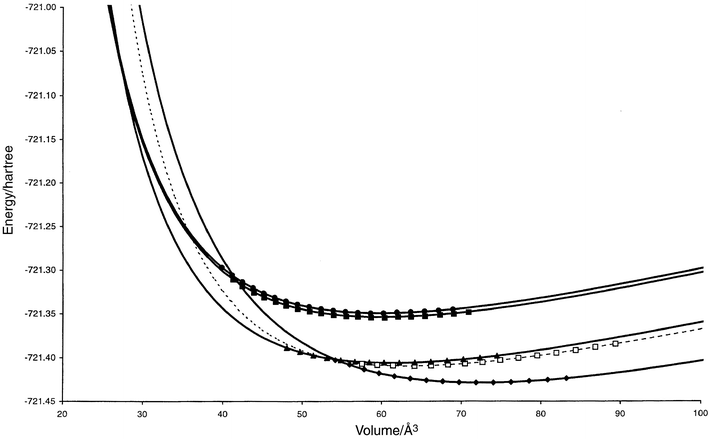
3.3. Li₂S and Na₂S

3.3.1. Global optimization runs for Li₂S and Na₂S at different pressures. For each of these related energy landscapes, 20 global optimizations were performed for pressures p = 0 Pa, 0.16 MPa, 1.6 MPa, 16 MPa, 160 MPa, 1.6 GPa, 16 GPa and 160 GPa each. For half of these runs, two formula units (Z = 2) per simulation cell were chosen, and for the other half four formula units (Z = 4). A total of 30 different structures were found, which could be classified in 17 structure types. Of these, 11 occurred in the Li₂S system (18 different local minima overall), and 16 in the Na₂S system (22 different minima overall), with the most important structure candidates present on both landscapes. In general, the same structure candidates were found both for landscapes with Z = 2 and for those with Z = 4, although a few structures that are based on primitive unit cells containing four formula units were only found in the latter case, of course. The additional freedom in the rearrangements of the atoms in the larger systems was also reflected in slightly smaller (ΔV < 1%) average volumes and slightly lower average enthalpies of the minimum structures for Z = 4 compared with Z = 2. Overall, well-defined structures occurred for all coordination numbers between 8 and 12. This differs from the Li₃N system, where no well-defined structures with CN = 9, 10 were found. Furthermore, both the spread of coordination numbers (cf.Table 2) and the spread in volumes of the structure candidates for a given pressure were considerably smaller than for Li₃N. Again, a distinct change in the types of structures that corresponded to local minima of the landscape occurred above a certain pressure, p = 160 MPa. Data for selected structure candidates are given in the appendix.

3.3.2 Ab initio calculations for Li₂S and Na₂S. As for the Li₃N system, the most promising structure candidates found for Li₂S were chosen for refinement optimizations. The corresponding E(V) curves are shown in Fig. 3. We see that for Li₂S a phase transition should occur at a pressure of about p_c = 24 ± 6 GPa from the CaF₂ (CN = 8) to the PbCl₂ structure (CN = 9), followed by another from the PbCl₂ to the Ni₂In structure (CN = 11) at p_c = 42 ± 9 GPa. Several high pressure structure candidates with even higher coordination numbers like the A1-Li₂S structure (hexagonal Na₁₂S prisms, space group P6/mmm) have also been investigated, but so far it appears that no further transition should occur up to 1 TPa.

Fig. 3 E(V) curves for promising structure candidates (cf.Table A3 in the appendix) in the system Li₂S. CaF₂: filled diamonds (solid), PbCl₂: filled circles (solid), Ni₂In: hollow diamonds (dashed), Ni₂In-(d) (see Discussion): filled squares (solid), A1-Li₂S: filled triangles (solid). The computed data points used for the Murnaghan fit are shown for each curve. Structures that are found to be stable in some pressure range are shown as solid curves, while the metastable ones are given as dashed lines.

Similar to the Li₂S system, we have also performed ab initio local optimizations for Na₂S. The results available so far indicate that a phase transition should occur between the CaF₂ and the Ni₂In structure, with a possible appearance of the PbCl₂ structure over a short intermediate pressure range. This might be followed by a transition to a 12-fold coordinated structure A1-Na₂S (space group I4₁/amd) at very high pressures. The transition pressure(s) for the transition(s) up to the Ni₂In structure are expected to lie in a pressure range around p_c = 11 ± 2.5 GPa, while either the A1-Na₂S structure or the A2-Na₂S structure might be stable above a pressure of p_c = 120 GPa.

4. Discussion

Perhaps the most striking result of the landscape investigations is the persistence of major features of the energy landscape when varying the pressure. Many of the important structure types correspond to deep-lying local minima over a wide pressure range, for both alkali metal nitrides and sulfides. The second general observation is the division of the structures into two groups, constituting local minima at either “high” or “low” pressures. This is no great surprise, of course, but it underlines the importance of exploring the energy landscape of a system at many different pressures.

When comparing the landscapes for different systems, it appears somewhat surprising that considerably more structure candidates are found for Li₃N than for Li₂S and Na₂S taken together. However, this might well be caused by the larger sample of optimization runs for the Li₃N system. Clearly, further optimizations are needed for the sulfides, which might result in a change in the number of distinct structures observed.

As was mentioned earlier, Li₃N is the only binary or ternary alkali metal nitride known so far. Its high pressure behavior has been studied in recent years, and the transition to the Li₃P structure we have found has been observed at ca. 0.6 GPa²⁸ by experiment. Taking into account experimental and theoretical uncertainties, this agrees well with the value of 0.4 GPa we have computed. Furthermore, there are hints at a transition to a high-symmetry structure like e.g. Li₃Bi somewhere in the pressure range from 10 to 35 GPa.^28,29 Again, this agrees well with our prediction of a transition to Li₃Bi or a closely related structure at p_c = 28 GPa. Clearly, more careful experimental investigations are needed to resolve the discrepancy between the experiments and allow a comparison with our calculations. We also note that our results are of the same order of magnitude as those of a recent LDA-based calculation²⁹ for Li₃N, where a transition pressure of 38 GPa has been suggested between the Li₃P structure (which was computed to be the equilibrium structure at standard pressure, however!) and the Li₃Bi structure.

Regarding Na₃N and the ternary system (Li,Na)₃N, no synthesis has proven to be successful so far, in spite of some claims in the past.³⁰ Thus we can only judge the results by comparing with the most closely related structures. Here, the fact that the energy landscapes of Li₃N and Na₃N are very similar lends confidence to the prediction of Na₃N existing either in the Li₃N or the Li₃P structure at standard pressure. For the ternary system, we note that in particular the Li₃N related structures with minority cations at the apices of the hexagonal bipyramids lead to very well balanced structures for Li ∶ Na ratios of 1 ∶ 2 (x = 2) and 2 ∶ 1 (x = 4). As a consequence, we might find phase separation instead of perfect mixing in the (Li,Na)₃N system. The preference for the Li₃N related modifications at standard pressure agrees well with the existence of ternary systems^31–33 of the composition (Li,M)₃N (M = Cu, Ni, Co, Mn, Fe), all exhibiting a Li₃N related structure with minority cations between the layers containing N ions.

While this is very encouraging, one needs to recall that in general further phases might be present that do not show the desired composition (Li,Na)₃N. In particular, elementary (gaseous) nitrogen and (metallic) sodium together with Li₃N might form as an alternative to the desired compounds, e.g. Li₂NaN or LiNa₂N.

Turning to the sulfides, recent experimental work³⁴ on Li₂S has shown that the transition to the PbCl₂ structure type does take place at p_c = 12 GPa, while the predicted transition to the Ni₂In structure at higher pressure has not yet been observed. Regarding experiments on Na₂S, transitions from the CaF₂ structure via the PbCl₂ structure to the Ni₂In structure have recently been observed³⁵ at pressures of about 5 GPa, and somewhere between 8 and 20 GPa, respectively, while further transitions at higher pressures have not yet been found.

In this context one needs to address the question of systematic errors in the qualitative and quantitative prediction of transition pressures. Beyond the basic limitations of each ab initio method, we face the requirement of having to use the same basis set and/or effective interaction potential for all volumes, in order to achieve consistency and comparability of the E(V) curves. This can lead to various cut-off problems when computing data points far away from the minimum of the E(V) curve. This is especially critical when starting from structure candidates that were only observed at high pressures, since here the starting point of the local optimization can be far removed from the minimum of the E(V) curve. While this has not been a problem for the sulfides up to now, it has proven to be rather difficult to achieve convergent E(V) calculations for the structure candidates found at very high pressures (p ≥ 160 GPa) in the Li₃N system. Thus these data have been excluded from the E(V) diagram in Fig. 1. A further potential source of error is the dependence of the fit on the available computed data points, especially when attempting extrapolations towards low volumes. Tests for e.g. the sulfide systems have shown that the curvature of the fitted E(V) curve can exhibit non-negligible changes upon addition of further data points.

A second concern is the restriction of keeping symmetry and atomic positions fixed during the local optimizations with ab initio methods. As a consequence, the computations produce at best upper bounds on the true E(V) curves of the compound. This caveat applies in particular if the structure under investigation is not highly symmetric or contains many atoms in general positions (x,y,z). Since we are rarely able to optimize all cell parameters and the positions of the atoms at the same time, it is quite likely that in such a case the true E(V) curve will lie somewhat lower than the computed one, resulting e.g. in a lower transition pressure. Directly related to this is the fact that a numerical optimization by hand (CRYSTAL95 has no gradient available) will always lack the precision of a gradient based optimization. An instance where a full optimization might be advisable is the PbCl₂ related structure found in Li₂S and Na₂S, which possesses a relatively low symmetry and contains many atoms in general positions, and is similar in energy to the Ni₂In structure in Na₂S. Thus, the corresponding E(V) curves computed for Li₂S (Fig. 3) and Na₂S (Fig. 4) should only be considered as a first approximation as far as quantitative conclusions are concerned.

Fig. 4 E(V) curves for promising structure candidates (cf.Table A4 in the appendix) in the system Na₂S. CaF₂: filled diamonds (solid), PbCl₂: hollow squares (dashed), Ni₂In: filled triangles (solid), A1-Na₂S: filled circles (solid), A2-Na₂S: filled squares (solid). The computed data points used for the Murnaghan fit are shown for each curve. Structures that are found to be stable in some pressure range are shown as solid curves, while the metastable ones are given as dashed lines.

In order to investigate the possible errors due to an incomplete local optimization, we have computed additional E(V) data points, both for Li₂S and Na₂S in the Ni₂In and the PbCl₂ modifications each. We find for most modifications, except for the PbCl₂ structure in Li₂S, that the data points resulting from the less restricted local optimization lie clearly below the curve obtained from the one-parameter optimization. Furthermore, there appears to be a slight shift to somewhat larger equilibrium volumes at zero pressure. In addition, we also studied the effect of including five more data points at low volumes for the fluorite structure of Na₂S. We find that the curvature of the E(V) curve changes significantly, leading to a large change of the transition pressure from 16 GPa to about 11 GPa. In general one should note that the effect of the potential errors appears to be very specific for each system and modification. Furthermore, the changes in the E(V) curve have the greatest impact in the range of very small volumes and extremely high pressures (p > 10 GPa).

Finally, we note that it is quite possible that a slightly distorted structure candidate with somewhat lower symmetry might be energetically preferable within some pressure range. An example is the Ni₂In structure type in Li₂S, which occurred as a local minimum both as a fully symmetric and a slightly distorted structure, called Ni₂In and Ni₂In-(d), respectively. For both, the E(V) curves have been computed and are shown in Fig. 3. We note that in this instance, the distorted version appears slightly more favorable at low pressures, while at high pressures both curves are nearly identical.

5. Summary

We have shown how a two-step procedure consisting of an exploration of the energy landscapes of chemical systems at various pressures using global optimization techniques, followed by a local optimization with ab initio methods, leads to successful predictions of pressure induced phase transitions. For those chemical systems where a synthesis has already been successful (Li₃N, Li₂S, Na₂S), the results agree well with experimental observations. But there still remains a challenge to the experimentalist, as additional predicted structures in the Li₃N, Na₃N, (Li,Na)₃N, Li₂S and Na₂S systems still await their realization. Tables A1–A4:

Table A1 Structure candidates for Li₃N that were selected for ab initio calculations

Li3N Minimum	Space group (number), origin choice, crystal system	Lattice constants a, b, c/Å; α, β, γ/°	Atom (multiplicity, Wyckoff symbol), fractional coordinates
Li3N	P6/mmm (191), hexagonal	a = 3.612, c = 3.875	Li2 (2c)	1/3	2/3	0
		α = 90.00, β = 90.00, γ = 120.00	Li1 (1b)	0	0	1/2
			N (1a)	0	0	0
I-Na3N	Pmmn (59), orthorhombic	a = 3.523, b = 4.929, c = 3.523	Li1 (4e)	3/4	0.5	0.72
		α = 90.00, β = 90.00, γ = 90.00	Li2 (2b)	3/4	1/4	0.18
			N (2a)	3/4	3/4	0.78
Al3Ti	I4/mmm (139), tetragonal	a = 3.502, c = 4.877	Li1 (4d)	1/2	0	1/4
		α = 90.00, β = 90.00, γ = 90.00	Li2 (2b)	1/2	1/2	0
			N (2a)	0	0	0
Li3P	P63/mmc (194), origin choice 2, hexagonal	a = 3.509, c = 6.262	Li1 (4f)	1/3	2/3	0.58
		α = 90.00, β = 90.00, γ = 120.00	N (2c)	1/3	2/3	1/4
			Li2 (2b)	0	0	0
Li3Bi	Fm3̄m (225), cubic	a = 4.957	Li (8c)	1/4	1/4	1/4
		α = 90.00, β = 90.00, γ = 90.00	N (4b)	1/2	1/2	1/2
			Li (4a)	0	0	0
AuCu3	Pm3̄m (221), cubic	a = 3.223	Li (3c)	1/2	1/2	0
		α = 90.00, β = 90.00, γ = 90.00	N (1a)	0	0	0
Cr3Si	Pm3̄n (223), cubic	a = 3.967	Li (6c)	1/4	0	1/2
		α = 90.00, β = 90.00, γ = 120.00	N (2a)	0	0	0
ReO3	Pm3̄m (221), cubic	a = 4.334	Li (3d)	1/2	0	0
		α = 90.00, β = 90.00, γ = 90.00	N (1a)	0	0	0
A1-Li3N	Cmma (67), orthorhombic	a = 3.972, b = 5.956, c = 5.372	Li (8m)	0	0.10	0.64
		α = 90.00, β = 90.00, γ = 90.00	N (4g)	1/2	1/4	0.74
			Li (4a)	1/4	1/2	0

---

Table A2 Structure candidates for Na₃N that were selected for ab initio calculations

Na3N Minimum	Space group (number), origin choice, crystal system	Lattice constants a, b, c/Å; α, β, γ/°	Atom (multiplicity, Wyckoff symbol), fractional coordinates
Li3P	P63/mmc (194), origin choice 2, hexagonal	a = 4.257, c = 7.524	Li1 (4f)	1/3	2/3	0.58
		α = 90.00, β = 90.00, γ = 120.00	N (2c)	1/3	2/3	1/4
			Li2 (2b)	0	0	0
Li3N	P6/mmm (191), hexagonal	a = 4.365, c = 4.590	Li2 (2c)	1/3	2/3	0
		α = 90.00, β = 90.00, γ = 120.00	Li1 (1b)	0	0	1/2
			N (1a)	0	0	0
Li3Bi	Fm3̄m (225), cubic	a = 5.995	Li (8c)	1/4	1/4	1/4
		α = 90.00, β = 90.00, γ = 90.00	N (4b)	1/2	1/2	1/2
			Li (4a)	0	0	0

---

Table A3 Structure candidates for Li₂S that were selected for ab initio calculations

Li2S Minimum	Space group (number), origin choice, crystal system	Lattice constants a, b, c/Å; α, β, γ/°	Atom (multiplicity, Wyckoff symbol), fractional coordinates
CaF2	Fm3̄m (225), cubic	a = 5.5	Li (8c)	1/4	1/4	1/4
		α = 90.00, β = 90.00, γ = 90.00	S (4a)	0	0	0
Ni2In-(d) (distorted, see text)	Cmcm (63), orthorhombic	a = 4.065, b = 7.870, c = 5.458	Na1 (4c)	0	0.67	1/4
		α = 90.00, β = 90.00, γ = 120.00	S (4c)	1/2	0.85	1/4
			Na2 (4a)	0	0	1/2
Ni2In	P63/mmc (194), hexagonal	a = 4.350, c = 5.220	S (2d)	1/3	2/3	3/4
		α = 90.00, β = 90.00, γ = 120.00	Li1 (2c)	1/3	2/3	1/4
			Li2 (2a)	0	0	0
A1-Li2S	P6/mmm (191), hexagonal	a = 3.824, c = 3.635	Li (2d)	2/3	1/3	1/2
		α = 90.00, β = 90.00, γ = 120.00	S (1a)	0	0	0
PbCl2	Pnma (62), orthorhombic	a = 6.278, b = 3.828, c = 7.470	Li1 (4c)	0.97	3/4	0.67
		α = 90.00, β = 90.00, γ = 90.00	Li2 (4c)	0.64	1/4	0.57
			S (4c)	0.25	1/4	0.61

---

Table A4 Structure candidates for Na₂S that were selected for ab initio calculations

Na2S Minimum	Space group (number), origin choice, crystal system	Lattice constants a, b, c/Å; α, β, γ/°	Atom (multiplicity, Wyckoff symbol), fractional coordinates
CaF2	Fm3̄m (225), cubic	a = 6.600	Na (8c)	1/4	1/4	1/4
		α = 90.00, β = 90.00, γ = 90.00	S (4a)	0	0	0
Ni2In	P63/mmc (194), hexagonal	a = 4.915, c = 5.950	S (2d)	1/3	2/3	3/4
		α = 90.00, β = 90.00, γ = 120.00	Na1 (2c)	1/3	2/3	1/4
			Na2 (2a)	0	0	0
A1-Na2S	I41/amd (141), origin choice 2, tetragonal	a = 3.755, c = 13.202	Na (8e)	1/2	1/4	0.21
		α = 90.00, β = 90.00, γ = 90.00	S (4b)	0	1/4	7/8
A2-Na2S	P6/mmm (191), hexagonal	a = 3.816, c = 3.696	Na (2d)	2/3	1/3	1/2
		α = 90.00, β = 90.00, γ = 120.00	S (1a)	0	0	0
Pb2Cl	Pnma (62), orthorhombic	a = 6.278, b = 3.828, c = 7.470	Na1 (4c)	0.71	1/4	0.42
		α = 90.00, β = 90.00, γ = 90.00	Na2 (4c)	0.95	3/4	0.30
			S (4c)	0.27	3/4	0.89

---

Acknowledgements

We would like to thank G. Stollhoff, K. Syassen, A. Vegas, and R. Hundt for valuable discussions. This work has been partly funded by the DFG via the Sonderforschungsbereich 408.

References

1. (a) J. C. Schön and M. Jansen, Angew. Chem., 1996, 108, 1358; (b) J. C. Schön and M. Jansen, Angew. Chem., Int. Ed. Engl., 1996, 35, 4001.
2. M. L. Cohen, Science, 1986, 234, 549.
3. (a) B. Jandeleit, D. J. Schaefer, T. S. Powers, H. W. Turner and W. H. Weinberg, Angew. Chem., 1999, 111, 1648; (b) B. Jandeleit, D. J. Schaefer, T. S. Powers, H. W. Turner and W. H. Weinberg, Angew. Chem., Int. Ed., 1999, 38, 2494.
4. R. Dovesi, V. R. Saunders, C. Roetti, M. Causa, N. M. Harrison, R. Orlando and E. Apra, CRYSTAL95, University of Torino, 1996..
5. P. Blaha, K. Schwarz and J. Luitz, WIEN97, Vienna University of Technology, 1997..
6. R. Car and M. Parinello, Phys. Rev. Lett., 1985, 55, 2471.
7. A. Y. Liu and M. L. Cohen, Phys. Rev. B, 1990, 41, 10727.
8. P. Kroll and R. Hoffmann, Angew. Chem., Int. Ed., 1998, 37, 2527.
9. J. C. Schön, M. A. C. Wevers and M. Jansen, Solid State Sci., 2000, in press..
10. M. Jansen and J. C. Schön, Z. Anorg. Allg. Chem., 1998, 624, 533.
11. S. W. DeLeeuw, J. W. Perram and E. R. Smith, Proc. R. Soc. London A, 1980, 373, 27.
12. M. A. C. Wevers, J. C. Schön and M. Jansen, J. Solid State Chem., 1998, 136, 233.
13. J. C. Schön and M. Jansen, Comput. Math. Sci., 1995, 4, 43.
14. S. Kirkpatrick, C. D. Gelatt, Jr. and M. P. Vecchi, Science, 1983, 220, 671.
15. V. Czerny, J. Opt. Theory Appl., 1985, 45, 41.
16. R. Hundt, J. C. Schön, A. Hannemann and M. Jansen, J. Appl. Crystallogr., 1999, 32, 413.
17. A. Hannemann, R. Hundt, J. C. Schön and M. Jansen, J. Appl. Crystallogr., 1998, 31, 922.
18. M. A. C. Wevers, J. C. Schön and M. Jansen, J. Phys. Condens. Matter, submitted..
19. E. Zintl and G. Brauer, Z. Electrochem., 1935, 41, 102.
20. A. Rabenau and H. Schulz, J. Less-Common Met., 1976, 50, 155.
21. N. E. Brese and M. O'Keefe, Struct. Bonding (Berlin), 1992, 307.
22. M. Prencipe, A. Zupan and R. Dovesi, Phys. Rev. B, 1995, 51, 3391.
23. R. Pandey, J. E. Jaffe and N. M. Harrison, J. Phys. Chem. Solids, 1994, 55, 1357.
24. A. Lichanot, E. Apra and R. Dovesi, Phys. Status Solidi (b), 1993, 177, 157.
25. R. Dovesi, C. Roetti, C. Freyria-Fava, M. Prencipe and V. R. Saunders, Chem. Phys., 1991, 156, 11.
26. F. D. Murnaghan, Proc. Natl. Acad. Sci. USA, 1944, 30, 244.
27. J. C. Schön, H. Putz and M. Jansen, J. Phys. Condens. Matter, 1996, 8, 143.
28. H. J. Beister, S. Haag, R. Kniep, K. Strößner and K. Syassen, Angew. Chem., 1988, 100, 1116.
29. A. C. Ho, M. K. Granger and A. L. Ruoff, Phys. Rev. B, 1999, 59, 6083.
30. H. Wattenberg, Ber. Dtsch. Chem. Ges., 1930, 63, 1667.
31. W. Sachsze and R. Juza, Z. Anorg. Allg. Chem., 1949, 259, 278.
32. J. Klatyk and R. Kniep, Z. Kristallogr. NCS, 1999, 214, 447.
33. J. Klatyk and R. Kniep, Z. Kristallogr. NCS, 1999, 214, 445.
34. A. Grzechnik, A. Vegas, K. Syassen, I. Loa, M. Hanfland and M. Jansen, J. Solid State Chem., 2000, in press..
35. A. Vegas, A. Grzechnik, K. Syassen, I. Loa, M. Hanfland and M. Jansen, Acta Crystallogr., Sect. B, submitted..

---

Footnotes

† Basis of a presentation given at Materials Discussion No. 3, 26–29 September, 2000, University of Cambridge, UK.

‡ In these studies, ε was varied between 0.1 and 0.5, r_s between 1.0 and 1.2, and μ between 0.05 and 0.15.

§ The structure candidates cluster around the high symmetry structure, with deviations Δϕ/ϕ in angles and ΔL/L in cell lengths ranging from typically less than 1% up to 5% for strongly distorted minima. In some cases, a sequence of space groups may be found as a function of the tolerances employed in SFND and RGS.

¶ These boundary effects are analogous to the surface effects encountered when performing cluster calculations. However, in clusters, these effects can have a physical meaning, while in infinite crystals only an overall dipole moment should survive.¹⁸

|| Local densities of states g_i(E) refer to the states that belong to the extended region around a minimum i of the energy landscape, which can be determined using e.g. the threshold algorithm.²⁷ These influence the outcome of the global optimization when using e.g. simulated annealing starting at high temperatures with a moderately fast schedule. While at T = 0 K, the local free energy F_i = E_i, where E_i is the potential energy of the local minimum i, for T > 0 K, the local entropy S_i = k_B ln g_i contributes to F_i, F_i = E_i − TS_i, and thus minima with large g_i will be sampled frequently during the optimization even for relatively high values of E_i.

---