Cellular automata simulation of coal combustion

Abstract

Simulation of coal combustion in the kinetic regime was developed using the formal support of cellular automata. The phenomenon was described as a process based on local interactions, with discrete time and space, at a mesoscopic scale level. In order to validate the method, simulation results were checked against both experimental data and traditional numerical models. Materials tested included Spherocarb, marine char and pure graphite. Satisfactory agreement was found.

---

Introduction

Heterogeneous reactive processes of single particles are of interest in order to understand and to optimize coal combustion.^1,2 In the classical approaches, such processes are modeled in terms of stiff partial differential equations, which describe balances and transfers of energy and mass in a porous medium. Typically during the combustion process the surface and the volume of the solid matrix are continuously modified, thus rendering the problem of numerical integration very difficult for interesting levels of description.

The cellular automaton (CA), owing to its properties, should be able to capture the peculiar characteristics of systems which evolve exclusively according to the local interactions of constituent parts.³ Indeed, CA was used for modeling and simulating highly complex systems such as self-reproducing machines,⁴ parallel computing,³ and fluid dynamics.^5–7 Recently, two reviews on the applications of lattice methods, which include cellular automata, have been presented by Chen et al.⁸ and Biggs and Humby.⁹

The combustion of porous solid particles can be represented as the parallel application of local interactions between gas particles and a solid surface, thus permitting the exploitation of the CA property of the massive parallel implementation of local rules.

In order to test the ability of CA to describe and to simulate particle combustion, computer programs that simulate the CA approach have been written by the authors and were run on workstations. They were developed with the aim of simulating single char particle combustion.

The objective of this work is undoubtedly ambitious since, in contrast to most other CA simulations, which are based on qualitative comparisons with experiments, the present final goal is that of comparing quantitative results of simulations with experimental data.

Laboratory data were indeed well fitted by the computer data and, furthermore, the ability of the CA approach to show pictorially the evolution of simulated phenomenon gave suggestions for its interpretation.

Cellular automata

A cellular automaton (CA) can be seen as a d-dimensional Euclidean space, the cellular space, partitioned into cells of uniform size, each embedding an identical Moore elementary automaton (EA).³ Input for each EA is given by states of the elementary automata in the neighboring cells, where neighborhood conditions are equal for each cell and are determined by a time invariant pattern. At the time t=0, EA is in arbitrary states and CA evolves, changing the state of EA at discrete times, according to the transition function.

Formally, a CA is a quadruple A=(E^d, S, B, σ), where: E^d is the set of cells identified by the points with integer coordinates in a d-dimensional Euclidean space (i.e., divided with a square, cubic or hypercubic tessellation); S is the finite set of state of the EA; B, the neighborhood index, is a finite set of d-dimensional vectors, which defines the set V(B, i) of neighbors of cell i=(i₁, i₂, ..., i_d) such that if we let B={β₁, β₂, ..., β_m}, then V(B, i)={i+β₁, i+β₂, ..., i+β_m}; and σ: S^m→S is the deterministic transition function of EA.

The set of possible state assignments to A is C={c∣c: E^d→S} and will be called the set of configurations; c(i) is the state of cell i.

Of course, such a formal definition, when it is opportune, may be easily extended by considering different types of space, e.g., Riemannian space or different tessellations, e.g., hexagonal, triangular tessellation in a two-dimensional space. In the following sections, where CA will be defined for heterogeneous reactive processes, a toroidal surface with a square tessellation is introduced.

Heterogeneous combustion processes

A reactive heterogeneous isothermal process of a devolatized porous carbon particle (char) in a reactive gas environment was considered. In a gas–solid reactive system, the steps for converting reactants to products are as follows:¹⁰

1. transport of reactants from the bulk fluid to the external surface of the particle;

2. transport of reactants into the particle pores;

3. adsorption of reactants on the solid surface;

4. chemical reaction of adsorbed reactants;

5. desorption of adsorbed products;

6. transport of products to the external surface of the particle;

7. transport of products to the fluid bulk.

A mathematical model able to describe each of steps 1–7 can in principle be written, but its resolution will be practically impossible. In order to develop a solvable model, it is necessary to consider several elementary steps combined in a non-elementary one. In the field of chemical engineering¹⁰ the process sequence 1–7 can be described by means of a single mathematical relationship that expresses the reaction rate of the gaseous bulk species in terms of their concentration and temperature or by a set of equations, the number of which depends on the level of feasible description detail. The sequence adsorption surface reaction desorption can be modeled by means of a single kinetic expression that takes into account also the adsorption and desorption kinetics, whereas the number of mass transport equations to be considered depends on concentration gradients that develop in the system. However, since the overall process is a serial sequence of steps, its velocity is ruled by the slowest step (controlling stage). The two limiting ideal cases are:

(A) mass transport rate ≫ reaction rate (kinetic regime);

(B) mass transport rate ≪ reaction rate (diffusion regime).

In the kinetic regime (A), the diffusion velocity of chemical species from the bulk to the pore surface and from the pore surface to the bulk is so much larger than the reaction velocity that the reactant concentration in the pores can be considered to be constant and equal to that of the bulk, and the product concentration can be considered zero in the pores (this assumption has been considered for the simulations).

In the diffusion regime (B), the reaction rate is so much larger than the mass transport rate that the reagent concentration in the pores and the product concentration in the gaseous bulk can be considered to be zero.

The reactive process can be described as follows: the contact of gas volume elements with the surface of solid particles can induce reaction and formation of gaseous products. Necessary conditions for reaction to take place are (1) a collision occurs between one gaseous reactive volume element and the solid matrix and (2) the collision is effective. The probability that a collision is effective is a characteristic of reactive compounds and of temperature. Hence, with the assumptions made (isothermal system and kinetic regime), this probability is constant throughout the investigated domain.

In order to grasp the essential physics of the problem two other considerations should be made:

1. In a porous solid, the internal surface generated by pores is usually many orders of magnitude larger than the particle external surface. Since the gas-solid collision occurs in a way proportional to the available surface area, only the internal surface is considered important for the reaction. However, as will be discussed in next section, the smaller the particle, the larger can be the error deriving from this assumption.

2. The diffusion resistance in pores of small diameter (micropores, pore diameter <2 nm) can be so high that gas transfer is impossible. Hence, such pores are not considered in the reactive process^11–13 until the pore wall has been pierced by erosion.

Gas–solid system representation

In the present work simulations were carried out in both two and three dimensions with the aim of reproducing three sets of experiments performed on three different chars and reported in the literature.¹³ Experimental data were obtained following the combustion in the kinetic regime of a single particle of Spherocarb char, marine char and graphite. In Table 1, pore size distributions on a volume and surface basis for each experimental batch are reported.

Table 1 Experimental pore size distributions on a volume and surface basis for the analyzed chars. The last column reports pore diameters that were selected for inclusion in the solid matrices used for simulation by 2D and 3D CA

Mean pore radius/ nm	Volume/ µm^3 µm^−3 particle	Surface area/ µm^2 µm^−3 particle	Cumulativevolume(%)	Cumulativesurface area(%)	Selectedpores
Spherocarb—
0.4	0	0	0	0
0.8	1.53×10^−1	382	22	94	×
2.7	2.78×10^−2	20.6	26	99	×
27.5	5.56×10^−2	4.05	34	100
275	7.65×10^−2	0.560	45	100
>500	3.80×10^−1	0.350	100	100
Graphite—
0.9	1.27×10^−3	2.81	0.51	28	×
2.6	1.58×10^−4	0.12	0.58	29	×
4.8	1.34×10^−3	0.56	1.1	35	×
6.8	4.13×10^−3	1.21	2.8	47	×
9.8	6.41×10^−3	1.41	5.6	61
20.8	2.66×10^−2	2.56	16	87	×
52.4	2.39×10^−2	0.91	26	96	×
96.9	6.15×10^−3	0.13	29	98
>200	1.76×10^−1	0.24	100	100
Marine char—
0.7	7.30×10^−2	208.46	25	97	×
2.7	4.17×10^−3	3.09	26	98	×
6.0	2.38×10^−3	0.79	27	99	×
9.3	7.42×10^−3	1.59	30	100	×
18.5	3.71×10^−3	0.40	31	100	×
34.2	1.86×10^−3	0.11	32	100
61.0	1.86×10^−3	0.06	32	100
108.6	3.71×10^−3	0.07	34	100
>150	1.93×10^−1	0.31	100	100

---

On the whole, the basis of the present simulation of single particle combustion relies on the ability of CA to simulate random gas (pixels) movements, which can be described by the random displacements of gas elements in a regular d-dimensional lattice between contiguous sites, the more approximately the smaller is the lattice distance compared with mean square displacement.¹⁴ In this random movement, if a gas volume (pixel) collides with the solid porous matrix, gas–solid reaction occurs with a definite probability.

In the adopted approach, two CA on a toroidal surface are proposed for describing the processes of gas diffusion and char particle reaction. Each cell is a point of the two- or the three-dimensional lattice and each EA state represents the physical conditions of a piece of experimental environment and describes either the diffusing gas element, the solid matrix or the pore volume.

In the two-dimensional case (2D), the solid particle is represented as a unit height parallelepiped of constant normal square section. The normal section is described as a square block with a set of different holes that represent pores sections. The hole dimension is proportional, through an appropriate scale factor, to the pore diameter. With this model of solid particles, the hole perimeter describes the surface area, whereas the hollow area represents the pore volume. In order to construct the solid porous matrix, a number of holes have to be inserted in the continuous solid substrate in such a fashion as to reproduce the experimental pore volume and surface area distribution (Table 2). For scale problems, pores of large diameter have not been represented (Table 1). However their surface area can be considered negligible (<4%) in comparison with the surface area of smaller diameter pores. In order to obtain the best approximation of the experimental pore distribution, as far as the discretization allows, pores have been inserted with circular sections. Anyhow, the experimental pore volume and surface distribution were reproduced with sufficient accuracy.

Table 2 Scale factors and discretized pore size distributions for analyzed chars. The number of pores is used to generate 2D solid matrices, whereas the pore length is used in the 3D case

Mean radius/ nm	Diameter (pixels)	Pores number	Pores length (pixels)
a Scale factor: 1 pixel=0.4 nm.b Scale factor: 1 pixel=0.9 nm.c Scale factor: 1 pixel=0.7 nm.
Spherocarb^a—
0.8	4	3045	97
2.7	14	49	2
Graphite^b—
0.9	2	179	696
2.6	6	3	10
4.8	11	7	26
6.8	15	10	40
9.8	22	8	32
20.8	46	7	27
52.4	116	1	4
Marine char^c—
0.7	2	13745	23236
2.7	8	53	89
6.0	17	6	10
9.3	27	8	13
18.5	53	1	2

---

In the three-dimensional (3D) case, a cubic portion of the particle was chosen. The experimental pore distribution was reconstructed by means of an algorithm which, choosing randomly an excavation direction, first creates large pores of random length starting from the outer surface, then the smaller ones starting either from the inner pore surface or from the outer particle surface. Owing to difficulties caused by geometric constraints, pore channels were created with a square section. The procedure is accomplished until, for each pore radius, the experimental area and volume are reproduced. Table 2 reports pore lengths that guarantee this occurrence. Fig. 1 shows a portion of pores generated for creating the marine char solid matrix.

Fig. 1 Portion of pores generated for creating the marine char 3D solid matrix.

The scale factor adopted is different for each simulation, the reason being that for each solid matrix it is necessary to assess the minimum radius to be represented, i.e., one pixel must have at least the dimension of the smallest pore radius of the distribution to be modeled. Table 2 reports the scale factor and the discretized distribution for the chars examined, for both the 2D and 3D cases. Based on the adopted scale, gas particles, which are represented by single pixel, are volume elements and not molecules.

In the 2D case the matrix dimension, i.e., the number of pixels for each side of the normal section, is at least such that the largest pore can be drawn as only one pore. In the 3D case, where the solid is modeled as a cubic portion of the char particle, the matrix dimension is fixed at least by the length of the shortest pore.

In the two above conditions for the definition of the solid matrix, the term ‘‘at least’’ is employed in order to state that, apart from geometrical considerations, each simulation was tested for statistical significance, i.e., in any case the matrix dimension should be such that noise derived from the dimension of the sample must be minimized.

In Fig. 2, an example of solid matrix sections, for a 2D case, is reported as adopted for initial conditions, for each simulated char. The sections, randomly created, reproduce the experimental pore surface area and the diameter distributions reported in Table 2.

Fig. 2 Initial section of solid matrix, randomly generated, used for 2D simulations. From left to right: marine char, graphite and Spherocarb.

Although, as already mentioned, the pore surface area is several orders of magnitude larger than the external particle surface area, which can be neglected, it can easily verified that

Consequently, the relative significance of the internal area decreases with decreasing particle size. In the present simulations the solid matrices are very small, i.e., in the 2D case their areas are 0.36, 0.29 and 0.04 µm² for graphite, marine char and Spherocarb, respectively. In order not to allow modification of the experimental pore surface distribution by lateral area, no reacting gas particle was located outside the solid matrix in any of the simulations. This procedure is equivalent to considering the generated solid matrix as an inner portion of the char particle.

Two-dimensional cellular automata

The principal constraint of kinetic regime is that gas concentration, defined as

must be constant everywhere in the particle. Since the reagent consumption rate depends on C^α, with constant α, the results can be scaled in order to be independent of the particular C value chosen. For the present simulation, a reactant gas concentration (molar fraction) value of 0.5 was chosen.

The ‘‘natural’’ model of the kinetic regime could be obtained by reproducing the two main processes, mass transport and reactive process, with two different rates (diffusion rate≫reaction rate). If the diffusion rate is sufficiently larger than the reaction rate, then mass transport of fresh reactant gas from the bulk compensates reagent consumption by reaction, hence keeping C constant. However, since in the model internal portions of the particle are represented, no part of the gaseous bulk is considered and as a result there is no reagent around the section that the diffusive mechanism can transport into the pores. Consequently, at the start of the run, the pores are filled with reactant gas at a 50% level in order to obtain a 0.5 molar fraction reagent concentration. Only pores of diameter larger than 2 nm are to be considered. However, this procedure is not sufficient in order to keep C constant during time evolution of the process. Indeed, when solid erosion due to reaction reaches an internal empty micropore, piercing its wall, there is a sudden increase in the total pore volume available for the reagent, and in order to keep C constant, also the number of reactant gas volume elements must increase; further, when interaction between a solid element and a reactive gas volume element is effective, i.e., the reactive process occurs, there is a concentration decrease due to pore enlargement and to a decrease in the number of reactive particles.

Two procedures have been introduced to overcome these two problems and to ensure constancy of concentration inside the particle also during process evolution in time:

1. The micropores, at the start of the run, are filled with movable non-reacting gas elements in a manner proportional to their volume. These non-reacting gas elements themselves become reactive when reached by the reactive ones because the pore wall has been pierced, the concentration decrease thus being balanced. The same results are obtained if a micropore is filled with reactant gas particles when its wall has been pierced.

2. In the reaction steps, since the selected reagent concentration is 0.5 molar fraction, the reactive gas element is not cancelled and the solid particle consumed by reaction is transformed in a reactive element or in a quiescent one with 50% probability.

In order to accomplish what has been described above, the CA is defined as

with the following definitions.

T={(x, y)∣x, y∈N, 0⩽x⩽x_max, 0⩽y⩽y_max} is set of points with integer coordinates in the toroidal region, where the phenomenon evolves; N is the set of natural numbers.

S=Phys×Rand. The first set Phys={‘‘q ’’, ‘‘r ’’, ‘‘p ’’, ‘‘s ’’} represents the following physical conditions: ‘‘q ’’=neither gas nor solid element (quiescent state), ‘‘r ’’=reactive gas volume elements, ‘‘p ’’=non-reactive gas volume element, which can be transformed in ‘‘r ’’ element, ‘‘s’’=solid matrix element. The set Rand={0, 1} rules the probabilistic behavior of diffusion–reaction with a 50% probabilistic rate.

B={(1, 0), (0, 1), (1, 1), (0, 0), (−1, 1), (1, −1), (−1, −1), (−1, 0), (0, −1)} is the pattern of neighborhood.^3,6 In the even (odd) computation steps the cellular space is partitioned in group of four cells, (i, j), (i+1, j), (i, j+1), (i+1, j+1) with i, j both even (odd). The sub-state of type Rand is the same for the group. Note that this scheme defines a non-standard neighbor with oscillating pattern, which is named the Margolus neighborhood.⁶Fig. 3 illustrates this behavior. The Margolus scheme is used mainly in the simulation of diffusion processes. With no grid oscillation each cell would have as neighbors always the same cells and hence the diffusion process could not be simulated. The Margolus scheme works properly but for a normalizing factor.

Fig. 3 Margolus neighborhood. Dashed lines show groups of four cells (a) in odd computation steps and (b) in even computation steps.

σ is the transition function and satisfies the introductory statements about simulation of gas motion and reaction and the previously mentioned procedures to keep C constant in the following way:

(a) if in the four cells of the group there is no sub-state ‘‘s’’, then the group is rotated by π/2 clockwise or counter-clockwise according to the sub-states of type Rand (gas movement);

(b₁) if in the four cells of the group there are a sub-state ‘‘s ’’ and a sub-state ‘‘ r’’, then:

(i) when ‘‘r ’’ reaches ‘‘s ’’ going counter-clockwise then the sub-state ‘‘s ’’ becomes ‘‘r ’’ (reactive process and transformation of solid element in a reactive element);

(ii) when ‘‘r ’’ reaches ‘‘s ’’ going clockwise then the sub-state ‘‘s’’ becomes ‘‘q ’’ (reactive process with disappearance of solid element);

(b₂) if in the four cells of the group there is one or more sub-state ‘‘p ’’ and one or more sub-state ‘‘r’’, then the sub-states ‘‘p ’’ become ‘‘r ’’ (non-reactive gas volume elements are transformed into reactive gas volume elements);

(c) without changes otherwise.

In Fig. 4 some possible configurations and their evolution are reported for a four-cell group.

Fig. 4 Examples of application of rules (b₁) and (b₂). ●, reacting gas ‘‘r’’; ♦, non-reacting gas ‘‘p’’; ■, solid matrix.

The conditions (b₁) and (b₂) are selected alternately. In particular, for k₁ steps the (b₁) specification is applied and then the (b₂) specification is used for k₂ steps. To make the model physically correct, k₂ must be sufficiently large so that, if during the k₁ steps some pores are pierced, the ‘‘p ’’ elements enclosed in the pores can be transformed into ‘‘r’’ elements and can be re-distributed in the solid matrix. Typical values for k₁ and k₂ are 2 and 5, respectively. It can be noted that, since during the application of rule (b₂) there are no reactive processes, an increase of k₂ above the value for which redistribution is realized does not change the results and acts only on computer time. Moreover, since rule (b₂) has no correspondence in the real process, the step counter, which in the present discrete model defines the evolution time, increases only during application of rule (b₁).

Three-dimensional cellular automata

The CA in the three-dimensional case essentially implements the same rules as in the two-dimensional case, but they are applied to a ‘‘neighborhood ’’ of eight cells, which are located in two layers of four cells. The CA implements a random function that chooses the rotation axis of the two layers. After the axis has been chosen, the rules of σ are applied to each layer.

Results

The reported simulation results are calculated as the mean value of 50 different runs, performed for the same simulation with the same distribution but with different randomly generated solid matrices.

Fig. 5 shows four runs for the Spherocarb case (2D simulations) performed with increasing matrix size (72, 150, 258 and 500 pixels per side). It can be seen that a 500 pixel size reduces the noise, although 72 pixels per side should be sufficient from geometric considerations. Results referring to 2D simulations of Spherocarb described in the following were all obtained with a 500 pixel side solid matrix.

Fig. 5 Spherocarb 2D simulations, performed with several matrix sizes (72, 150, 258 and 500 pixels per side).

In order to grasp the sense of the CA approach, in Fig. 6 a sequence of frames is reported at selected conversion levels for the case of 2D simulation of Spherocarb char combustion. Owing to black and white printing, only the solid matrix (black) and the pore sections (white) are reported. As one can see, the evolution of process is vividly described. Moreover, numerical evaluations of pixels, describing the residual solid particle elements in the appropriate scale, performed on the frame at successive discrete times, permit quantitative results to be extracted. Hence char conversion can be evaluated and checked against the experimental results.

Fig. 6 Spherocarb matrix at various conversion levels (every 50 steps). The initial matrix is that reported in Fig. 2.

A comparison between 2D simulation and experimental data for marine char is reported in Fig. 7, where conversion rate dX/dt is plotted against conversion X. Conversion rate is expressed on the basis of dimensionless time t, which is defined as the ratio between elapsed time (actual step number) and the time for 50% conversion (number of steps needed for 50% conversion). This procedure ensures that the results are not dependent on selected concentration value C. On the same figure, results of traditional numerical simulation are also reported, as taken from D' Amore et al.¹³ Good agreement is obtained between CA simulation and the experiments.

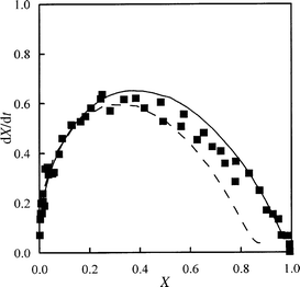Fig. 7 Dimensionless conversion rate vs. conversion for marine char. Symbols, experimental data; solid line, two-dimensional simulation by CA; dashed line, traditional numerical simulation. The CA results are the mean values of 50 different runs.

Fig. 8 reports the comparison between two simulation runs performed on marine char. In the first run, shown as a dashed line, micropores were filled (at 50%) with reacting gas ‘‘r ’’. In the second run, shown as a solid line, micropores were filled (at 50%) with non-reacting gas ‘‘p’’. As can be seen, the hypothesis that micropores are not available for reaction is confirmed from the simulation results. Indeed, only the second simulation run is capable of predicting the experimental trend.

Fig. 8 Test of hypothesis that micropores are unavailable for the reaction. Marine char 2D simulation. Dashed line, simulation performed by filling the micropores (at 50%) with ‘‘r’’ reacting gas particles; solid line, simulation performed by filling the micropores (at 50%) with ‘‘p’’ non-reacting gas particles.

In Fig. 9, results for 2D simulations are reported for the Spherocarb case. Also for this char CA simulation describes the experimental results very well and quantitatively. In Fig. 10 the graphite conversion rate is plotted against conversion. A good comparison between 2D simulation and experiment can also be noted.

Fig. 9 Dimensionless conversion rate vs. conversion for Spherocarb. Symbols, experimental data; solid line, two-dimensional simulation by CA; dashed line, traditional numerical simulation. The CA results are the mean values of 50 different runs.

Fig. 10 Dimensionless conversion rate vs. conversion for graphite. Symbols, experimental data; solid line, two-dimensional simulation by CA; dashed line: traditional numerical simulation. The CA results are the mean values of 50 different runs.

In Fig. 11, the 3D simulations for the three chars are reported. The results do not exhibit important differences from the 2D simulations. Consequently, also in this case the agreement with experiments is very good. In Fig. 12, the ratio of overall active surface A to initial active surface A₀ for 3D simulation is reported against the number of execution steps n (i.e., time). On the plots, the standard deviation and the mean value of each set of 50 runs are reported. As can be seen, the standard deviation increases toward the end of the runs where only a small number of pixels are left to react. The diagrams indicate that 50 runs in each case are sufficient for statistical significance of the simulated process.

Fig. 11 Simulation results for the 3D case. From top to bottom: marine char, graphite and Spherocarb. Symbols, experimental data; solid line, three-dimensional simulation by CA.

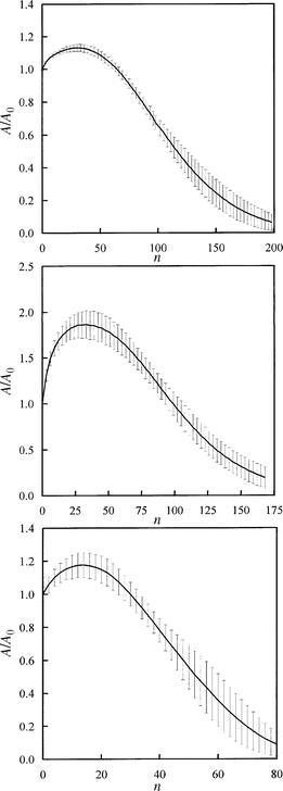Fig. 12 Ratio between active surface area and initial active surface area vs. execution steps for the 3D simulations. Standard deviations are plotted as error bars. From top to bottom: marine char, graphite and Spherocarb.

Overall, the CA approach appears to be a promising tool for the simulation and analysis of heterogeneous reaction processes. The ambitious objective of obtaining CA quantitative simulations of the heterogeneous reactive process has indeed been reached, as the results clearly indicate. Quantitative results can be predicted for chars of significantly different porosity. The essence of the process (random gas movement, gas–solid interaction, surface progressive erosion) can be well described at a fine grain level (though only at a mesoscopic scale because of hardware limitations) by the logical parallel operation of each elementary automaton. As shown in this work, for the description of the reacting system, the CA model is completely different from the continuous traditional model and lends itself to fast massive parallel computing. The application of CA appears to be useful in cases where the traditional method, based on the numerical integration of stiff partial differential equations sets, cannot be implemented at a significant degree of detail, owing to extremely time-consuming computations.

Acknowledgements

This work was performed in the frame of activities of the CNR Institute of Research on Membrane and Chemical Reactor Modeling and was partially funded by the CNR Finalized Project ‘‘Chimica Fine II’’ and by the Ministry of University and of Scientific Research of Italy.

References

1. N. R. Amudson and S. W. Sotirchos, AIChE J., 1984, 30, 4.
2. S. K. Bathia and D. D. Perlmutter, AIChe J., 1980, 26, 379..
3. A. Lindenmayer, presented at the IVth International Congress for Logic, Methodology and Philosophy of Science, Bucharest, 1971..
4. J. Von Neumann, Theory of Self Reproducing Automata, University of Illinois Press, Urbana, 1966..
5. U. Frisch, B. Hasslacher and Y. Pomean, Phys. Rev. Lett., 1986, 56, 1505.
6. T. Toffoli and N. Margolus, Cellular Automata Machines, MIT Press, Cambridge, MA, 1987..
7. R. Said and R. Borghi, in Proceedings of the Twenty-Second International Symposium on Combustion, The Combustion Institute, Pittsburgh, PA, 1988, p. 569..
8. S. Chen, S. P. Dawson, G. D. Doolen, D. R. Janecky and A. Lawniczak, Comput. Chem. Eng., 1995, 19, 617.
9. M. J. Biggs and S. J. Humby, Chem. Eng. Res. Des., 1998, 76, 162.
10. J. M. Smith, Chemical Engineering Kinetics, McGraw-Hill, Singapore, 1981..
11. S. P. Nandi and P. L. Walker Jr., Fuel, 1970, 49, 309.
12. G. R. Gavalas, AIChE J., 1980, 26, 577.
13. M. D' Amore, F. P. Di Maio, P. G. Lignola and S. Masi, Combust. Sci. Technol., 1993, 89, 71.
14. E. B. Dynkin and A. A. Yushkevich, Markov Processes, Plenum Press, New York, 1969..

---