Discrimination of chemically similar organic vapours and vapour mixtures using the Kohonen network

Abstract

A Kohonen network was employed to discriminate between a series of chemically similar alcohols and mixtures of organic solvents. The input data for the Kohonen analysis was generated using an optimized eight-sensor array designed to sample the headspace of the solvents. Different sizes of output grid were investigated to devise a network that gave optimum discrimination and maintained relationships within the data set. When the output grid was large compared to the number of classes in the sample set, discrimination was shown to be enhanced compared to a small output grid. An advantage of the small output grid is that it was shown to maintain information within the original data set. The Kohonen network generated easily distinguishable output patterns, which could be used as an alternative to pattern recognition or in conjunction with output grid maps.

---

Introduction

The raw sensor responses obtained from an array of non-specific gas sensors are generally insufficient to discriminate between a series of samples unless they are very diverse. Because of this limited discrimination, pattern recognition methods are normally used to enhance differences between raw sensor outputs. Linear statistical methods which have been used in conjunction with sensor arrays include linear multivariate techniques such as cluster analysis (CA), principal component analysis (PCA) and discriminant function analysis (DFA).^1,2 Alternatively, non-linear pattern recognition methods, such as artificial neural networks (ANNs), e.g., back-propagation networks,^3–18 and self-organized maps (SOMs), e.g., Kohonen networks,^19–22 have been used. Often the success of the approach is heavily dependent on the specific application; for example, some array sensors generate linear responses while others are obviously non-linear. Deciding on the correct data processing method is not always straightforward because the measured sensor responses may result from more than one process. For instance, when linear data processing methods are used for data obtained from nominally linear sensor responses, any non-linear sensor drift cannot be accounted for.

In general, PCA and DFA are the preferred linear data reduction methods in multivariate analysis. Both techniques are suitable for relatively small data sets and, in both instances, two-dimensional feature plots can be generated which display clusters of similar samples. Alternatively, the similarity (or differences) between the samples can also be expressed as the distance in feature space. Unfortunately, the data reduction process employed by both techniques to enhance the differences between test sample data may result in the loss of useful information and the inclusion of artefacts such as sensor drift and sensitivity changes. In extreme cases, these failings may cause misclassification of an unknown sample. Non-linear pattern recognition methods such as back-propagation networks are useful for compensating for sensor drift. However, such networks require large data sets, which may not be practical.

In an attempt to circumvent the problems discussed above, Kohonen self-organizing maps were employed in this work as a non-linear data processing method. The technique was also chosen on the basis of its suitability for small data sets, the simple output data generated and, more importantly, to avoid data reduction.

The sensor array used in this study consisted of eight sorbent-coated quartz crystal microbalance sensors designed to cover all solvation interactions. The sensor specifications and the design criteria for the array are described in an earlier publication. In the same paper, we have demonstrated that the sensor array can be used to classify a diverse range of volatile organic compounds (VOCs) using PCA and DFA as the data processing methods. Both data reduction techniques maximized differences between samples and generated two-dimensional feature plots. This ‘general purpose’ array configuration contains a wide spread of sensor functions and gave good resolution of test samples with diverse chemical functionalities, but was less successful in the discrimination of test sets containing chemically and physically similar compounds. In order to discriminate between chemically similar samples, it was necessary to ‘tune’ the array by disabling certain sensor inputs so that the variance was maximized for the remaining sensors.

In a more recent paper,²⁴ we have investigated the feature extraction capabilities of a Kohonen network in conjunction with a quartz crystal gas sensor array. The network discriminated between 12 organic vapours containing diverse chemical functionalities. The output grid map showed that samples were linked in feature space with respect to their relative interaction strengths, which suggested that relationships within the input data were maintained.

In this paper, a range of test samples was chosen to demonstrate the ability of Kohonen self-organizing maps to discriminate chemically between similar analytes, maintain relationships in data and handle relatively small data sets.

Experimental

Reagents and materials

Eight piezoelectric quartz crystals were coated with different sorbent layers: poly(isobutylene) (PIB), poly(epichlorohydrin) (PECH), poly(propylene glycol) (PPG) (Aldrich, Dorset, UK); cyano-substituted polysiloxane OV225, phenylallylphenyl-hexafluoropropane (Allyl-Bis), poly(2,3,4-hexafluoropentane-1,5-diol-co-epichlorohydrin) (PPE) and poly(ethylene maleate) (PEM) (synthesized).

Three sample test sets comprised: (A) methanol, ethanol, propan-1-ol, propan-2-ol, n-butanol; (B) 5% toluene in xylene, 10% toluene in xylene, 50% toluene in xylene; 90% toluene in xylene, 95% toluene in xylene; (C) 1% dichloromethane in toluene, toluene, 1% toluene in dichloromethane and dichloromethane. All solvents were Analar grade from Merck (Poole, Dorset, UK). The sample containers were 1.5 ml polypropylene vials (Sarstedt, Leicester, UK).

Instrumentation

The sensor response data were collected on a QTS-1 sensor array system (Quartz Technology Limited, Northwood, UK) using an interchangeable array of eight sensors (described above). The system generates comma separated variable (CSV) data files containing the response of the frequency elements (F(t))_s1–(F(t))_{s 8} [where (F(t))_s1 is the frequency response of sensor 1 and so forth] of each individual sensor over the time course (t) of an experiment. These data files were exported to Excel (Microsoft Corporation, Redmond, WA, USA) and Neuroshell 2 (Ward Systems Group, Inc., Frederick, MD, USA) for data analysis.

Kohonen network configurations

The Kohonen network is designed to accept preprocessed data (scaled responses) with predefined target values. In this work, scaled responses [(ςf/Σ(ςf_s1– ςf_s8) where ςf = F(t) − F(0)] were used as input where t = 30 s. The target values onto which the input data were mapped were set between the mean minus two times the standard deviation (x̄ − 2ς) and the mean plus two times the standard deviation (x̄ + 2ς). Normally, the number of nodes in the Kohonen output layer (grid size) is chosen on the basis of the number of groups to be distinguished. In general, a few hundred epochs (training cycles) are sufficient to train the network compared to the thousands of cycles required by some ANNs, such as back-propagation.

The Kohonen networks employed for the classification of all organic vapour sample sets consisted of eight inputs and a varying number of outputs. The training set consisted of 15 patterns for sample sets A and B and eight patterns for sample set C. The test set consisted of 10 patterns for sample sets A and B and eight patterns for sample set C. The output layer consisted of four nodes (2 × 2 grid), nine nodes (3 × 3 grid), 16 nodes (4 × 4 grid) and 25 nodes (5 × 5 grid). The neighbourhood size was defined by the number of nodes in the output layer, the learning rate was set to 0.5, the initial weight settings were −0.5 to 0.5, and the network was trained for 100 epochs. Training patterns were selected randomly to maximize oscillation in the training process and to generate a robust model.

Results and discussion

The first step of the process involves generating training node weight patterns from sensor responses. The sample test sets are compared to the training node weight patterns and matched patterns are deemed winners of that particular node. Essentially, the output pattern generated by the Kohonen network is the difference between the input pattern and the winning node weight pattern. For a successful discrimination of different sample types, each type should occupy a different node.

Sample set A contained five simple aliphatic alcohols (methanol, ethanol, propan-1-ol, propan-2-ol and n-butanol) with increasing numbers of carbon atoms. The chemical and physical properties of this class of compounds are well documented with certain parameters, for example, boiling points, reflecting their molecular weight and intermolecular interactions. The composition of the sample test set was designed to assess the power of the Kohonen network to discriminate between analytes which are chemically and structurally similar, and to show that relationships in the input data are maintained.

Sample set B contained a series of toluene–xylene mixtures. The components were chosen because they are chemically and physically very similar compounds, they form ideal solution mixtures and are inherently difficult to discriminate. The choice of samples also facilitated an investigation of the vapour pressure–mole fraction relation for ideal mixtures.

Sample set C contained four samples: 1% dichloromethane in toluene, toluene, 1% toluene in dichloromethane and dichloromethane. This sample set was designed as an example of a test of the capability of the Kohonen network to discriminate a pure sample from a slightly contaminated sample.

The effects of output grid size on discrimination ability were demonstrated using sample set A. The results (Figs. 1 and 2) suggest that optimum discrimination requires an output grid with a significantly greater number of nodes than the number of samples to be discriminated. However, there is a limit to the maximum grid size that can be used, because employing an excessively large output grid tends to result in multiple winning nodes and the final output can be confusing. In this example, three grid sizes (3 × 3, 4 × 4 and 5 × 5) achieved adequate discrimination of the five alcohols. For the two smaller grids, a specific node number was assigned to a particular alcohol and there were no multiple winning nodes or shared nodes among samples [Figs. 1(a) and 1(b)]. The larger 5 × 5 grid also discriminated between the samples successfully (no shared node), but resulted in some multiple winning nodes. A comparison of the three outputs shows that the larger the output grid used, the further apart the winning nodes are from each other, thereby reducing the risk of having shared winning nodes between different samples. Furthermore, the output pattern of propan-1-ol showed that there was competition between node number 8 and 17, with the latter node being the winner. In fact, the output patterns of methanol, ethanol, propan-1-ol and propan-2-ol revealed multiple troughs which may suggest competition among nodes leading to dispersion of ‘winners’. The winners of the 4 × 4 output grid [Fig. 1(b)] were well separated and there was no dispersion of winning nodes, which suggested that optimum discrimination of the samples was achieved. It was concluded that the selection of a suitable output grid size was crucial for reliable discrimination. For this array, a useful ‘rule of thumb’ was that the grid size should be 3n where n is the number of samples in the class.

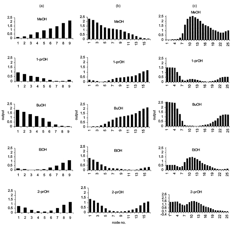Fig. 1 Output patterns in Kohonen 3 × 3 (a), 4 × 4 (b) and 5 × 5 (c) grids obtained for sample set A.

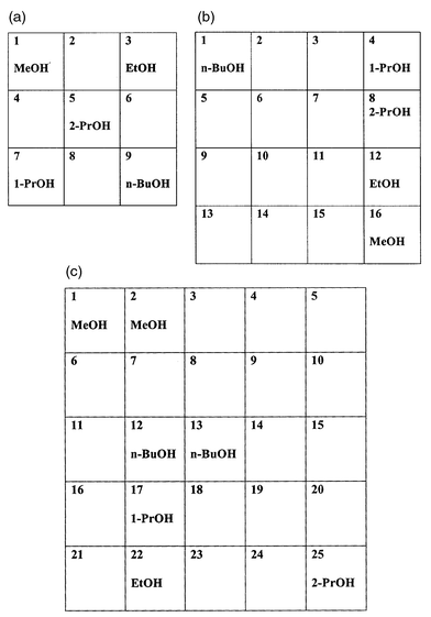Fig. 2 Kohonen 3 × 3 (a), 4 × 4 (b) and 5 × 5 (c) output grids showing the winning node number for each sample from a test set of five different alcohols.

The output from the Kohonen network can also be represented as feature maps. The feature maps maintain natural relationships within input data through multidimensional links within the feature spaces of the output map. The outputs (winning node numbers) from the five alcohols for each sample are presented as a 3 × 3, 4 × 4 and 5 × 5 grid feature maps in Figs. 2(a)–2(c). The 3 × 3 grid feature map [Fig. 2(a)] shows a uniform dispersion of winners with the propan-2-ol samples havingmultiple links with all other samples. This linkage pattern suggests that this particular branched alcohol is the most distinct sample within the test set. The limited number of nodes available with this grid size obscures any other relationships within the test set. The 4 × 4 output grid map [Fig. 2(b)] revealed linear two-dimensional links among four alcohols with the exception of n-butanol. The observed deviation of n-butanol from the other samples may be due to the limited feature space available in the map. Since the four alcohols occupied all available spaces within a particular column of the 4 × 4 grid map, n-butanol was forced into the second best feature space. The 5 × 5 grid map revealed a loss of meaningful links between some samples [Fig. 2(c)]. This is probably a result of the network breaking down because of an excessively large output grid size; the results are similar to those shown in Fig. 1(c).

A comparison of the number of carbon atoms in the test compounds against the winning node number [Figs. 3(a) and 3(b)] is similar to the trend observed when boiling point is compared with the number of carbon atoms for the same set of alcohols [Fig. 3(d)]. Since the boiling point is a reflection of the molecular properties, such as the strength of dispersion interactions, it is probable that the energy of interaction between sorbents and test vapour molecules was predominant in determining the sensor responses. This suggests that the solvation model employed for developing our sensor array is realistic.

Fig. 3 Kohonen output [3 × 3 (a), 4 × 4 (b) and 5 × 5 (c) grids] winning node–concentration plots for a series of five alcohols. [For (c), ■ and ◆ are multiple winning nodes.] (d) Boiling point versus number of carbons in methanol, ethanol, propan-1-ol, propan-2-ol and n-butanol.

The Kohonen network was applied to data obtained on exposure of the sensor array to a series of five organic mixtures (5%, 10%, 50%, 90% and 95% v/v toluene in xylene). In this analysis, 3 × 3 and 4 × 4 output grids were used to avoid multiple winning nodes. The output patterns generated by both Kohonen networks [Figs. 4(a) and 4(b)] show that discrimination of samples was better with the 4 × 4 grid. The winning nodes in the 4 × 4 grid map were better separated and hence the patterns were more readily distinguished.

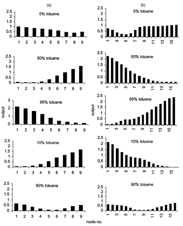Fig. 4 Output patterns in Kohonen 3 × 3 (a) and 4 × 4 (b) grids obtained for sample set B.

The same feature map presentation [Fig. 5(b)] and a plot of concentration versus winning node number [Fig. 5(a)] were used to demonstrate the ability of the Kohonen network to retain relationships in the data set. The feature map clearly distinguished all samples and the plot [Fig. 5(a)] was linear between 10% toluene and 90% toluene, but deviations were observed for 5%–10% toluene in xylene and 90%–95% toluene in xylene. The latter observations may be due to artefacts of the sensor system, or some undesirable changes within the sensors, mainly due to visco-elastic effects. The sensitivity of the sensors coated with PIB and the two silicone oils (OV25 and OV225) is more likely to be affected by visco-elastic changes when they interact with volatile aromatic hydrocarbons. When the concentration of component is ⩾10%, no further visco-elastic changes are expected to occur, and the output data reflect the concentration of the samples. Unfortunately, the occurrence of artefacts is an unavoidable limitation for all chemical sensing devices which are based on a signal generated by a secondary sensing mechanism, instead of directly generated from the analyte itself as, for example, in the case of infrared spectroscopy.

Fig. 5 (a) Kohonen output [4 × 4 (A) and 3 × 3 (B) grids] winning node–concentration plot for a series of toluene–xylene mixtures. (b) Kohenen output (4 × 4 grid) showing winning nodes for a series of toluene–xylene mixtures.

Sample set C was chosen to provide two pure samples with different functionalities together with a contaminated sample (1% dichloromethane in toluene, toluene, 1% toluene in dichloromethane and dichloromethane). A 2 × 2 and a 3 × 3 output grid were used for this sample set of four analytes. The larger grid size was found to be useful for maximizing the discrimination of the samples. The 2 × 2 output grid [Fig. 6(a)] failed to discriminate between toluene and the ‘doped’ toluene (both samples won node 1) and their output patterns were also indistinguishable. The 3 × 3 output grid [Fig. 6(b)] improved the discrimination between the samples by assigning each sample into a different node number (winning nodes: 1, 4, 8 and 9, respectively) and the differences between the output patterns were also improved. The individual output patterns in Fig. 6(b) clearly showed that each of the two pure samples adopted different patterns, while the similarity between the pure and the doped samples of the individual compounds were maintained. The grid map in Fig. 6(c) suggested that there was a link between the two doped samples which contained common components, but the two pure samples were obviously different from each other.

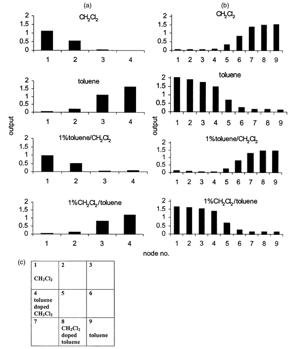Fig. 6 Output patterns in Kohonen 2 × 2 (a) and 3 × 3 (b) grids obtained for sample set C. (c) Kohonen 3 × 3 output grid map obtained for sample set C.

Conclusions

The Kohonen network was shown to be an effective feature extraction method, which was capable of retaining relationships in the input data. The Kohonen output map was used to discriminate between chemically similar compounds (alcohols of different chain lengths), organic vapour mixtures (mixtures of toluene and xylene) and contaminated organic solvents (contaminated toluene and dichloromethane). It was found that the configuration of the network was important for obtaining the optimum resolution for a given sample set with similar properties. For example, an output grid size of around three times the number of samples to be discriminated was required to achieve good resolution.

The Kohonen network was shown to cope with small data sets and meaningful results were obtained. It was found that, when appropriate configurations were chosen for a particular test set, both the output grid and the output patterns were useful for sample discrimination. The ability of the Kohonen network to retain input data was demonstrated in all three examples. The relationship between the winning node number and the number of carbons in the five alcohols is a reflection of the relative solvation energy for the alcohols (Fig. 3).

The output from the toluene–xylene mixtures resulted in a plot which contained a linear region expected for ideal mixtures [Figs. 5(a) and 5(b)]. The pure and doped toluene and dichloromethane samples in sample set C were resolved and the grid map indicated some similarities between the two cross-contaminated samples.

References

1. J. R. Stetter, P. C. Jurs and S. L. Rose, Anal. Chem., 1986, 58, 860.
2. S. L. Rose-Pehrsson, J. W. Grate, D. S. Ballantine, Jr. and P. C. Jurs, Anal. Chem., 1988, 60, 2801.
3. H. Nanto, T. Kawai, H. Sokooshi and T. Usuda, Sens. Actuators B, 1993, 13–14, 718.
4. T. Nakomoto, K. Fukunishi and T. Moriizumi, Sens. Actuators B, 1990, 1, 473.
5. T. Nakamoto, A. Fukuda and T. Moriizumi, Sens. Actuators B, 1993, 10, 85.
6. B. W. Saunders, D. V. Thiel and A. Mackay-Sim, Analyst, 1995, 120, 1013.
7. J. Auge, P. Hauptmann, J. Hartmann, S. Rosler and R. Lucklum, Sens. Actuators B, 1995, 24, 43.
8. H. Nanto, S. Tsubakino and M. Endo, Sens. Actuators B, 1995, 24–25, 794.
9. A. Hierlemann, U. Weimar, G. Kraus, M. Schweizer-Berberich and W. Gopel, Sens. Actuators B, 1995, 26–27, 126.
10. J. W. Gardner, H. V. Shurmer and T. T. Tan, Sens. Actuators B, 1992, 6, 71.
11. C. Di Natale, F. A. M. Davide and A. D’Amico, Sens. Actuators B, 1994, 18–19, 244.
12. H. Endres, W. Gottler, H. D. Jander, S. Drost, G. Sberveglieri, G. Faglia and C. Perego, Sens. Actuators B, 1995, 24–25, 785.
13. T. Nakamoto, H. Takagi, S. Utsumi and T. Moriizumi, Sens. Actuators B, 1992, 8, 181.
14. E. L. Hines and J. W. Gardner, Sens. Actuators B, 1994, 18–19, 661.
15. S. W. Moore, J. W. Gardner, E. L. Hines, W. Gopel and U. Weimar, Sens. Actuators B, 1993, 15–16, 344.
16. D. Rebiere, C. Bordieu and J. Pistre, Sens. Actuators B, 1995, 24–25, 777.
17. B. Hivert, M. Hoummady, J. M. Henrioud and D. Hauden, Sens. Actuators B, 1994, 18–19, 645.
18. V. Sommer, P. Tobias and D. Kohl, Sens. Actuators B, 1993, 12, 147.
19. T. Kohonen, Self-Organization and Associative Memory, Springer Verlag, Berlin, 3rd edn., 1989..
20. D. R. Bull, G. J. Harris and A. B. Ben Rashed, Sens. Actuators B, 1993, 15–16, 151.
21. C. Di Natale, F. A. M. Davide, G. Faglia and P. Nelli, Sens. Actuators B, 1995, 23, 187.
22. J. Zupan, M. Novic, X. Li and J. Gasteiger, Anal. Chim. Acta, 1994, 292, 219.
23. K. T. Lau, J. Micklefield and J. M. Slater, Sens. Actuators B, 1998, 50, 69.
24. P. McAlernon, J. M. Slater and K. T. Lau, Analyst, 1999, 124, 851.

---

Footnote

† Presented at SAC 99, Dublin, Ireland, July 25–30, 1999.

---