The interplay between activity and filament flexibility determines the emergent properties of active nematics

Abstract

Active nematics are microscopically driven liquid crystals that exhibit dynamical steady states characterized by the creation and annihilation of topological defects. Motivated by differences between previous simulations of active nematics based on rigid rods and experimental realizations based on semiflexible biopolymer filaments, we describe a large-scale simulation study of a particle-based computational model that explicitly incorporates filament semiflexibility. We find that energy injected into the system at the particle scale preferentially excites bend deformations, reducing the apparent filament bend modulus. The emergent characteristics of the active nematic depend on activity and flexibility only through this activity-renormalized bend ‘modulus’, demonstrating that apparent values of material parameters, such as the Frank ‘constants’, depend on activity. Thus, phenomenological parameters within continuum hydrodynamic descriptions of active nematics must account for this dependence. Further, we present a systematic way to estimate these parameters from observations of deformation fields and defect shapes in experimental or simulation data.

---

I. Introduction

Active nematics are a class of non-equilibrium liquid crystalline materials in which the constituent particles transduce energy into stress and motion, driving orientationally inhomogeneous dynamical steady states characterized by generation, annihilation, and streaming of topological defects.^1–7 Being intrinsically far-from-equilibrium, active nematics enable developing materials with capabilities that would be thermodynamically forbidden in an equilibrium system. However, such applications require understanding how an active nematic's macroscale material properties depend on the microscale features of its constituent nematogens.

The challenge in this task can be illustrated by considering the shape of a defect. Defects have been the subject of intense research in equilibrium nematics, since they must be eliminated for display technologies, and controlled for applications such as directed assembly and biosensing.^8–10 Theory and experiments^10–12 have shown that defect morphologies depend on the relative values of the bend and splay elastic moduli, k₃₃ and k₁₁ (Fig. 1a), defined in the Frank free energy density for a 2D nematic as f_F = k₁₁(∇·n̂)² + k₃₃(n̂ × (∇ × n̂))² with n̂ the director field.^13,14 Different experimental realizations of active nematics also exhibit variations in defect morphologies (e.g.Fig. 1c and d). However, relating these defect morphologies to material constants is much less straightforward than in equilibrium systems. Since moduli are an equilibrium concept, they cannot be rigorously defined in a non-equilibrium system such as an active nematic. If it is possible to define ‘effective moduli’ in active systems, there is currently no systematic way to measure them, and it is unclear whether and how they may depend on activity.

Fig. 1 (a and b) The equilibrium director field configuration near a +½ defect for (a) bend modulus larger than splay modulus k₃₃/k₁₁ = 3.4, leading to pointed defects and (b) splay modulus larger than bend k₃₃/k₁₁ = 0.3 leading to rounded defects. In each case the director field was calculated by numerically minimizing the Frank free energy around a separated ±½ defect pair. (c and d) Typical defect morphologies observed in (c) a vibrated granular nematic⁵ and (d) a microtubule-based active nematic.^1,40

Computational and theoretical modeling could overcome these limitations. Symmetry-based hydrodynamic theories^15–17 have led to numerous insights about active nematics, including describing defect dynamics (e.g.ref. 18–23), induced flows in the suspending fluid (e.g.ref. 24–26), and how confinement in planar^27–30 and curved geometries^31–34 controls defect proliferation and dynamics. However, hydrodynamic theories cannot predict how material constants or emergent behaviors depend on the microscale properties of individual nematogens. Further, while simulations of active nematics composed of rigid rods^2,35–37 have elucidated emergent morphologies, these models do not account for internal degrees of freedom available to flexible nematogens.^1,38,39

In this work, we perform large-scale simulations on a model active nematic composed of semiflexible filaments, and determine how its emergent morphology depends on filament stiffness and activity. Fig. 2 shows representative simulation outcomes. We find that the intrinsic bending modulus of nematogens κ undergoes an apparent softening in an active nematic, according κ_eff ∼ κ/(f^a)², where f^a is a measure of its activity. Furthermore, the characteristics of the active nematic texture – the defect density, magnitudes and characteristic scales of bend and splay deformations, the shape of motile defects, and number fluctuations – depend on activity and rigidity only through the apparent nematogen rigidity κ_eff. Moreover, we show that one can define effective bend and splay moduli analogous to their equilibrium counterparts, but that the apparent bend modulus is proportional to κ_eff. This observation demonstrates that activity preferentially dissipates into particular modes within an active material, depending on the internal degrees of freedom of its constituent units. Further, these results suggest revisiting assumptions underlying existing hydrodynamic theories of active matter, since a microscopic model for an active fluid results in macroscopic properties that depend on activity in nontrivial ways, which cannot be simply described by an active stress. Finally, we present a method of parameterizing defect shapes, which enables estimating the relative magnitudes of apparent bend and splay constants from experimental observations of defects, and thus allows direct experimental testing of our prediction.

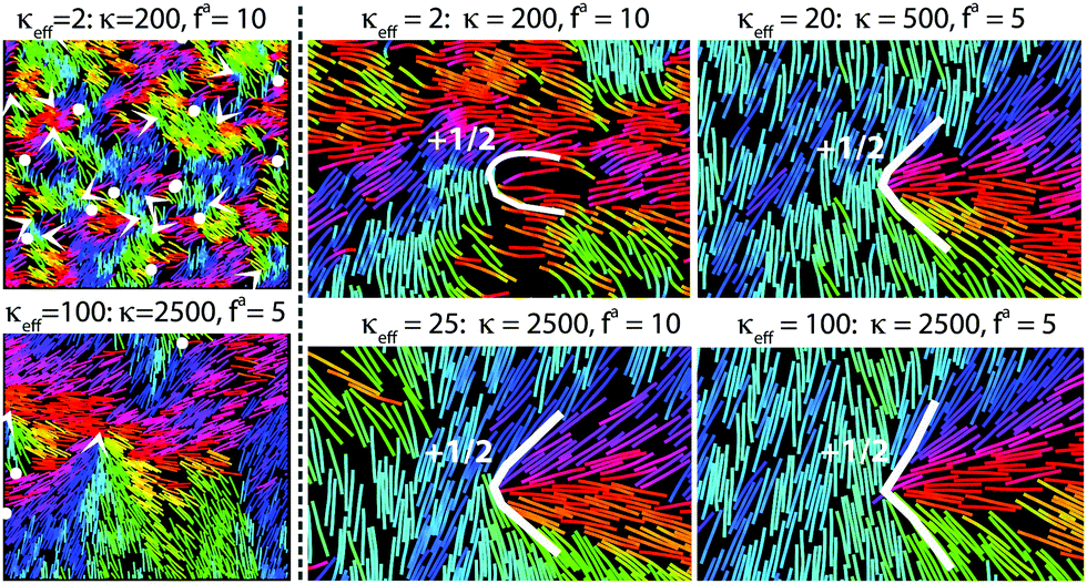Fig. 2 A visual summary of how active nematic emergent properties depend on the activity parameter f^a and the filament modulus κ. The left panel in each row shows 1/16th of the simulation box for indicated parameter values, with white arrows indicating positions and orientations of +½ defects and white dots indicating positions of -½ defects. Filament beads are colored according to the orientations of the local tangent vector. The right 4 panels are each zoomed in on a +½ defect, with indicated parameter values. The white lines are drawn by eye to highlight defect shapes. Animations of corresponding simulation trajectories are in the ESI.†⁴¹ The box size is (840 × 840σ²) for all simulations in this work. Other parameters are τ₁ = 0.2τ and k_b = 300k_BT_ref/σ².

II. Methods

We seek a minimal computational model that captures the key material properties and symmetries of active nematics, namely extensile activity, nematic inter-particle alignment and semiflexibility. We model active filaments as semiflexible bead-spring polymers, each containing M beads of diameter σ, with flexibility controlled by a harmonic angle potential between successive bonds that sets the filament bending modulus κ. Activity is implemented as a force of magnitude f^a acting on each filament bead along the local tangent to the filament. To make activity nematic, the active force on every bead within a given filament reverses direction after a time interval chosen from a Poisson distribution with mean τ₁. The Langevin equations governing the system dynamics were integrated using a modified version of LAMMPS.⁴² The model combines features of recent models for polar self-propelled polymers⁴³ and the reversing rods approach to rigid active nematic rods.³⁶

Equations of motion and interaction potentials

We simulate the dynamics according to the following Langevin equation for each filament α and bead i (with filaments indexed by Greek letters, α = 1,…,N, and beads within a filament indexed in Roman, i = 1,…,M):

mr̈_α,i = f^a_α,i − γṙ_α,i − ∇_rα,iU + R_α,i(t). (1)

with m as the bead mass, r_α,i as the bead position, f^a as the active force, U as the interaction potential which gives rise to the conservative forces, γ as the friction coefficient providing the damping and R_α,i(t) as a delta-correlated thermal noise with zero mean and variance 〈R_α,i(t)·R_β,j(t′)〉 = 4γk_BTδ_α,βδ_ijδ(t − t′).

The interaction potential includes three contributions which respectively account for non-bonded interactions between all bead pairs, stretching of each bond, and the angle potential between each pair of neighboring bonds:

with θ_α,i,j,k the angle made by the bead triplet {i, j, k} on filament α. The non-bonded interactions account for steric repulsion and are modeled with the Weeks–Chandler–Anderson potential⁴⁴

U_nb(r) = 4ε((σ/r)¹² − (σ/r)⁶ + 1/4)Θ(2^1/6σ − r) (3)

with ε controlling the strength of steric repulsion and Θ(x) the Heaviside function specifying the cutoff. Bond stretching is controlled by a FENE potential⁴⁵

U_s(r) = −1/2k_bR₀² ln(1 − (r/R₀)²) (4)

with bond strength k_b and maximum bond length R₀. The angle potential is given by

U_angle(θ) = κ(θ − π)² (5)

where κ is the filament bending modulus.

Finally, activity is modeled as a propulsive force on every bead directed along the filament tangent toward its head. To render the activity nematic, the head and tail of each filament are switched at stochastic intervals so that the force direction on each bead rotates by 180 degrees. In particular, the active force has the form, f^a_α,i(t) = η_α(t)f^at_α,i, where f^a parameterizes the activity strength, and η_α(t) is a stochastic variable associated with filament α that changes its values between 1 and −1 on Poisson distributed intervals with mean τ₁, so that τ₁ controls the reversal frequency.

Simulations and parameter values

Since we are motivated by systems sufficiently large that boundary effects are negligible (e.g.ref. 2), we performed simulations in a A = 840 × 840σ² periodic simulation box, with N = 19 404 filaments, each with M = 20 beads, so that the packing fraction ϕ = MNσ²/A ≈ 0.55. Fixing all other model parameters, we varied the filament stiffness, κ ∈ [10², 10⁴]k_BT_ref and the magnitude of the active force, f^a ∈ [5, 30]k_BT_ref/σ, where the units are set by the thermal energy at a reference state k_BT_ref, and the filament diameter σ. Time is measured in units of . We set mass of the each bead to m = 1, the damping coefficient to γ = 2, and the temperature to T = 3.0k_BT_ref. With these parameters inertia is non-negligible. In the future, we plan to systematically investigate the effect of damping. We set the repulsion parameter ε = k_BT_ref (the results are insensitive to the value of ε provided it is sufficiently high to avoid filament overlap), and used a time step of δt = 10⁻³τ.

In the FENE bond potential, R₀ is set to 1.5σ and k_b = 300k_BT_ref/σ² for the simulations reported in the main text (except in Fig. 3). These parameters lead to a mean bond length of b ≈ 0.84σ, which ensures that filaments are non-penetrable for the parameter space explored in this work. We have fixed the filament length at M = 20 beads, so L = (M − 1)b is the mean filament length. Varying M does not change the scaling of observables, although it shifts properties such as the defect density since the total active force per filament goes as f^aM. Also, the maximum persistence length above which scaling laws fail is proportional to M (see Results). In the semiflexible limit, the stiffness κ in the discrete model is related to the continuum bending modulus as , and thus the persistence length is given by l_p = 2bκ/k_BT.

Fig. 3 Effective persistence length l_p estimated from the spectrum of filament tangent fluctuations in bulk active nematics (large open symbols), and isolated chains (small solid symbols). The dashed line shows the expected scaling for an isolated equilibrium polymer (f^a = 0), l_p = 2bκ_eff/k_BT, and the legend shows the value of f^a for all systems, and κ for the bulk simulations. Other parameters are τ₁ = τ and k_b = 30k_BT_ref/σ².

We performed two sets of simulations. Initially, we set the FENE bond strength k_b = 30k_BT_ref/σ² and τ₁ = τ. However, for these parameters we discovered that interpenetration of filaments becomes possible at large propulsion velocities, thus limiting the simulations to f^a ≤ 10. To enable investigating higher activity values, we therefore performed a second set of simulations (those reported in Fig. 4–7 of the main text) with higher FENE bond strength, k_b = 300k_BT_ref/σ² and shorter reversal timescale τ₁ = 0.2, with κ ∈ [100, 10 000]k_BT_ref. This enables simulating activity values up to f^a ≤ 30.

Fig. 4 Analysis of splay and bend deformations at steady state: (A) the ratio of splay and bend deformations, as a function of the effective bending rigidity, κ_eff = κ/(1 + (f^a)²). (B) The wavenumbers corresponding to peaks k_peak in bend ( symbols) and splay ( symbols) power spectra, and the inverse defect spacing, ( symbols) as functions of κ_eff. The predominant scale of splay deformations transitions from the individual filament scale (k_filament, dashed line) at low κ_eff to the defect spacing scale at high κ_eff. Bend spectra exhibit two peaks, corresponding to filament and defect-spacing scales, for high κ_eff. (C) The maximum magnitude of the power spectra, showing that splay is insensitive to κ_eff while bend deformations decrease in magnitude until the effective rigidity exceeds the filament length. Other parameters are τ₁ = 0.2τ and k_b = 300k_BT_ref/σ².

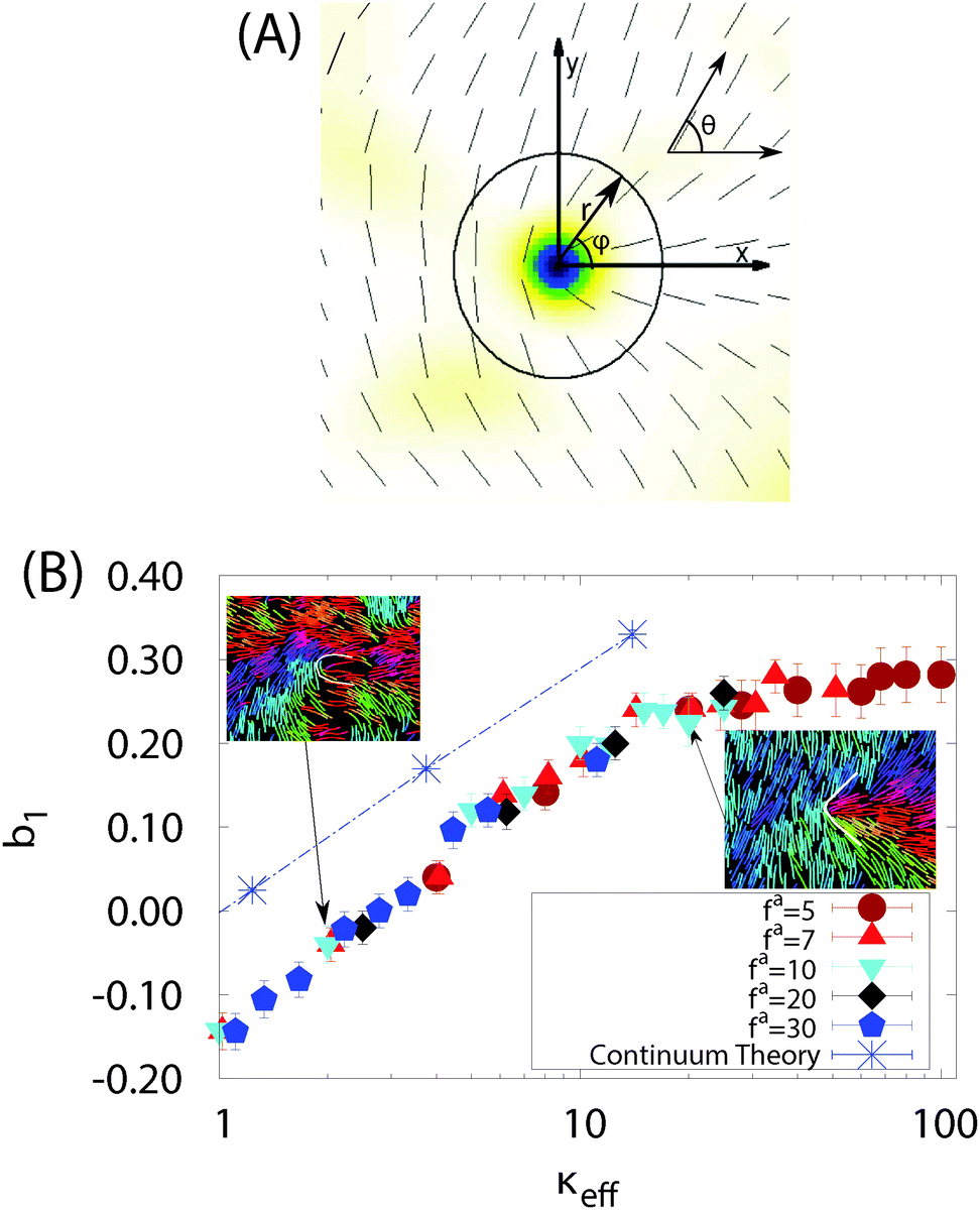Fig. 5 Defect shape depends on the effective bending rigidity. (A) Schematic showing the defect-centered coordinate system defined in the text, with azimuthal angle ϕ and director angle θ(r, ϕ). Note that the x-axis is chosen along the orientation vector of the +1/2 defect given by the angle θ₀′ defined in the ESI.†⁴¹ (B) Mode of defect shape parameter b₁ for +½ defects as a function of κ_eff for f^a ∈ [7, 30] and κ ∈ [100, 10 000], with b₁(r) values evaluated at a radial distance r = 12.6σ from the defect core. The dashed line and blue asterisk symbols show values of b₁ calculated for isolated defects from equilibrium continuum elastic theory, with the ratio of bend and splay moduli k₃₃/k₁₁ for each κ_eff set according to the measured ratio R of bend and splay deformations in Fig. 4. Images of defects at two indicated parameter sets are shown. Other parameters are τ₁ = 0.2τ and k_b = 300k_BT_ref/σ².

Fig. 6 The average number of defects n_defect observed in steady states as a function of κ_eff, for activity parameter values f^a ∈ [5, 30] and κ ∈ [100, 3000]. Other parameters are τ₁ = 0.2τ and k_b = 300k_BT_ref/σ².

Fig. 7 Giant number fluctuations (GNFs) depend on the effective bending rigidity. The fluctuation scaling exponent g is plotted as a function of κ_eff, where we determined g by fitting the dependence of fluctuations on subsystem size for each parameter set to the form over the range N ≤ 10⁴. Note that a value of g = 0 corresponds to equilibrium-like fluctuations, while g = 0.5 would correspond to ΔN ∼ N. The color of each point indicates the value of f^a according to the color bar on the right. Other parameters are τ₁ = 0.2τ and k_b = 300k_BT_ref/σ².

The shorter reversal timescale was needed to keep the system in the nematic regime at large f^a. When the product f^aτ exceeds a characteristic collision length scale the self-propulsion becomes polar in nature and model is no longer a good description of an active nematic. In particular, the filaments behave as polar self-propelled rods, as evidenced by the formation of polar clusters.^46–50 Interestingly, increasing k_b increases the rate of defect formation and decreases the threshold value of f^aτ above which phase separation occurs. We monitored the existence of phase separation by measuring local densities within simulation boxes (see ref. 41). We found no significant phase separation (except on short scales) or formation of polar clusters for any of the simulations described here, indicating the systems were in the nematic regime. Within the nematic regime, increasing k_b does not qualitatively change results or scaling relations, although it does quantitatively shift properties such as the defect density. Additional plots for the simulation set with k_b = 30 are shown in the ESI.†⁴¹

Initialization

We initialized the system by first placing the filaments in completely extended configurations (all bonds parallel and all bond lengths set to b), on a rectangular lattice with filaments oriented along one of the lattice vectors. We then relaxed the initial configuration for 10⁴τ, where , before performing production runs of ∼4 × 10⁴τ. The equilibration time of 10⁴τ was chosen based on the fact that in all simulated systems the defect density had reached steady state by this time. We also confirmed that other observables of interest have reached steady state at this time. In the limit of high stiffness or low activity, the unphysical crystalline initial condition did not relax on computationally accessible timescales. In these cases, we used an alternative initial configuration, with filaments arranged into four rectangular lattices, each placed in one quadrant of the simulation box such that adjacent (non-diagonal) lattices were orthogonal.

III. Results and discussion

To understand how the interplay between filament flexibility and activity determines the texture of an active nematic, we analyzed our simulation results using multiple metrics for the deformations in nematic order.

Before reporting these results, let us first consider the basic physics governing the emergent phenomenology in our system. Deforming a nematogen causes an elastic stress that scales ∼κ, the filament bending modulus. This elastic stress must be balanced by stresses arising from interparticle collisions. These collisional stresses have two contributions. First there are the passive collisional stresses, which are [scr O, script letter O](1) in our units (as we have chosen the thermal energy and the particle size σ as the energy and length scales). Then there are active collisional stresses that arise due to the self-replenishing active force of magnitude f^a acting on each monomer. The active collisional stress will scale as ν_collΔp_coll, i.e., the collision frequency times the momentum transfer at each collision. Both the collision frequency and momentum transfer will scale with the self-propulsion velocity,⁵¹ which in our model is set by f^a. Thus, the collisional stresses will scale ∼(1 + (f^a)²). So, the system properties will be controlled by a parameter which measures the ratio of elastic to collisional stresses, κ_eff ≡ κ/(1 + (f^a)²).

Persistence length

To test this scaling, we measured the tangent fluctuations of individual filaments within our computational active nematic. We then determined the effective persistence length from the Fourier spectrum of these fluctuations (see ref. 41, Section S4 and Fig. S2, ESI†). Fig. 3 shows estimated persistence lengths over a range of filament bending modulus values κ ∈ (200, 2500), and activity parameter values f^a ∈ (5, 10) from two sets of simulations: isolated chains (small solid symbols) and chains from the bulk active nematic (large open symbols). Note that the result for an isolated equilibrium polymer (f^a = 0, [pentagon filled] symbols) perfectly matches the expected relationship l_p = 2bκ_eff/k_BT. For the bulk active chains we observe data collapse over all of these parameters when the persistence length is plotted as a function of κ_eff, with persistence length scaling as l_p ∼ κ_eff. In contrast, the effective persistence length for isolated active chains does not exhibit data collapse; the persistence length scales linearly with κ but exhibits a different dependence on activity. This result supports the proposal that the apparent softening of filaments in bulk active nematics arises due to inter-chain collisions.

Note that we restrict the analysis to f^a ≥ 5 because the system loses nematic order for smaller activity values (see Fig. S5C (ESI†)⁴¹ and ‘Comparison with Equilibrium’ below). The results in Fig. 3 were performed on our initial data set with τ₁ = τ and k_b = 30k_BT_ref/σ² and thus are limited to f^a ≤ 10 (see Methods).

We now test whether the arguments proposed above can describe the collective behaviors of an active nematic, using several metrics for deformations in the nematic order: the distribution of energy in splay and bend deformations, defect shape, defect density, and number fluctuations. As shown in Fig. 4–7, all of these quantities depend on bending rigidity and activity only through the combination κ_eff. We performed the analysis of active nematics textures (described next) on the second parameter set with τ₁ = 0.2τ and k_b = 300k_BT_ref/σ², which allowed f^a ≤ 30.

Splay and bend deformations

We first determine whether it is possible to define quantities analogous to splay and bend moduli in an active nematic. We emphasize that moduli cannot be rigorously defined in a non-equilibrium system, but we will see that the relative amounts of energy in bend and splay deformations, and all other steady-state properties of an active nematic, can be described by ‘effective moduli’ if the effect of activity is accounted for.

In a 2D nematic, any arbitrary deformation of the director field can be decomposed into a bend deformation d_bend = (n̂(r) × (∇ × n̂(r))) and a splay deformation d_splay = (∇·n̂(r)). We define associated strain energy densities D_bend = ρS²|d_bend|² and D_splay = ρS²d_splay², which measure how the system's elastic energy distributes into the two linearly independent deformation modes. The prefactors of density ρ and order S allow the definitions to be valid in regions such as defect cores and voids that occur in the particle simulations.

To compare the splay and bend deformations to their form in an equilibrium nematic, let us consider the ratio of total strain energy in splay deformations to those in bend, 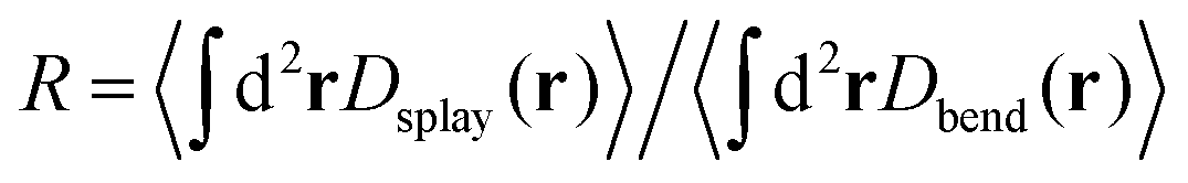. In equilibrium, equipartition requires that this ratio satisfy R_eq = k₃₃/k₁₁. In our simulations, we observe that R depends strongly on activity; however, the data for all parameter sets collapses when plotted as a function of the effective filament bend modulus κ_eff. This result is consistent with the concept of effective moduli, but shows that their values depend on activity.

To understand why the apparent modulus values depend on activity, we analyzed the power spectra associated with these strain energies (Fig. S4 in ref. 41). The power spectra exhibit two features: (1) Fig. 4B shows that for the smallest simulated effective rigidity, κ_eff = 2, the peak of the power spectrum k_peak is on the filament scale, indicating that most deformation energy arises due to bending of individual filaments. But for all higher values of κ_eff, a peak arises at the defect spacing scale, indicating that the defect density controls the texture in this active nematic. (2) Fig. 4C shows the magnitude of the power spectrum at the characteristic scale k_peak. The splay energy density is nearly independent of the effective filament stiffness, while the amount of bend decreases linearly with κ_eff for κ_eff ≲ κ^max_eff, where κ^max_eff ≈ 30 is the point at which the effective persistence length of the filaments is equal to their contour length. This observation demonstrates that energy injected into the system at the microscale due to activity preferentially dissipates into bend modes.

Defect shape

Let us now consider a striking feature of the texture of an active nematic, the shape of a defect. A quantitative descriptor of defect shape can be developed as follows. We choose a coordinate system with its origin at the center of the defect core, with the x-axis pointing along the defect orientation (see Fig. 5A). We work in polar coordinates, with r the radial distance from the defect core and ϕ as the azimuthal angle with respect to the x-axis. We define θ as the angle of the director field with respect to the x-axis. At any position, we can then express θ(r, ϕ) as a Fourier expansion in ϕ ∈ {−π:π}.However, in practice truncating the expansion after the first sin term approximates the shape of a defect well, so the descriptor simplifies to 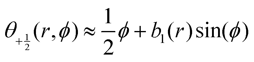, and the result is insensitive to r provided the measurement is performed outside of the defect core (see Fig. S10 (ESI†)⁴¹). Thus, the parameter b₁ uniquely describes the defect shape; in particular, larger values of b₁ correspond to pointier defects. Note that Zhang et al.¹² and Cortese et al.²² recently proposed similar approaches to characterizing defect shapes. An advantage of our approach is that the shape can be described by a single number, b₁.

Fig. 5B shows that the mode of b₁ calculated from defects within our simulations depends only on κ_eff, thus demonstrating that defect shape is controlled by the apparent bending rigidity. Moreover, b₁ increases logarithmically with κ_eff; i.e., defects become more pointed as the bending rigidity increases, consistent with the previous observations of highly pointed defects in rigid rod simulations.^2,35,52

Defect density

We next consider a well-studied property of an active nematic, the steady-state defect density.^19,24,28,53Fig. 6 shows that the defect density collapses onto a single curve when plotted as a function of κ_eff, and scales roughly as 1/κ_eff under parameter values for which the apparent persistence length lies between the monomer scale and filament contour length, 1.5 ≲ κ_eff ≲ κ^max_eff. We observe the same scaling for our other data set (Fig. S1, ESI†⁴¹). Hydrodynamic theories such as ref. 19, 24, 28 and 53 predict that the defect density scales as α/K, where α is the measure of active stress in the hydrodynamic theories and K is a Frank elastic constant. The scaling collapse observed in our simulations indicates that these hydrodynamic parameters are directly related to their microscopic analogs, namely the filament elastic constant κ and the collisional active stress ∼(1 + (f^a)²). Note that we could not measure defect densities in systems with both extremely high activity and high bare bending rigidity (f^a ≥ 20 and κ ≳ 5000) because our defect detection algorithm breaks down (see Section S8 of ref. 41).

Number fluctuations

Finally, previous work has shown that active nematics are susceptible to phase separation^36,54–56 and giant number fluctuations (GNFs).^5,54,57–59 We find that flexibility suppresses phase separation except at molecular scales (Fig. S8, ESI†⁴¹), but that number fluctuations are governed by the apparent modulus. We monitored number fluctuations by measuring the number of pseudoatoms within square subsystems with side lengths ranging from 20σ to 840σ. At equilibrium, in a region containing on average N particles the standard deviation of the number of particles ΔN scales as , while previous studies of active nematics have identified higher scaling, as large as ΔN ∼ N. Fig. S9 (ESI†)⁴¹ shows measured number fluctuations for different values of the effective bending modulus. We see that for small κ_eff = 2 the result is constant with subsystem size, indicating equilibrium-like fluctuations, but the slope increases for larger effective modulus values, indicating a progression toward GNFs. At all κ_eff the fluctuations are eventually suppressed on scales comparable to the defect spacing (N ≳ 10⁴), at which scale the system is essentially isotropic, consistent with Narayan et al.⁵

To determine the dependence on κ_eff, we fit the data for each simulation in the range N ≤ 10⁴ to the form aN^g, so that g = 0 indicates equilibrium-like fluctuations and g = 0.5 would indicate linear scaling of fluctuations with system size. As shown in Fig. 7, g increases with κ_eff, with g = 0 for small κ_eff and g ≈ 0.3 for the largest effective bending rigidity values investigated; i.e. ΔN ∼ N^0.8. The fact that g < 0.5 for the parameters we consider may reflect suppression of fluctuations even for N < 10⁴. Importantly, estimated values of g at different f^a and κ collapse onto a single function of κ_eff, consistent with the observations of the other characteristics of an active nematic shown above.

Comparison with equilibrium

For small values of κ_eff, the bend/splay ratio in our model active nematic roughly scales as R ∼κ^1/2_eff (Fig. 4). This differs from the scaling of an equilibrium nematic, where the moduli scale as k₃₃ ∼ κ and k₁₁ ∼ κ^1/3,^60,61 giving R_eq ∼ κ^2/3. We confirmed this scaling by calculating the equilibrium moduli for our system (Fig. S5, ESI†⁴¹) using the free energy perturbation technique of ref. 62. Analysis of simulation trajectories suggests that the difference in scaling arises because the active systems have much higher nematic order than the equilibrium systems (when compared at the same values of effective bending rigidity). In an equilibrium system, increasing the filament flexibility decreases order, resulting in a transition from the nematic to isotropic phase as κ decreases below 5 at the density used in our simulations.⁶³ In contrast, the active systems remain deep within the nematic phase (S ≳ 0.8) for all parameter sets (Fig. S5c in ref. 41). We empirically found that normalizing the bend–splay ratio by the degree of order, using the form R/S², roughly collapses the equilibrium and active results onto a single curve (Fig. S5b, ESI†⁴¹). Although we cannot rationalize the form of the normalization, this result implies that the differences in scaling between active and equilibrium cases arise from the increased nematic order in the active simulations.

Returning to the defect shape measurements, the dashed line in Fig. 5B shows the defect shape parameter values b₁ calculated by minimizing the continuum Frank free energy for an equilibrium system containing a separated pair of and defects. Here we have fixed the continuum modulus k₁₁ and varied k₃₃ so that matches the value obtained from our microscopic simulations at the corresponding value of effective stiffness: R_eq(k₃₃) = R(κ_eff). Although the equilibrium b₁ values are shifted above the simulation results, consistent with the discrepancy in R between the active and passive systems described above, we observe the same scaling with bending rigidity in the continuum and simulation results. Thus, the defect shape measurement provides a straightforward means to estimate effective moduli in simulations or experiments on active nematics.

IV. Conclusions

In active materials, energy injected at the particle scale undergoes an inverse cascade, manifesting in collective spatiotemporal dynamics at larger scales. The nature of this emergent behavior depends crucially on which modes the active energy dissipates into. Our simulations show that activity within a dry active nematic preferentially dissipates into bend modes, thus softening the apparent bend modulus. Consequently, the value of the apparent bend modulus depends strongly on activity. However, we show that once this dependence on activity is accounted for, this effective modulus dictates all collective behaviors that we investigated – the relative amounts of bend and splay, defect density, defect shape, and giant number fluctuations. The dependence of multiple characteristics on this single parameter suggests that material properties such as apparent moduli can be meaningfully assessed in an active nematic and related to their values at equilibrium, provided their dependence on activity is accounted for. Finally, our technique to parameterize defect shapes allows estimating the relative magnitudes of these effective moduli in any experimental or computational system that exhibits defects.

Experimental confirmation of the predicted dependence of effective bend and splay moduli on activity

After a preprint of our manuscript first appeared, ref. 64 presented elegant experimental results confirming that the ratio of apparent bend and splay moduli depend on activity as predicted here.

Conflicts of interest

There are no conflicts to declare.

Acknowledgements

This work was supported by the Brandeis Center for Bioinspired Soft Materials, an NSF MRSEC, DMR-1420382 (AJ, EP, AB, MFH) and NSF DMR-1149266 (AB). Computational resources were provided by NSF XSEDE computing resources (MCB090163, Stampede) and the Brandeis HPCC which is partially supported by DMR-1420382.

References

1. T. Sanchez, D. T. N. Chen, S. J. Decamp, M. Heymann and Z. Dogic, Nature, 2012, 491, 431–434.
2. S. J. DeCamp, G. S. Redner, A. Baskaran, M. F. Hagan and Z. Dogic, Nat. Mater., 2015, 14, 1110–1115.
3. C. Peng, T. Turiv, Y. Guo, Q.-H. Wei and O. D. Lavrentovich, Science, 2016, 354, 882–885.
4. S. Zhou, A. Sokolov, O. D. Lavrentovich and I. S. Aranson, Proc. Natl. Acad. Sci. U. S. A., 2014, 111, 1265–1270.
5. V. Narayan, S. Ramaswamy and N. Menon, Science, 2007, 317, 105–108.
6. V. Narayan, N. Menon and S. Ramaswamy, J. Stat. Mech.: Theory Exp., 2006, 2006, P01005.
7. G. Duclos, C. Erlenkämper, J.-F. Joanny and P. Silberzan, Nat. Phys., 2017, 13, 58.
8. D. J. Broer, Nat. Mater., 2010, 9, 99–100.
9. I.-h. Lin, D. S. Miller, P. J. Bertics, C. J. Murphy, J. J. de Pablo and N. L. Abbott, Science, 2011, 332, 1297–1300.
10. M. Kleman, Rep. Prog. Phys., 1989, 52, 555–654.
11. S. Zhou, S. V. Shiyanovskii, H.-S. Park and O. D. Lavrentovich, Nat. Commun., 2017, 8, 14974.
12. R. Zhang, N. Kumar, J. L. Ross, M. L. Gardel and J. J. de Pablo, Proc. Natl. Acad. Sci. U. S. A., 2018, 115, E124–E133.
13. F. C. Frank, Discuss. Faraday Soc., 1958, 25, 19.
14. C. W. Oseen, Trans. Faraday Soc., 1933, 29, 883–899.
15. R. A. Simha and S. Ramaswamy, Phys. Rev. Lett., 2002, 89, 058101.
16. M. C. Marchetti, J. F. Joanny, S. Ramaswamy, T. B. Liverpool, J. Prost, M. Rao and R. A. Simha, Rev. Mod. Phys., 2013, 85, 1143–1189.
17. S. Ramaswamy, Annu. Rev. Condens. Matter Phys., 2010, 1, 323–345.
18. L. Giomi, M. J. Bowick, X. Ma and M. C. Marchetti, Phys. Rev. Lett., 2013, 110, 228101.
19. L. Giomi, M. J. Bowick, P. Mishra, R. Sknepnek and M. Cristina Marchetti, Philos. Trans. R. Soc., A, 2014, 372, 20130365.
20. A. Doostmohammadi, T. N. Shendruk, K. Thijssen and J. M. Yeomans, Nat. Commun., 2017, 8, 15326.
21. A. U. Oza and J. Dunkel, New J. Phys., 2016, 18, 093006.
22. D. Cortese, J. Eggers and T. B. Liverpool, Phys. Rev. E, 2018, 97, 022704.
23. T. N. Shendruk, K. Thijssen, J. M. Yeomans and A. Doostmohammadi, Phys. Rev. E, 2018, 98, 010601.
24. S. P. Thampi, R. Golestanian and J. M. Yeomans, EPL, 2014, 105, 18001.
25. L. Giomi, Phys. Rev. X, 2015, 5, 031003.
26. L. M. Lemma, S. J. Decamp, Z. You, L. Giomi and Z. Dogic, arXiv preprint arXiv:1809.06938, 2018.
27. T. N. Shendruk, A. Doostmohammadi, K. Thijssen and J. M. Yeomans, Soft Matter, 2017, 13, 3853–3862.
28. M. M. Norton, A. Baskaran, A. Opathalage, B. Langeslay, S. Fraden, A. Baskaran and M. F. Hagan, Phys. Rev. E, 2018, 97, 012702.
29. T. Gao, M. D. Betterton, A.-S. Jhang and M. J. Shelley, Phys. Rev. Fluids, 2017, 2, 093302.
30. P. Guillamat, J. Ignés-Mullol and F. Sagués, Nat. Commun., 2017, 8, 564.
31. F. C. Keber, E. Loiseau, T. Sanchez, S. J. DeCamp, L. Giomi, M. J. Bowick, M. C. Marchetti, Z. Dogic and A. R. Bausch, Science, 2014, 345, 1135–1139.
32. R. Zhang, Y. Zhou, M. Rahimi and J. J. De Pablo, Nat. Commun., 2016, 7, 13483.
33. P. W. Ellis, D. J. G. Pearce, Y.-W. Chang, G. Goldsztein, L. Giomi and A. Fernandez-Nieves, Nat. Phys., 2017, 14, 85.
34. F. Alaimo, C. Köhler and A. Voigt, Sci. Rep., 2017, 7, 5211.
35. T. Gao, R. Blackwell, M. A. Glaser, M. D. Betterton and M. J. Shelley, Phys. Rev. Lett., 2015, 114, 048101.
36. X.-q. Shi and Y.-q. Ma, Nat. Commun., 2013, 4, 3013.
37. S. Henkes, M. C. Marchetti and R. Sknepnek, Phys. Rev. E, 2018, 97, 042605.
38. Y. Sumino, K. H. Nagai, Y. Shitaka, D. Tanaka, K. Yoshikawa, H. Chaté and K. Oiwa, Nature, 2012, 483, 448.
39. P. Guillamat, J. Ignés-Mullol and F. Sagués, Proc. Natl. Acad. Sci. U. S. A., 2016, 113, 5498–5502.
40. Image provided by Linnea Metcalf, Achini Opathalage and Zvonimir Dogc and used with their permission.
41. ESI† to this paper is provided at DOI: 10.1039/c8sm02202j.
42. S. Plimpton, J. Comput. Phys., 1995, 117, 1–19.
43. K. R. Prathyusha, S. Henkes and R. Sknepnek, Phys. Rev. E, 2018, 97, 022606.
44. J. D. Weeks, D. Chandler and H. C. Andersen, J. Chem. Phys., 1971, 54, 5237–5247.
45. K. Kremer and G. S. Grest, J. Chem. Phys., 1990, 92, 5057–5086.
46. F. Peruani, A. Deutsch and M. Bär, Phys. Rev. E: Stat., Nonlinear, Soft Matter Phys., 2006, 74, 030904.
47. S. R. McCandlish, A. Baskaran and M. F. Hagan, Soft Matter, 2012, 8, 2527–2534.
48. S. Weitz, A. Deutsch and F. Peruani, Phys. Rev. E: Stat., Nonlinear, Soft Matter Phys., 2015, 92, 012322.
49. F. Ginelli, F. Peruani, M. Bär and H. Chaté, Phys. Rev. Lett., 2010, 104, 184502.
50. F. Peruani, J. Starruß, V. Jakovljevic, L. Søgaard-Andersen, A. Deutsch and M. Bär, Phys. Rev. Lett., 2012, 108, 098102.
51. A. Baskaran and M. C. Marchetti, Phys. Rev. Lett., 2008, 101, 268101.
52. X.-q. Shi, H. Chaté and Y.-q. Ma, New J. Phys., 2014, 16, 035003.
53. E. Putzig, G. S. Redner, A. Baskaran and A. Baskaran, Soft Matter, 2015, 12, 1–5.
54. S. Mishra and S. Ramaswamy, Phys. Rev. Lett., 2006, 97, 090602.
55. S. Ngo, A. Peshkov, I. S. Aranson, E. Bertin, F. Ginelli and H. Chaté, Phys. Rev. Lett., 2014, 113, 038302.
56. E. Putzig and A. Baskaran, Phys. Rev. E: Stat., Nonlinear, Soft Matter Phys., 2014, 90, 042304.
57. S. Ramaswamy, R. A. Simha and J. Toner, Europhys. Lett., 2003, 62, 196–202.
58. H. Chaté, F. Ginelli and R. Montagne, Phys. Rev. Lett., 2006, 96, 180602.
59. H. P. Zhang, A. Be'er, E.-L. Florin and H. L. Swinney, Proc. Natl. Acad. Sci. U. S. A., 2010, 107, 13626–13630.
60. J. V. Selinger and R. F. Bruinsma, Phys. Rev. A: At., Mol., Opt. Phys., 1991, 43, 2910–2921.
61. M. Dijkstra and D. Frenkel, Phys. Rev. E: Stat. Phys., Plasmas, Fluids, Relat. Interdiscip. Top., 1995, 51, 5891–5898.
62. A. A. Joshi, J. K. Whitmer, O. Guzmán, N. L. Abbott and J. J. de Pablo, Soft Matter, 2014, 10, 882–893.
63. Note that this 2D system with soft-core interactions should exhibit quasi-long-range order in the nematic phase,^65–67 and thus S decays with system size. Since we are interested in the degree of order on the scale of typical bend and splay fluctuations, we report S values measured within regions of size 10 × 10σ² (see ref. 41).
64. N. Kumar, R. Zhang, J. J. de Pablo and M. L. Gardel, Sci. Adv., 2018, 4, eaat7779.
65. J. P. Straley, Phys. Rev. A: At., Mol., Opt. Phys., 1971, 4, 675–681.
66. D. Frenkel and R. Eppenga, Phys. Rev. A: At., Mol., Opt. Phys., 1985, 31, 1776–1787.
67. J. M. Kosterlitz and D. J. Thouless, J. Phys. C: Solid State Phys., 1973, 6, 1181.

---

Footnote

† Electronic supplementary information (ESI) available. See DOI: 10.1039/c8sm02202j

---