Dissolved organic matter in urban stormwater runoff at three typical regions in Beijing: chemical composition, structural characterization and source identification

Abstract

In this work, DOM was extracted from urban stormwater runoff samples collected at three typical regions (business, residential and campus regions) in Beijing, China. A comparison between the chemical characteristics of DOM extracted from these three regions was performed using UV-visible spectrometry (UV-vis), excitation–emission matrix (EEM) fluorescence, proton nuclear magnetic resonance spectroscopy (¹H NMR) and ultra-performance liquid chromatography quadrupole time-of-flight mass spectrometry (UHPLC-Q-TOF-MS). The UV-vis and EEM spectra revealed that the DOM in stormwater runoff samples mainly contained UV humic-like (peak A) compositions with higher molecular weights. ¹H NMR analysis indicated that the DOM of the three regions contained a similar distribution of functional groups, which mainly consisted of aliphatic chains and aromatic components with carbonyl, hydroxyl or alkyl terminal groups. And the UHPLC-Q-TOF-MS demonstrated the identification and characterization of possible compounds existing in the DOM. Further studies should focus on the interactive relationship between DOM and the co-existing contaminants (heavy metals and some typical organic pollutants) in stormwater runoff.

---

1. Introduction

Stormwater runoff has been confirmed as one of the major sources of pollutants threatening the quality of receiving waters,^1–3 considering that stormwater can flush and further dissolve a large amount of pollutants from upstream impervious area.^4–7 Previous studies have paid more attention to some conventional parameters of stormwater runoff, like biochemical oxygen demand (BOD), chemical oxygen demand (COD), total suspended solid (TSS), total nitrogen (TN), nitrate–nitrogen (NO₃–N), orthophosphorus (PO₄–P), total phosphorus (TP) and heavy metals.^1–3,8–11 However, up to now, nearly nothing is known about the nature and role of dissolved organic matter (DOM) in urban stormwater runoff, except that McElmurry and coworkers opened a door of this field, in which the influence of land cover and environmental factors on the DOM in stormwater runoff were presented.¹²

DOM, being operationally defined as the fraction which can pass through a 0.45 μm membrane,¹³ is a heterogeneous mixture of aromatic and aliphatic organic compounds, including but not limited to proteins, carbohydrates, polysaccharides, lipids and humus.¹⁴ In terrestrial and aquatic ecosystems, DOM plays a crucial role on the geochemical and photochemical reactions by participating in carbon (C) and nutrient (N, P, and S) cycles. Also, DOM dominates microbially mediated reactions via serving as potential substrate,¹⁵ in which it is the base of the food web, providing energy to heterotrophic organisms and further controlling biological processes, like microbial degradation.^12,16–18 Furthermore, DOM can strongly interact with organic and inorganic contaminants, as well as heavily influencing their transport, transformation, bioavailability, toxicity and ultimate fate.^19–27 Therefore, DOM is very important in various biochemical and physical processes linking terrestrial and aquatic ecosystems. In the last decades, a large amount of researches on DOM and its interactions with coexistences in soil, aquatic ecosystems (including water and sediment), and even in stormwater, were conducted, with the aid of a diverse array of analytical chemical methods, like UV-visible spectroscopy (UV-vis),^12,28–31 excitation–emission matrix spectroscopy (EEMs),^28–34 proton nuclear magnetic resonance spectroscopy (¹H NMR)^{28–31,35,36} and quadrupole time-of-flight mass spectrometer (Q-TOF-MS).^37–40 McElmurry et al.¹² and Taylor et al.⁴¹ explored the compositions of DOM in stormwater runoff from suburban and urban sources, considering the influence of major environmental factors on the DOM and its impacts on receiving waters. But up to now, few researches were carried out on the nature, properties, possible structure of DOM, to say nothing of its interactions with coexisting pollutants in urban stormwater runoff, which is assumed to act as important intermediate between natural stormwater, terrestrial and aquatic ecosystems. In this work, the DOM in urban stormwater runoff collected at three typical regions in Beijing were characterized and investigated via UV-vis, EEMs, ¹H NMR and UHPLC-Q-TOF-MS to clarify the chemical composition, structural characterization and sources.

2. Materials and methods

2.1. Stormwater runoff sampling and sample preparation

Urban stormwater runoff samples were collected on 29^th July, 2014, at three sampling regions, which were Beijing Zoo business circle (39°56′ N, 116°20′ E), Dongluoyuan residential area close to the southern 3^rd ring road of Beijing (39°51′ N, 116°24′ E) and new campus (Daxing District) of Beijing University of Civil Engineering and Architecture (39°44′ N, 116°17′ E), respectively (as illustrated in Fig. 1). Meteorological data including rainfall, rain duration, surface temperature, relative humidity, pressure and watershed area were also recorded, as described in Table 1. All the underlying surface material of these three regions is asphalt pavement,^42–44 which facilitate to study the chemical features and spatial variation of DOM in stormwater runoff with identical land cover.

Fig. 1 Map of location of the three sampling regions.

Table 1 The meteorological data of all the regions

	Business	Campus	Residential
Rain amounts (mm)	30.8	31.6	32.4
Rain duration (min)	180	110	178
Relative humidity (%)	94	90	92
Pressure (in mmHg)	29.42	29.28	29.35
Watershed area (m^2)	256	112	855
Surface temperature (°C)	23	21	22

---

At each sampling site, the 13 individual samples were collected into glass bottles (600 mL) with glass funnel (30 cm diameter) under the sewer grate which was opened in advance, at the time of 0, 3, 6, 9, 14, 19, 24, 34, 44, 59, 74, 89, 119 min, after the start (being defined as t = 0 min) of runoff events.¹² Each sample was labeled by the sampling sequence of the corresponding regions (B#, C# and R#), where B, C and R represented business, campus and residential area, respectively, and # corresponded to the sample number. Prior to sampling, all glass materials were soaked for 30 min in a solution of NaOH (0.1 M), then washed by distilled water, followed by another immersion for 24 h in a solution of HNO₃ (4 M), and finally rinsed with ultrapure (Milli-Q) water. After collection, the samples were filtered through hydrophilic PVDF Millipore membrane filters (0.45 μm) and tested as soon as possible. Otherwise, the remaining samples should be stored in the dark at 4 °C for a maximum of 4 d, which was demonstrated the optimum for keeping the optical properties of the samples unchanged. All samples were required to reach room temperature to the subsequent analysis.^28,30,31,45

2.2. Dissolved organic carbon (DOC)

The DOC contents of the samples were theoretically calculated as the difference TC–TIC.^30,31 The concentrations of total carbon (TC) and total inorganic carbon (TIC) of each sample were determined by a Jena multi N/C 3100 analyzer (Germany). In order to conduct TIC measurements, standards were performed from 3.5000 g sodium hydrogen carbonate (reagents grade) plus 4.4163 g sodium carbonate (reagents grade) in 1000 mL ultrapure water, then the solution diluted to the concentration of 1, 5, 10, 20, 30, 40, 50 mg C L⁻¹. To carry out TC quantification, standards were prepared from 2.1254 g potassium hydrogen phthalate (reagents grade) plus 3.5000 g sodium hydrogen carbonate (reagents grade) and 4.4163 g sodium carbonate (reagents grade) dissolved in 1000 mL ultrapure water, then the mixed solutions were diluted to the concentration of 2, 10, 20, 40, 60, 80, 100 mg C L⁻¹. Control standards were generally within ±5% agreement in terms of TC and TIC content. For each sample, three replicates were analyzed to determine the TC and TIC contents to ensure the relatively precise TOC values.^30,31

2.3. UV-visible spectroscopy

Due to the DOM content of runoff samples in this study was much higher than in stormwater, 1 cm rather than 10 cm quartz cells, were selected to conduct the UV-visible analysis.^30,31,46 And the UV-visible spectra in the range of 240–400 nm were recorded on a Perkin-Elmer lambda 650S spectrophotometer (America). Highly absorbing samples were diluted with ultrapure water (Milli-Q) to the point where absorbance at 300 nm was ≤0.02 to minimize inner filter effect.⁴⁷ Ultrapure water was used to run blanks.

2.4. Excitation–emission matrix (EEM) fluorescence spectroscopy

Fluorescence measurements of DOM in the urban stormwater runoff were conducted on a Hitachi F-7000 fluorescence spectrophotometer (Japan) equipped with a xenon flash lamp, using 1 cm quartz cells. The emission wavelengths (E_m, nm) scans from 200 to 550 nm, at excitation wavelengths (E_x, nm) from 200 to 550 nm every 5 nm, with a 10 nm slit width, a PMT voltage of 700 V and scanning speed of 1200 nm min⁻¹. Quinine sulfate in 0.1 N H₂SO₄ was selected as the reference standard with its minimum detection limit of 0.4 ppb in this fluorescence spectrophotometer.⁴⁸ The relative fluorescent intensities of the samples can be expressed in terms of standard quinine sulfate units (QSU), saying that 55.5 intensity units equal to one QSU (1 QSU = 1 ppb quinine sulfate in 0.05 mol L⁻¹ H₂SO₄),^32,49–52 which permits inter-laboratory comparisons. Furthermore, removing Raman and Rayleigh scattering is also important to avoid interference in data interpretation caused by the intense noises. In this study, Rayleigh scatter was removed from the data set by adding zero to the EEMs in the two triangle regions (E_m ≤ E_x + 20 nm and ≥2E_x − 10 nm),⁵³ and Raman scatter were eliminated from all spectra by subtracting the ultrapure water blank spectra.³⁰ The resulting map represents a specific fingerprint of the DOM in the urban stormwater runoff samples.

2.5. ¹H NMR spectroscopy

Prior to the ¹H NMR spectroscopy analysis, DOM is isolated and extracted from 100 mL runoff samples filtered through hydrophilic PVDF Millipore membrane filters (0.45 μm) using Agilent Vac Elut SPS 24 solid phase extraction (SPE) equipment (California, America) with Bond Elut C-18 as sorbent. Before extraction, C-18 cartridges were conditioned by washing twice with 5 mL of a 10% water in methanol solution, followed by two 5 mL water aliquots. Throughout this study, ultrapure water (18.2 MΩ cm⁻¹) was used for reagents preparation and washing. Filtered samples were extracted by drawing 100 mL through the C-18 cartridge at a flow of 2 mL min⁻¹. Two 5 mL aliquots of ultrapure water were passed through the cartridges after the stormwater runoff sample to remove residual salts. The samples were then eluted off the C-18 cartridges with 6 mL aliquots of 10% water in methanol, followed by continuous running under reduced pressure for 30 min to remove solvent from C-18 cartridges completely.⁴⁵ The samples were transferred to 15 mL glass vials, and dried under nitrogen atmosphere by Termovap Sample Concentrator (YGC-1217, Baojing Company).³¹

For ¹H NMR analysis, the solid extracts of the samples were dissolved in D₂O (Jin Ouxiang Company). The ¹H NMR spectra were recorded on an Agilent 500M DD2 NMR spectrometer with an operating frequency of 499.898 MHz. The acquisition of spectra was performed with a contact time of 2.045 s and with the standard s2pul pulse sequence. The recycle delay was 1 s and the length of the proton 90° pulses was 10.8 μs. About 256 scans were collected for each spectrum. A 1.0 Hz line broadening weighting function and baseline correction was applied. The identification of functional groups in the NMR spectra was based on their chemical shift (δ_H) relative to that of the water (4.7 ppm).³¹

2.6. Ultra-performance liquid chromatography quadrupole time-of-flight mass spectroscopy

A Bruker Daltonics impact HD UHR-Q-TOF-MS (Bremen, Germany) equipped with an electrospray ionization source (ESI), which was coupled with UHPLC system (Agilent 1290), was introduced to carry out the chemical characterization of the DOM in urban stormwater runoff (mass resolving power ≥ 50 000) at molecular level. Prior to analysis, 15 mL samples of B1, C1 and R1 were filtrated via hydrophilic PVDF Millipore membrane (0.45 μm). The analytes were separated by a Thermo Acclaim RSLC 120 C-18 column (2.2 μm, 120 Å, 2.1 × 100 mm) on an Agilent 1290 UHPLC equipped with a DAD detector. Acidified water (0.1% formic acid, v/v) and acidified acetonitrile (0.1% formic acid, v/v) were used as mobile phases A and B, respectively.³⁸ Gradient was programmed as the following: 0 min, 2% B; 2 min, 2% B; 5 min, 5% B; 25 min, 95% B; 30 min, 95% B, and finally, the initial condition was held for 5 min as a re-equilibration step. The flow rate was set at 0.3 mL min⁻¹ throughout the gradient. The column temperature was maintained at 30 °C, and the injection volume was 20 μL, meanwhile, ultrapure water (Milli-Q) was used to carry out blank.

Mass detection was operated in both positive ionization and negative ionization modes with parameters as the following: capillary, +4500 V; nebulizing gas pressure, 1.8 bar, drying gas (N₂) flow, 9.0 L min⁻¹; dry gas temperature, 200 °C; collision RF, 150 V_pp; transfer time 70 μs, and pre-pulse storage, 5 μs. The UHPLC/MS accurate mass spectra were recorded across m/z range from 50 to 1100, calibrated by external standard sodium formate. The MS data were processed through Data Analysis 4.0 software (Bruker Daltonics, Bremen, Germany), which provided a list of possible elemental formulas by using the Smart Formula™ editor (mass accuracy ≤ 10 ppm). The editor uses a CHNO algorithm, which provides standard functionalities such as minimum/maximum elemental range, electron configuration, and ring-plus double bond equivalents, as well as a sophisticated comparison of the theoretical with the measured isotope pattern (mSigma value) for increasing the confidence in the suggested molecular formula.^54,55

3. Results and discussion

3.1. UV-visible spectroscopy

The UV-visible spectra obtained for the runoff samples of three regions are shown in Fig. 2. For all samples, the decrease in absorbance with wavelength follows a trend similar to that already observed for natural stormwater samples.^28,30,56 The spectra of the samples show a very small shoulder in the region of 250–300 nm, which is usually attributed to π → π* electron transitions of unsaturated systems.⁵⁷

Fig. 2 UV-visible spectrum of the stormwater runoff samples of three regions: (a) business; (b) residential; (c) campus.

In order to clarify the nature of the DOM chromophores and get information about the molecular weight of DOM, the spectral slope coefficient (S, μm⁻¹), being a parameter inferred from UV-visible spectra, was introduced to demonstrate how efficiently DOM absorbs light as a function of the wavelength.⁵⁸ S can be calculated from non-linear least-square regressions of the absorption coefficients a(λ) vs. wavelength ranging from 240 to 400 nm, as listed in eqn (1) and (2):

a_λ = a_λ0e^{S(λ₀−λ)} + K (1)

a_λ = 2.303A_λ/l (2)

where, a_λ is absorption coefficients, A_λ is the absorbance at wavelength λ (nm), l (m) is the optical path length (l = 0.01 m in this study), a_λ0 is the absorption coefficients at reference wavelength, λ₀ is the reference wavelength (300 nm was selected in this study), λ is the selected wavelength (ranging 240 to 400 nm), K is a background parameter to improve the goodness of fitting.

The S values of DOM in urban stormwater runoff samples of three regions (business, residential and campus) were in the range of 13.22–17.94, 15.43–19.68 and 7.99–16.3 μm⁻¹, with median values of 14.59, 16.71 and 13.64 μm⁻¹ for business, residential and campus, respectively, which were similar to the study results of the DOM of stormwater reported by Miller and co-workers²⁹ (average value 18.9 μm⁻¹). Additionally, the changes of S values of DOM during three storm events were also investigated (Fig. S1, ESI†). The results revealed that the S values of three regions reached the peak in the first 10 min, and then reduced gradually to a relatively stable level. Previous studies had suggested an inverse relationship of DOM molecular weight with the value of S,^59,60 so the results implied that the molecular weight of DOM became larger in the later stage of storm events.

To assess the aromaticity of DOM in the runoff samples, specific ultraviolet absorbance at 280 nm (SUVA₂₈₀) rather than SUVA₂₅₄ was introduced, due to (1) the transfer of electrons between overlapping π-orbitals occurs at 280 nm for conjugated systems, such as those in aromatic molecules and other humic like organic substances, and (2) the presence of other dissolved species (like nitrate, iron ions), which also absorb UV light, and can be ubiquitous in natural waters, but can't absorb UV light at 280 nm.^12,61–63 SUVA₂₈₀ was calculated by dividing the amount of UV light absorbed at 280 nm by the concentration of DOC,^63,64 and positively correlated to DOM aromaticity.^61,65

The median values of SUVA₂₈₀ were 1.85, 2.37 and 3.59 L mg C⁻¹ m⁻¹ for business, campus and residential regions, respectively, revealing that a greater amount of aromatic structures present in the organic substances.¹² In addition, the SUVA₂₈₀ values increased with the storm event (Fig. S2, ESI†), implying more and more aromatic structures arise in later stormwater runoff. The vehicle exhaust,⁶⁶ asphalt pavement precipitates,^67–69 landfill leachate,⁷⁰ and atmospheric polycyclic aromatic hydrocarbons^71–73 washed by the wet precipitation could be the possible sources of aromatic substances of stormwater runoff.

Kieber and co-workers²⁸ have demonstrated that a(300), i.e. absorbance coefficient at 300 nm, can be applied as an index of chromophoric DOM abundance. In this study, a(300) ranged from 24.87 to 303.99, 46.52 to 146.93 and 77.38 to 654.97 m⁻¹ for business, campus and residential area, respectively. Considering the DOC concentrations ranging from 553.33 to 8320.83, 558.33 to 3988.33 and 2483.33 to 7619.17 μM C, respectively, there was a significant positive correlation between a(300) and DOC concentrations, as illustrated in Fig. 3. It was deduced that chromophoric DOM was an important and ubiquitous contributor to the dissolved organic carbon pool in stormwater runoff.²⁸

Fig. 3 Absorbance coefficient at 300 nm (m⁻¹) versus DOC concentration (μM C): (a) business, r² = 0.97; (b) residential, r² = 0.74; (c) campus, r² = 0.98.

3.2. Excitation–emission matrix (EEM) fluorescence spectroscopy

Excitation–emission matrix (EEM) fluorescence spectroscopy was suggested to be powerful tool to distinguish DOM types, which could determine the specific fluorescent fractions in organic matters from different sources with much higher sensitivity.^28,49 EEM can identify humic-like (designated as A, C and M) and protein-like fluorescence peaks (B and T), as listed in Table 2, using excitation–emission wavelength pairs of fluorescent peaks.⁴⁹ All runoff samples in this study were characterized by EEM to gain insight into the structure nature of the chromophoric DOM. All the spectra of the three regions were depicted in Fig. 4–6. It is obvious that the peak A occurred alone in the EEM spectra for all samples collected from three typical regions (business, residential and campus), indicating that UV humic-like compounds are the major fluorophores components in the DOM of all runoff samples. And the corresponding fluorescence intensities of DOM three regions for peak A varied from 118 to 1216, 483 to 3533 and 65 to 600 quinine sulfate units (QSU), respectively. No significant signals of peak C (visible humic-like, more aromatic substances), peak B (tyrosine-like substances) and peak T (protein like tryptophan), were identified from the EEM spectra in this study.

Table 2 Peaks, description and excitation/emission maxima of fluorescent DOM

Peaks	Description	Excitation max (nm)	Emission max (nm)
A	UV humic-like, less aromatic	<260	380–460
C	Visible humic-like, more aromatic	320–360	420–460
M	Marine-humic like	290–310	370–410
B	Tyrosine-like substances	260	280
T	Protein-like tryptophan	250–300	305–355

---

Fig. 4 EEM fluorescence contour profiles of business region. (a)–(m) Corresponded to the samples collected at the time 0–119 min.

Fig. 5 EEM fluorescence contour profiles of campus region. (a)–(m) Corresponded to the samples collected at the time 0–119 min.

Fig. 6 EEM fluorescence contour profiles of residential region, (a)–(m) corresponded to the samples collected at the time 0–119 min.

The differences in fluorescence properties of the DOM from three regions were further assessed by determining three indices, namely the fluorescence index (FI),^74–76 the humification index (HIX)^33,77,78 and the biological index (BIX).^33,76,78 FI is defined as the ratio of fluorescence intensity at the emission wavelength 450 nm to that at 500 nm at the excitation wavelength 370 nm. HIX is the ratio H/L of two spectral region areas from the emission spectrum scanned for an excitation at 254 nm. The two areas are calculated between emission wavelengths 300 and 345 nm for L and between 435 and 480 nm for H. And BIX is calculated at excitation 310 nm, by dividing the fluorescence intensity emitted at the emission wavelength 380 nm and 430 nm.

The FI, HIX and BIX values of the runoff samples in three regions are listed in Table 3. The fluorescence index can be used to potentially discriminate the source of DOM,⁷⁴ and our FI values (1.24–1.65) were in the range of 1.4–1.9, suggesting that the sources of DOM in the runoff samples were consistent with predominantly terrestrial sources, or both terrestrial and microbial sources.⁷⁵ When the degree of aromaticity of DOM increases, red-shift occurred in the emission spectrum, implying that the ratio H/L, and thus HIX, increases.⁷⁶ The HIX is usually used to estimate the degree of maturation (aromaticity) of DOM.^33,77 The ranges of HIX values of DOM in our study were 1.72–9.21, 3.49–22.86 and 1.86–5.38 for business, residential and campus regions, respectively. The HIX values of DOM for the samples collected from residential region demonstrated that the degree of maturation of residential samples was much higher than that of the other two regions. All the HIX values in this study implied that the DOM was both autochthonous and allochthonous organic materials.⁷⁸ The BIX can provide information about the organic matter source, which can reflect autochthonous biological activities.^33,78 High BIX values (>1) correspond to a biological origin, and low values (<1) imply low abundance of organic matter of biological origin.^33,78 BIX values of the runoff samples in this study varied from 0.54 to 1.04, 0.57 to 0.88 and 0.68 to 0.86 for the business, residential and campus region, respectively, indicating that most of organic substances were terrestrial sources, and lower DOM production from biological processes in stormwater runoff.^33,78

Table 3 Fluorescence indices for stormwater runoff at three regions

Region	FI	HIX	BIX
Business	1.32–1.53	1.72–9.21	0.54–1.04
Residential	1.24–1.65	3.49–22.86	0.57–0.88
Campus	1.41–1.56	1.86–5.38	0.68–0.86

---

3.3. ¹H NMR spectroscopy

Proton NMR spectroscopy (¹H NMR) was successfully introduced to characterize the natural organic matters (NOM) of wet precipitation.^28–30,45 Comparing to UV-visible and fluorescence spectroscopy, ¹H NMR can be used to determine structural moieties in the isolated DOM mixture, and to conduct straightforward quantitative analysis, due to the integrated area of the spectra being proportional to the moles of protons present in the samples. In this study, only the first samples, namely B1, C1 and R1, were selected as the representatives to carry out ¹H NMR detections, and the spectra of extracted DOM of the three samples are illustrated in Fig. 7(a). The spectra exhibit that some distinct peaks are overlaid by some much broader bands, implying the existence of complex mixtures of structures in the DOM. Although there were large variety of overlapping resonances, each ¹H NMR spectrum was investigated on the basis of the chemical shift assignments described in the literatures for stormwater DOM.^35,79 The signals at δ_H = 0.6–1.8 ppm can be assigned to the aliphatic protons (H–C). The regions of δ_H = 1.8–2.6 and 2.8–3.2 ppm implies the presence of aliphatic protons in α position to carbonyl groups or unsaturated carbon atoms (H–C–C=). And the signals of δ_H = 3.2–4.1 ppm and δ_H = 6.5–8.5 ppm can be designated to aliphatic protons on carbon atoms singly bound to oxygen atoms (H–C–O) and aromatic protons, respectively.

Fig. 7 (a) ¹H NMR spectra of extracted samples: residential, campus and business regions. The peak at 4.7 ppm indicates the water signal; (b) relative abundance of each type of protons, estimated as the partial integrals of the spectra reported in (a).

The distribution of the different types of protons estimated from the partial integrals of the observed ¹H NMR regions for each sample was illustrated in Fig. 7(b), implying that the extracted DOM from the samples of three regions exhibit quite similar patterns in terms of structural characteristics. Signals assigned to terminal methyl hydrogens H₃C–C (δ_H ≈ 0.9 ppm) and to polymethylene chains (CH₂)_n (δ_H ≈ 1.3 ppm) can be found in all the three spectra. Overall, protons in the saturated aliphatic structures were found to be dominant moieties (36–40%) for all three DOM samples, suggesting predominance of aliphatic moieties.^28,30,31,45

In the regions of δ_H = 1.8–2.6 and 2.8–3.2 ppm, the most prominent signals in the spectra of Fig. 7(a) arose from aliphatic protons linked to carbon atoms adjacent to C=C (including aromatic rings) or C=O double bonds,^30,31 which accounts for 24–25% of the total integrated area of the spectra. And δ_H = 3.2–4.1 ppm region accounts for 16–18% of the total integral of the spectra, indicating the presence of the functional groups of hydroxyl groups of polyols.^30,31 Particularly, the content of the aromatic protons (19–22%), reflected by very broad band of δ_H = 6.5–8.5 ppm in this study are higher than the former researches.^28,30,31 The aromatic rings containing electron withdrawing groups, such as carbonyl, carboxyl or nitro groups, were also proposed to interpret the aromatic signals present in spectra of water soluble organic carbon (WSOC).^79–81 As stated above, gasoline,⁶⁶ landfill leachate,⁷⁰ asphalt pavement precipitates,^67–69 atmospheric polycyclic aromatic hydrocarbons,^71–73 and etc. may be ascertained as the possible main sources of these species in DOM of stormwater runoff.

3.4. Ultra-performance liquid chromatography quadrupole time-of-flight mass spectroscopy

Q-TOF-MS is a kind of electrospray ionization mass spectrometer, which is a soft ionization technique that has become an important technique for identification and characterization of natural organic mixtures at molecular level.^82–85 In this study, only B1, C1 and R1, the first sample in each region, were selected to carry out Q-TOF-MS analysis. DOM molecules were separated by Agilent 1290 UHPLC, as illustrated in Fig. 8(a)–(h), and each sample was analyzed using six replicate injections in both ESI-positive and ESI-negative ionization modes to establish a strong statistical basis for interpreting the mass-to-charge ratio (m/z) and ion abundance generated by the mass spectrometer in the range of 50–1100 amu. A total of 12 247 m/z and 4776 m/z values were found in ESI-positive ionization mode and ESI-negative ionization mode, respectively.

Fig. 8 Total ions chromatogram for the three regions samples and blank: (a) and (b) B1 – ESI positive, negative mode; (c) and (d) R1 – ESI positive, negative mode; (e) and (f) C1 – ESI positive, negative mode; (g) and (h) blank – ESI positive, negative mode.

A large quantity of signals were obtained from the mass spectra, but it is difficult and pointless to identify all of them. Only the signals with the peak intensity ≥ 10 000 CPS based on accurate MS and MS/MS fragments were considered in this study. Taking the liquid chromatography retention time of 7.7 min as an example, both the ESI-positive and ESI-negative ionization modes signals were distinct and intense (Fig. 9(a) and (b)), which were mainly the [M + H]⁺ ion with an m/z of 206.0451 and [M − H]⁻ ion with an m/z of 204.0296. Being analyzed by using the Smart Formula™ editor and searching in compound databases (such as http://metlin.scripps.edu and http://www.chemspider.com, etc.), the molecular formula was C₁₀H₇NO₄, and the possible structures were depicted in Fig. 9(a) and (b), which was further confirmed by MS/MS signals corresponding to the substances after removing CO and H₂O in sequence, as depicted in Fig. 9(c) and (d).

Fig. 9 Positive and negative ionization modes Q-TOF mass spectra of DOM collected from the business region.

Furthermore, the compounds were further categorized in the van Krevelen diagrams (as illustrated in Fig. 10), which has been applied widely in the geochemistry studies.^86,87 Particularly, Mead et al.⁸⁸ used this method to explore the compositions and structures of DOM in continental and coastal stormwater. The van Krevelen diagram is constituted using the formula information (i.e., H/C and O/C ratios) to create plots showing the major biogeochemical classes of compounds, such as lipids, proteins, carbohydrates, lignin-like compounds, etc., in which the types of compounds can be conservatively assessed from the location of points in the van Krevelen plot.⁸⁹

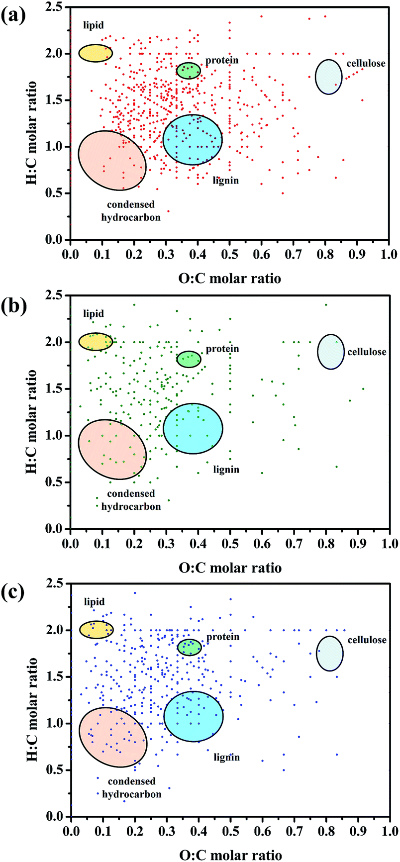Fig. 10 van Krevelen plots of the stormwater runoff samples of three regions: (a) business; (b) campus; (c) residential.

As shown in the Fig. 10, five types of compounds were identified, which were lipid, protein, cellulose, lignin and condensed hydrocarbon substances. However, the amounts of points suggested that lignin and condensed hydrocarbon substances were the dominated components in the three samples. The major structural categories of protons found in the NMR spectra were aliphatic and aromatic substances with carbonyl, carboxyl and hydroxyl functional groups, which could be an important part of the lignin and condensed hydrocarbon molecules.⁸⁶ Furthermore, as lignin has been widely considered to be a major portion of humic substances,⁹⁰ the results of van Krevelen plots further certified the accuracy of EEM fluorescence spectra.

In order to further understand the structures of entire compounds, which were speculated by retention time match between the observed peaks, compounds databases, as well as MS/MS experiments. All the compounds information of the three samples (retention time, intensity, maximum m/z, maximum molecular weight, formula, possible name, CAS, etc.) were listed in Tables S1–S6 (ESI†). The authentic standards of all compounds in this study failed to be conducted, since there were numerous m/z ions detected in the three samples. But through the compounds databases, the whole organic substances could be roughly divided into hydrophilic, amphiphilic and hydrophobic fractions. The hydrophilic fractions might include aromatic acids, fatty acids, hydroxyl compounds, and peptide-type and glucoside-type compounds, such as benzoic acid, butyric acid, Ile Lys Lys Tyr, 2,3-butanediol glucoside and diethylene glycol; the hydrophobic ones could present as indoles and carbonyl compounds, alkaloids and pesticides, such as 4-formyl indole, 2-octanone, eseroline and binapacryl; while lipid-type substances might be representatives of amphiphilic fractions.³⁸

As previously mentioned, the UHPLC-Q-TOF-MS technique can provide a novel method to trace the DOM source at the molecular level. In this study, DOM collected from the three typical regions might contained two primary sources as naturally autochthonous source, which was derived from biogenic sources types, e.g., plants and their metabolites during their biogeochemical process.^91,92 and allochthonous source, which originated from automobile exhaust, tobacco smoke, coal combustion and garbage leachate.^93,94

It is well known that DOM has hydrophilic and hydrophobic groups, and is able to react with environmental contaminants, especially with heavy metals and hydrophobic organic molecules, such as persistent organic pollutants (POPs) and synthetic steroid hormones.⁹³ Therefore, it can be believed that the potential risks from organic pollution and heavy metals would be altered when the hydrophilic and hydrophobic fractions were flushed into the urban stormwater runoff.

4. Conclusions

In order to assess the structural features of DOM from urban stormwater runoff samples, three typical regions in Beijing, China, with same underlying surface materials (asphalt pavement) were selected, and some conclusions can be proposed based on the spectroscopic and structural characteristics of the DOM via UV-vis, EEMs, ¹H NMR and UHPLC-Q-TOF-MS. (1) The UV-visible and fluorescence characteristics revealed that the DOM from stormwater runoff of all regions contained a complex mixture of organic compounds, which were mainly the UV humic-like compounds with larger molecular weight; (2) the ¹H NMR features showed that the DOM from stormwater runoff samples of all regions mainly consisted of aliphatic chains and aromatic components with –COOH, –CH₂OH, –COCH₃ or –CH₃ terminal groups; (3) the van Krevelen plots and the matching data from the database of Q-TOF-MS indicated that there was no significant difference of DOM types and classes among the three regions, but the hydrophilic and hydrophobic fractions existed in stormwater runoff were the potential risks for changing the transport and bioavailability of heavy metals and the other organic substances. In all, the results reported here are highly encouraging, which demonstrate valuable information on the structures present in the DOM from urban stormwater runoff via some analytical tools, especially UHPLC-Q-TOF-MS. Given the ubiquitous presence of organic substances in the stormwater runoff, increasing efforts will be devoted to explore the relationship between DOM and co-existing contaminants (like heavy metals and another organic pollutants) in stormwater runoff. And further investigations should be carried out to study the influences of DOM in stormwater to aquatic system, to ensure the sustainability of city ecosystems.

Acknowledgements

We thank the financial support from the Beijing Natural Science Foundation (No. 8152013), the Importation & Development of High-Caliber Talents Project of Beijing Municipal Institutions (CIT&CD201404076), National Natural Science Foundation of China (No. 51478026), Special Fund for Cultivation and Development Project of the Scientific and Technical Innovation Base (Z141109004414087), 2011 Project for Cooperation & Innovation under the Jurisdiction of Beijing Municipality and Open Research Fund Program of Key Laboratory of Urban Stormwater System and Water Environment (Ministry of Education). We would also like to thank Dr Nan Hu for her excellent assistance with the quadrupole time-of-flight mass spectrometry (Q-TOF-MS).

Notes and references

1. J. H. Lee and K. W. Bang, Water Res., 2000, 34, 1773–1780.
2. A. Goonetilleke, E. Thomas, S. Ginn and D. Gilbert, J. Environ. Manage., 2005, 74, 31–42.
3. J. K. Gilbert and J. C. Clausen, Water Res., 2006, 40, 826–832.
4. K. Wada, S. Yamanaka, M. Yamamoto and K. Toyooka, Water Sci. Technol., 2006, 53, 193.
5. C. M. Dean, J. J. Sansalone, F. K. Cartledge and J. H. Pardue, J. Environ. Eng., 2005, 131, 632–642.
6. I. Gnecco, J. Sansalone and L. Lanza, Water, Air, Soil Pollut., 2008, 192, 321–336.
7. P. S. Santos, E. B. Santos and A. C. Duarte, J. Environ. Manage., 2014, 145, 71–78.
8. I. Gnecco, C. Berretta, L. G. Lanza and P. La Barbera, Atmos. Res., 2005, 77, 60–73.
9. A. L. Badin, P. Faure, J. P. Bedell and C. Delolme, Sci. Total Environ., 2008, 403, 178–187.
10. G. Kim, J. Yur and J. Kim, J. Environ. Manage., 2007, 85, 9–16.
11. V. A. Tsihrintzis and R. Hamid, Water Resour. Manag., 1997, 11, 136–164.
12. S. P. McElmurry, D. T. Long and T. C. Voice, Environ. Sci. Technol., 2013, 48, 45–53.
13. K. J. Howe and M. M. Clark, Environ. Sci. Technol., 2002, 36, 3571–3576.
14. E. M. Thurman, Organic Geochemistry of Natural Waters, Springer, 1985.
15. G. R. Aiken, C. C. Gilmour, D. P. Krabbenhoft and W. Orem, Crit. Rev. Environ. Sci. Technol., 2011, 41, 217–248.
16. R. Jaffé, D. McKnight, N. Maie, R. Cory, W. H. McDowell and J. L. Campbell, J. Geophys. Res., 2008, 113, G04032.
17. C. Cuss and C. Guéguen, Water Res., 2015, 68, 487–497.
18. J. Hur, B. M. Lee and H. S. Shin, Chemosphere, 2011, 85, 1360–1367.
19. B. Avery Jr, R. J. Kieber, M. Witt and J. D. Willey, Atmos. Environ., 2006, 40, 1683–1693.
20. G. G. Tushara Chaminda, F. Nakajima, H. Furumai, I. Kasuga and F. Kurisu, Water Sci. Technol., 2010, 62, 2044–2050.
21. Y. Yang, Z. He, Y. Wang, J. Fan, Z. Liang and P. J. Stoffella, Agr. Water Manag., 2013, 118, 38–49.
22. D. A. Hansell and C. A. Carlson, Biogeochemistry of marine dissolved organic matter, Academic Press, 2002.
23. E. C. Prestes, V. E. D. Anjos, F. F. Sodré and M. T. Grassi, J. Braz. Chem. Soc., 2006, 17, 53–60.
24. R. Kieber, S. Skrabal, B. Smith and J. Willey, Environ. Sci. Technol., 2005, 39, 1576–1583.
25. R. J. Kieber, S. A. Skrabal, C. Smith and J. D. Willey, Environ. Sci. Technol., 2004, 38, 3587–3594.
26. W. Grzybowski and J. Szydłowski, Chemosphere, 2014, 111, 13–17.
27. Y. Yamashita and R. Jaffé, Environ. Sci. Technol., 2008, 42, 7374–7379.
28. R. J. Kieber, R. F. Whitehead, S. N. Reid, J. D. Willey and P. J. Seaton, J. Atmos. Chem., 2006, 54, 21–41.
29. C. Miller, K. G. Gordon, R. J. Kieber, J. D. Willey and P. J. Seaton, Atmos. Environ., 2009, 43, 2497–2502.
30. P. S. Santos, M. Otero, R. M. Duarte and A. C. Duarte, Chemosphere, 2009, 74, 1053–1061.
31. P. S. Santos, E. B. Santos and A. C. Duarte, Sci. Total Environ., 2012, 426, 172–179.
32. C. L. Muller, A. Baker, R. Hutchinson, I. J. Fairchild and C. Kidd, Atmos. Environ., 2008, 42, 8036–8045.
33. P. R. Salve, H. Lohkare, T. Gobre, G. Bodhe, R. J. Krupadam, D. S. Ramteke and S. R. Wate, Bull. Environ. Contam. Toxicol., 2012, 88, 215–218.
34. L. Yang and J. Hur, Water Res., 2014, 59, 80–89.
35. S. Decesari, M. Facchini, S. Fuzzi, G. McFiggans, H. Coe and K. Bower, Atmos. Environ., 2005, 39, 211–222.
36. B. A. Cottrell, M. Gonsior, L. M. Isabelle, W. Luo, V. Perraud, T. M. McIntire, J. F. Pankow, P. Schmitt-Kopplin, W. J. Cooper and A. J. Simpson, Atmos. Environ., 2013, 77, 588–597.
37. R. Sipler and S. Seitzinger, Harmful Algae, 2008, 8, 182–187.
38. Y. Wang, C. Yang, J. Li and S. Shen, Chemosphere, 2014, 111, 505–512.
39. A. Shevchenko, A. Loboda, A. Shevchenko, W. Ens and K. G. Standing, Anal. Chem., 2000, 72, 2132–2141.
40. P. J. Silva and K. A. Prather, Anal. Chem., 2000, 72, 3553–3562.
41. G. D. Taylor, T. D. Fletcher, T. H. Wong, P. F. Breen and H. P. Duncan, Water Res., 2005, 39, 1982–1989.
42. J. D. Sartor, G. B. Boyd and F. J. Agardy, J.–Water Pollut. Control Fed., 1974, 458–467.
43. A. Maestre and R. Pitt, The National Stormwater Quality Database, Version 1.1, Center for Watershed Protection, Ellicott City, MA, 2005.
44. D. Athayde, P. Shelly, E. Driscoll, D. Gaboury and G. Boyd, Results of the Nationwide Urban Runoff Program, Environmental Protection Agency, Washington, DC, USA, 1983.
45. P. J. Seaton, R. J. Kieber, J. D. Willey, G. B. Avery and J. L. Dixon, Atmos. Environ., 2013, 65, 52–60.
46. L. Cleceri, A. Greenberg and A. Eaton, Standard Methods for the Examination of Water and Wastewater, American Public Health Association, American Water Works Association and Water Environment Association, Washington, DC, USA, 1998.
47. S. A. Green and N. V. Blough, Limnol. Oceanogr., 1994, 39, 1903–1916.
48. M. D. Scapini, V. Conzonno, V. Balzaretti and A. Cirelli, Aquat. Sci., 2010, 72, 1–12.
49. P. G. Coble, Mar. Chem., 1996, 51, 325–346.
50. P. G. Coble, C. E. Del Castillo and B. Avril, Deep Sea Res., Part II, 1998, 45, 2195–2223.
51. L. Ghervase, E. Carstea, G. Pavelescu, E. Borisova and A. Daskalova, Rom. Rep. Phys., 2010, 62, 193–201.
52. J. Para, P. G. Coble, B. Charrière, M. Tedetti, C. Fontana and R. Sempéré, Biogeosciences Discussions, 2010, 7, 5675–5718.
53. C. A. Stedmon and R. Bro, Limnol. Oceanogr.: Methods, 2008, 6, 572–579.
54. H. P. Jing, C. C. Wang, Y. W. Zhang, P. Wang and R. Li, RSC Adv., 2014, 4, 54454–54462.
55. C. Rodríguez-Pérez, R. Quirantes-Piné, M. D. M. Contreras, J. Uberos, A. Fernández-Gutiérrez and A. Segura-Carretero, Food Chem., 2015, 174, 392–399.
56. P. S. M. Santos, R. M. B. O. Duarte and A. C. Duarte, J. Atmos. Chem., 2009, 62, 45–57.
57. J. Peuravuori and K. Pihlaja, Anal. Chim. Acta, 1997, 337, 133–149.
58. J. R. Helms, A. Stubbins, J. D. Ritchie, E. C. Minor, D. J. Kieber and K. Mopper, Limnol. Oceanogr., 2008, 53, 955.
59. D. Strome and M. Miller, Proc.–Int. Assoc. Theor. Appl. Limnol., 1979, 20, 1248–1254.
60. H. de Haan, Limnol. Oceanogr., 1993, 38, 1072–1076.
61. Y. P. Chin, G. Aiken and E. O'Loughlin, Environ. Sci. Technol., 1994, 28, 1853–1858.
62. S. J. Traina, J. Novak and N. E. Smeck, J. Environ. Qual., 1990, 19, 151–153.
63. J. L. Weishaar, G. R. Aiken, B. A. Bergamaschi, M. S. Fram, R. Fujii and K. Mopper, Environ. Sci. Technol., 2003, 37, 4702–4708.
64. M. L. Quaranta, M. D. Mendes and A. A. MacKay, Water Res., 2012, 46, 284–294.
65. Y. P. Chin, S. J. Traina, C. R. Swank and D. Backhus, Limnol. Oceanogr., 1998, 43, 1287–1296.
66. A. H. Miguel, T. W. Kirchstetter, R. A. Harley and S. V. Hering, Environ. Sci. Technol., 1998, 32, 450–455.
67. J. D. Hosen, O. T. McDonough, C. M. Febria and M. A. Palmer, Environ. Sci. Technol., 2014, 48, 7817–7824.
68. H. Brandt and P. de Groot, Water Res., 2001, 35, 4200–4207.
69. M. Legret, L. Odie, D. Demare and A. Jullien, Water Res., 2005, 39, 3675–3685.
70. P. Kjeldsen, M. A. Barlaz, A. P. Rooker, A. Baun, A. Ledin and T. H. Christensen, Crit. Rev. Environ. Sci. Technol., 2002, 32, 297–336.
71. C. L. Gigliotti, P. A. Brunciak, J. Dachs, T. R. Glenn, E. D. Nelson, L. A. Totten and S. J. Eisenreich, Environ. Toxicol. Chem., 2002, 21, 235–244.
72. C. L. Gigliotti, L. A. Totten, J. H. Offenberg, J. Dachs, J. R. Reinfelder, E. D. Nelson, T. R. Glenn IV and S. J. Eisenreich, Environ. Sci. Technol., 2005, 39, 5550–5559.
73. C. L. Gigliotti, J. Dachs, E. D. Nelson, P. A. Brunciak and S. J. Eisenreich, Environ. Sci. Technol., 2000, 34, 3547–3554.
74. D. M. McKnight, E. W. Boyer, P. K. Westerhoff, P. T. Doran, T. Kulbe and D. T. Andersen, Limnol. Oceanogr., 2001, 46, 38–48.
75. R. Jaffé, J. Boyer, X. Lu, N. Maie, C. Yang, N. Scully and S. Mock, Mar. Chem., 2004, 84, 195–210.
76. A. Huguet, L. Vacher, S. Saubusse, H. Etcheber, G. Abril, S. Relexans, F. Ibalot and E. Parlanti, Org. Geochem., 2010, 41, 595–610.
77. A. Zsolnay, E. Baigar, M. Jimenez, B. Steinweg and F. Saccomandi, Chemosphere, 1999, 38, 45–50.
78. A. Huguet, L. Vacher, S. Relexans, S. Saubusse, J.-M. Froidefond and E. Parlanti, Org. Geochem., 2009, 40, 706–719.
79. S. Decesari, M. Facchini, E. Matta, F. Lettini, M. Mircea, S. Fuzzi, E. Tagliavini and J. P. Putaud, Atmos. Environ., 2001, 35, 3691–3699.
80. S. Decesari, M. C. Facchini, S. Fuzzi and E. Tagliavini, J. Geophys. Res., 2000, 105, 1481.
81. S. Decesari, M. Facchini, E. Matta, M. Mircea, S. Fuzzi, A. Chughtai and D. Smith, Atmos. Environ., 2002, 36, 1827–1832.
82. A. C. Stenson, W. M. Landing, A. G. Marshall and W. T. Cooper, Anal. Chem., 2002, 74, 4397–4409.
83. E. B. Kujawinski, M. A. Freitas, X. Zang, P. G. Hatcher, K. B. Green-Church and R. B. Jones, Org. Geochem., 2002, 33, 171–180.
84. S. Seitzinger, H. Hartnett, R. Lauck, M. Mazurek, T. Minegishi, G. Spyres and R. Styles, Limnol. Oceanogr., 2005, 50, 1–12.
85. S. Kim, A. J. Simpson, E. B. Kujawinski, M. A. Freitas and P. G. Hatcher, Org. Geochem., 2003, 34, 1325–1335.
86. S. Kim, R. W. Kramer and P. G. Hatcher, Anal. Chem., 2003, 75, 5336–5344.
87. N. Hertkorn, M. Frommberger, M. Witt, B. Koch, P. Schmitt-Kopplin and E. Perdue, Anal. Chem., 2008, 80, 8908–8919.
88. R. N. Mead, K. M. Mullaugh, G. Brooks Avery, R. J. Kieber, J. D. Willey and D. C. Podgorski, Atmos. Chem. Phys., 2013, 13, 4829–4838.
89. E. C. Minor, M. M. Swenson, B. M. Mattson and A. R. Oyler, Environ. Sci.: Processes Impacts, 2014, 16, 2064–2079.
90. F. Ulu, S. Barışçı, M. Kobya, H. Särkkä and M. Sillanpää, Sep. Purif. Technol., 2014, 133, 246–253.
91. N. Maie, R. Jaffé, T. Miyoshi and D. L. Childers, Biogeochemistry, 2006, 78, 285–314.
92. N. Mladenov, D. M. McKnight, S. A. Macko, M. Norris, R. M. Cory and L. Ramberg, Aquat. Sci., 2007, 69, 456–471.
93. S. P. Seitzinger, R. M. Styles, R. Lauck and M. A. Mazurek, Environ. Sci. Technol., 2003, 37, 131–137.
94. K. Toming, L. Tuvikene, S. Vilbaste, H. Agasild, M. Viik, A. Kisand, T. Feldmann, T. Martma, R. I. Jones and T. Noges, Limnol. Oceanogr., 2013, 58, 1259–1270.

---

Footnote

† Electronic supplementary information (ESI) available: The figure of development of S values, the figure of development of SUVA₂₈₀ values, compounds information of the three samples in both negative and positive ionization modes by UHPLC-Q-TOF-MS. See DOI: 10.1039/c5ra14993b

---