DOI:
10.1039/D4SM01504E
(Paper)
Soft Matter, 2025,
21, 4241-4255
Amoeboid propulsion of active solid bodies, vesicles and droplets: a comparison
Received
19th December 2024
, Accepted 30th April 2025
First published on 30th April 2025
Abstract
We present a unified discussion of three types of near-spherical amoeboid microswimmers, driven by periodic, axially symmetric, achiral deformations (swim strokes): a solid deformable body, a vesicle with incompressible fluid membrane, and a droplet. Minimal models are used, which characterize the swimmer type only by boundary conditions. We calculate the swimming velocities, the dissipated power and the Lighthill efficiencies within a second order perturbation expansion in the small deformation amplitudes. For solid bodies, we reproduce older results by Lighthill and Blake, for vesicles and for droplets we add new results. The unified approach allows for a detailed comparison between the three types of microswimmers. We present such comparisons for swim strokes made up of spherical harmonics of adjacent orders l and l + 1, as well as for a manifold of swim strokes, made up of spherical harmonics up to order l = 4, which respect volume- and surface-incompressibility. This manifold is two-dimensional, which allows to present swimming velocities and efficiencies in compact graphical form. In a race in which each swimmer can choose the stroke that maximizes its speed, the droplet always comes in first, the vesicle comes in second, while the particle finishes third. However, if the three swimmers perform the same stroke, other order of rankings become possible. The maximum of the total efficiency of a droplet is greater than that of a vesicle if the internal dissipation is small. The efficiency of the solid body turns out to be typically two orders of magnitude smaller than that of vesicles and droplets. Optimizing the Lighthill efficiency and optimizing the swimming velocity result in different optimal swim strokes.
1 Introduction
Self-propelling microorganisms have developed a wide variety of mechanisms to exert driving forces on different environments.1,2 The crawling of cells on a solid substrate, for example, is accomplished by specific adhesion sites. This mechanism has been extensively studied since the work of Abercrombie.3 It has also been shown that self-propulsion in confinements such as solid micro-channels is possible without adhesion sites.1,4 If microorganisms move in fluid environments, the transmitted forces are dominated by viscous drag, as the Reynolds number of the generated flow is very small. Biological cells create propelling tractions by time-asymmetric sequences of morphological changes, known as swim strokes, either through the beating of short (cilia) or longer (flagella) active filaments, or by shape deformations of the entire cell (amoeboid motion).
A number of eukaryotic cells were previously thought to need an underlying substrate to move (crawl) using shape deformations, but growing evidence now suggests that many types of cells are capable of migrating without focal adhesion, enabling them to swim just as effectively as they crawl. Among the organisms which have been found to move by shape changes, are not just amoebae,5 but also neutrophils,6 mutants of Dicties6,7 and Euglenids.8 In fact, some of these organisms can change between different modes of swimming strategies depending on the environment. Neutrophils and Dicties were shown to perform chemotaxis in solution and, under appropriate environmental conditions, crawl on solid surfaces as well.6,7
Inspired by the swimming of microorganisms, many efforts have been made to construct self-propelled or field-propelled synthetic microrobots, which can serve many different purposes in applications. These attempts start from a solid body, a vesicle, or a droplet, driven by a variety of active mechanisms.9–17
In the present work, we focus on amoeboid motion which is understood in the following as motion caused by actively controlled shape deformations, irrespective of the origins of the deformations. Amoeboid motion differs from other phoretic or chemical propulsion mechanisms, which can operate without shape changes. Theoretical approaches18 help to clarify the fundamental hydromechanical principles, underlying this type of propulsion. The problem can be decomposed into two parts: the generation of deformations by a variety of active drives15,16,19–23 and the propulsion and fluid flows due to these deformations. Here, we concentrate on the second part of the problem, which builds on the work of Taylor,24 who computed the swimming speed of an inextensible sheet performing wavelike oscillations. Lighthill25 extended Taylor's work to a sphere with small surface deformations (squirmer) and computed its swimming velocity and energetic efficiency. Later, Lighthill's work was corrected and extended by Blake,26 and it has been analyzed in great detail in the following years.27–31 Energy dissipation and efficiency have been calculated and optimized with respect to possible shape deformations.32,33 A two-dimensional variant of the model has been applied to eukaryotic cells,34 which were experimentally observed to swim with only viscous traction.
As a bridge between the first and second part of the problem, models that start from active tractions localized at the surface35,36 have also been considered. Deformations of droplets driven by Marangoni stresses,37,38 by electric fields,39 or by polar molecules40 have been analyzed. Farutin et al.36 model an amoeboid swimmer as a vesicle driven by active membrane forces that cause shape deformations and self-propulsion. More strongly coarse-grained models41 discuss the motion of a deformable particle in terms of coupled equations for the flow and a quadrupolar order parameter, whereas more detailed computational models18,42–44 aim to mimic specific biological processes such as pseudopod formation, including biochemical reactions in the membrane.
The intention of the present work is not to discuss detailed models of specific biological or artificial amoeboid swimmers, but to study universal properties of this mode of swimming. Our objectives are twofold: first, we aim to understand amoeboid motion of active liquid droplets, which are driven by normal active tractions. We compute the propulsion velocity for given dynamic deformations. Second, we compare these results to those of vesicles and deformable solid bodies, which are considered a standard model for swimming micro-organisms. In order to achieve these goals, we derive a unified approach to minimal models of single, nearly spherical amoeboid microswimmers of three different types: (i) a deformable solid, (ii) a vesicle with a fluid, incompressible membrane, and (iii) a droplet. The swimmers move in a Newtonian fluid, and the vesicle and droplet are filled with another Newtonian fluid. For all three types, we calculate the swimming velocity and the efficiency due to given swim strokes using the same analytical perturbation method applicable for small swim stroke amplitudes.45–47 Although we do not treat it in detail, it will be obvious that the method also gives the fluid flow fields. It reproduces the results of Lighthill25 and Blake26 for a squirmer, and it complements the results of Farutin et al.,36 who consider given membrane tractions, which produce the swim strokes. The results for active droplets are new to the best of our knowledge. Subsequently, we compare the swimming velocities and efficiencies for given swim strokes between all three types of amoeboid swimmers. The deformations of the sphere during a swim stroke are constrained by volume incompressibility. To include the vesicle in the comparisons, they also have to obey the surface incompressibility constraint.
The models of amoeboid swimmers are introduced in the next section. In our discussion, the shape deformations are considered as given and there is no need to specify the details of the shape control mechanisms in terms of active tractions, external fields or other means. The perturbative solution for the swimming velocities up to second order is presented in Section 3, and the dissipation due to viscous fluid flow is calculated in Section 4. In Section 5, we compare the velocities and the hydrodynamic efficiencies of the three types of particles for periodic swimming strokes. In the simplest case, the average swimming velocity does not depend on the time course of the deformations. Beyond this case, we construct a two-parameter manifold of simple harmonic deformations. Within this manifold, we compare the velocities and efficiencies for all possible strokes and identify the corresponding optimal swim strokes. We also discuss the dependence of these quantities on the viscosities of the ambient and internal fluids. Our main results are summarized in Section 6. Some more technical points of the calculations are delegated to the Appendices A–F.
2 Models
We study the self-propulsion resulting from time-varying shape deformations of a microorganism or an artificial microswimmer, which can be modeled in one of three ways: as a deformable solid body, as a vesicle, or as a fluid droplet. These systems, which are all referred to as “particles” in the following, are submerged in a Newtonian fluid and are neutrally buoyant. The unit of mass is chosen such that the mass density ρ of the materials is 1. Each particle occupies a volume V with a smooth boundary ∂V. In the absence of particles, the ambient fluid is at rest in the laboratory frame. For low Reynolds number, the outer flow field obeys the Stokes equationsupplemented by the incompressibility condition ∇·v = 0. The viscosity of the external fluid is denoted by η, and its stress tensor σ is given by the Cartesian components σij = −pδij + η(∂ivj + ∂jvi) = −pδij + σviscij, with the pressure p determined from incompressibility.
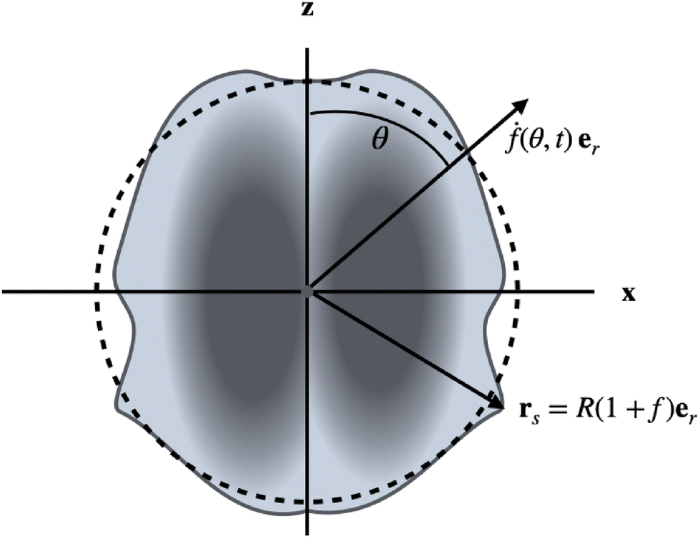
The particles are driven by small, time-dependent deformations of nearly spherical shapes. Such deformations, caused by active forces, have been calculated for vesicles36 and droplets.35 Here we take a different point of view: we consider the time-dependent deformations as given and compute the corresponding propulsion of the particle. The deviations of the shape of a particle from a reference sphere, which has the same volume as the particle, are described by a function f (see Fig. 1), which determines the positions rs of surface points via the relationship
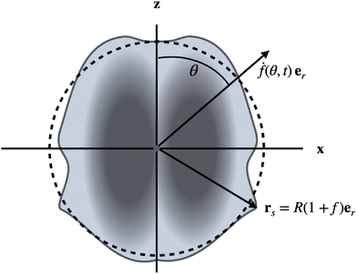 |
| | Fig. 1 Illustration of setup and notation. The (uniaxial and achiral) shape changes (drs/dt = ḟ(θ,t)er) are assumed to be radial with respect to the center of a reference sphere of radius R (dashed line), which has the same volume as the particle. The interior can be a solid or a Newtonian fluid. For a droplet, the interface is a geometric surface, whereas for a vesicle it represents an incompressible fluid membrane. | |
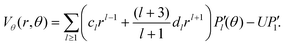
We use R as the unit of length. The driving, which we will study in this work, is given by shape changes ḟer (the dot denotes the time derivative), which are restricted to radial directions with respect to the center of the reference sphere. We therefore call this point the center of deformation in the following. The radial drive can be studied analytically for all three types of particles by using a perturbation expansion, as will be shown below. For simplicity, we also restrict our considerations to uniaxial (and achiral) deformations f(θ,t). This assumption is easily lifted, but the uniaxial case is sufficient to quantitatively compare the properties of amoeboid translational motion of the different particles. Our aim is to calculate the propulsion velocities U and the dissipated powers Ė, which result from given deformations f(t). We can expand the function f(θ,t) in Legendre polynomials
| |  | (3) |
and characterize the deformations by the amplitudes
fl. The sum does not include the term
l = 1 that would correspond to rigid body motion. For all three types of particles, the
fl are restricted by the condition that the particle volume remains constant, as the interior fluid or solid is taken to be incompressible. The time dependence of the amplitudes
fl(
t) has to be restricted to slow dynamics. More precisely we require the product of the Reynolds number and the Strouhal number to be small so that the partial time derivative in the Navier–Stokes equation can be neglected.
48
Solid bodies, vesicles, and droplets are modeled in the simplest possible way: we ignore the rheology of the interface and instead formulate appropriate boundary conditions which are presented below. The interior of vesicles and droplets consists of a Newtonian fluid with the same density as the ambient fluid, but in general with a different viscosity λη. The inner flow will contribute to the energy that is dissipated during the motion. For the solid, we do not include inner dissipation mechanisms because this would go beyond the scope of a hydrodynamical model and leaves many possibilities. As a consequence, the dissipated energy calculated from the outer flow is only a lower bound to the total dissipation of the solid particle.
All calculations will be performed in a frame, in which the center of deformation is at rest (CODF), because it is in this frame that the shapes f(θ,t) are defined. In the CODF, the flow field v(r,t) obeys the boundary condition
| |  | (4) |
at infinity. The swimming velocity
U is defined here as the velocity of the center of deformation and it points in the
z-direction, due to the uniaxial symmetry,
i.e.U =
Uez. We could have chosen any other point of a deformable particle to define its velocity. From the perspective of dynamics, the center of mass is particularly emphasized. In the CODF, it moves with a non-vanishing velocity
vcm that is easily calculated from the deformations
f(
t),
| |  | (5) |
and does not depend on the type of particle. The velocity of the center of mass
Ucm in the laboratory frame is then given by
Ucm =
U +
vcm.
The models for the particles are now completed by specifying the boundary conditions, which uniquely determine the flow field.
2.1 Deformable solid body
For a solid particle, we use no-slip boundary conditions on its surface ∂V, implying| |  | (6) |
Together with eqn (4), this determines the outer flow uniquely.
2.2 Vesicle
In the simplest model of a fluid membrane, we consider only the local inextensibility, which means that the surface divergence of the flow vanishes, that is ∇s·v(rs) = 0 for every point rs on ∂V. We can rewrite this constraint in terms of viscous tractions tvisj = niσviscij,| | | ∇s·v(r) = tvis(r)·n = 0, r ∈ ∂V. | (7) |
where n is the outward normal to the surface.
The shape evolution of the vesicle is described by a level set function H(r,θ,t) = r − rs(θ,t) = 0 for all t, which implies the kinematic equation
| |  | (8) |
The boundary condition (7) together with the kinematic eqn (8) and the far-field asymptotics eqn (4) uniquely determine the outer flow field v and the swimming velocity U for given fl and ḟl. To calculate the dissipated energy, one also needs the flow and the stress inside the vesicle, which will be denoted by V and Σ. The internal flow obeys the same boundary conditions on the membrane as the flow of the surrounding fluid.
In contrast to particles and droplets, the deformations fl of vesicles are further restricted because their surface area
| |  | (9) |
with
z = cos
![[thin space (1/6-em)]](https://www.rsc.org/images/entities/char_2009.gif) θ
θ, remains constant. Instead of
A, we will use the excess area
Δ, defined by the relation
A = 4π
R2(1 +
Δ), to express this restriction.
46
2.3 Droplet
The droplet consists of an incompressible Newtonian fluid with viscosity λη. The internal and external fluids are completely immiscible and are therefore separated by a sharp interface characterized by a constant surface tension. We use lower case symbols for the exterior and upper case symbols for the interior of the droplet. The inner flow field (which is again indicated by V) must remain finite in the center of deformation.
The boundary conditions require continuity of the flow across the interface
In the following, we also assume continuity of the tangential tractions
| | | (δij − ninj)(tj(r) − Tj(r)) = 0, r ∈ ∂V. | (11) |
This excludes inhomogeneous surface tensions or any other tangential forces at the interface and, therefore, restricts the class of possible physical mechanisms generating the deformations to active normal forces. Prominent examples of such mechanisms are droplet deformation by electric fields23,39,49,50 and deformation by polar molecules with strong anchoring.40
The balance of normal forces at the interface of a droplet with homogeneous surface tension ![[small gamma, Greek, circumflex]](https://www.rsc.org/images/entities/i_char_e0b2.gif) and normal active tractions tact = tactn is given by
and normal active tractions tact = tactn is given by
| | | n·(t(r) − T(r)) = ∇·n + tact. | (12) |
This relation is not needed to determine the flow at given f(θ,t). However, it can be used to calculate the active tractions responsible for the given deformations if desired.35 Using the expansion in small deformations, ∇·n = 2(1 − εf) − ε∇2f + ![[scr O, script letter O]](https://www.rsc.org/images/entities/char_e52e.gif) (ε2), we can write eqn (12) in linear order in ε as
(ε2), we can write eqn (12) in linear order in ε as
| | | tact = tr − Tr + (2f + ∇2f). | (13) |
This equation either determines the deformations for given active tractions or yields the active tractions for given deformations as worked out in detail in ref. 35, but is not needed here.
Just as for vesicles, the shape evolution of the droplet is described by a level set function and eqn (4), (8), (10) and (11) determine a unique solution for the outer and inner flow fields.
3 Perturbation expansion
To set up a perturbation expansion in small deformations of a spherical particle, we introduce an order counting parameter ε, which multiplies the amplitudes fl and is set to 1 at the end of the calculations. It turns out that the expansion proceeds in powers of both deformation f and its time derivative ḟ; therefore, the expansion requires f and ḟ to be of the same order of smallness. Up to the second order, the constraints of constant volume and constant surface take the form46| |  | (14) |
| |  | (15) |
The volume constraint eqn (14) will be used to eliminate f0 at (ε2).
For uniaxial and achiral systems, we expand the general external solution of Stokes equations35 in Legendre polynomials Pl(θ) and their derivatives  :
:
| |  | (16) |
| |  | (17) |
In a perturbative approach, the coefficients al and bl of the flow field are expanded in powers of ε,
| | | al = εa(1)l + ε2a(2)l + (ε3), | (18) |
| | | bl = εb(1)l + ε2b(2)l + (ε3) | (19) |
giving rise to a corresponding expansion of the flow field:
v =
εv(1) +
ε2v(2) +
(
ε3).
The perturbative analysis is carried out to the second order, since this is the minimum order that results in a non-zero swimming velocity U. In the following, we present the results for deformable solid particles, vesicles, and droplets. All three use the above expansion eqn (18) in the appropriate boundary conditions. The computations are easiest for the solid particle; we therefore give the explicit steps of the calculation for this case in the next subsection and delegate some details of the calculations for vesicle and droplet to the appendices.
3.1 Deformable solid body
As a first step we expand the boundary condition eqn (6) in powers of f,| | | v(1 + f,θ) = v(1,θ) + f∂rv(1,θ) + … = ḟer. | (20) |
To lowest order this equation reads
| |  | (21) |
with the solution
| |  | (22) |
for
l ≥ 2. The boundary condition in second order becomes
| |  | (23) |
| |  | (24) |
Substitution of the first order solution into the above equation yields
| |  | (25) |
| |  | (26) |
These equations determine the flow field as a function of the prescribed deformations to (ε2). In order to obtain the coefficients {a(2)l,b(2)l} explicitly, one has to project the above equations onto Pl,  .
.
Projection of eqn (25) onto P0 yields
| |  | (27) |
Here we have used the orthogonality of the Legendre polynomials and the constraint of constant volume,  , which guarantees that the projection onto P0 vanishes. We are mainly interested in the propulsion velocity of the particle, and hence project eqn (25) onto P1 and eqn (26) onto
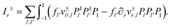
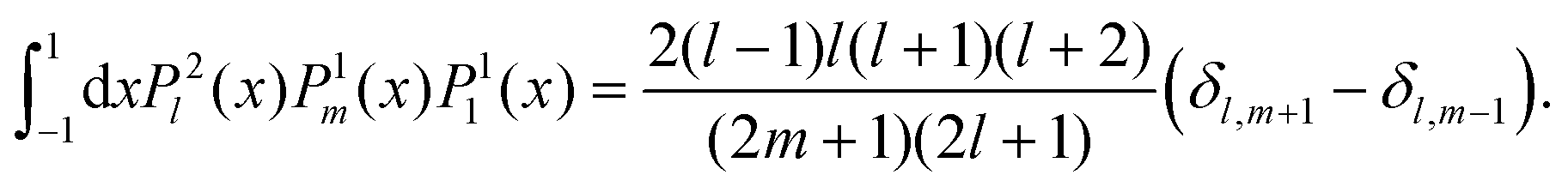
  , the latter denoting the associated Legendre polymomial P11. The calculation requires integrals of 3 associated Legendre polynomials, which are given in Appendix C. As a result of this procedure, we obtain 2 equations for a(2)1, b(2)1 and U:
| |  | (28) |
The particle has to be autonomous, that is, the total force has to vanish, which implies that the flow has to decay faster than 1/r for large r and hence b(2)1 = 0.
The solution of this system is a linear combination of the inhomogeneities (right hand sides) and therefore consists of terms proportional to flḟl+1 and to fl+1ḟl. This property also applies to the other two types of particles, so that we can always give the swimming velocity in the form
| |  | (29) |
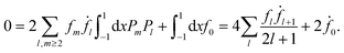
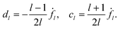
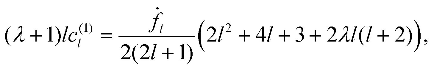
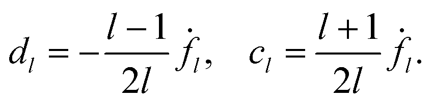
For the solid body, the coefficients Rl and Sl are obtained from eqn (28) and take on the form
| |  | (30) |
| |  | (31) |
Note that the swimming velocity of deformable solid bodies is independent of the viscosity η, and therefore, it is a purely geometric quantity.29 These results are not new, but have been derived previously, first by Lighthill25 and later corrected by Blake.26 We have presented them here in detail to demonstrate our strategy, which we now apply to both the droplet and the vesicle.
3.2 Vesicle
For the vesicle, the calculation steps are nearly identical to those used for the solid particle; it is only the form of the boundary conditions that differs. To first order, the boundary conditions (eqn (7) and (8)) read| |  | (32) |
and the solution is| |  | (33) |
To second order we get
| | | v(2)r = ḟ0 + f′v(1)θ, | (34) |
| | | σ(2)rr = 2f′σrθ(1) − f∂rσ(1)rr. | (35) |
Substituting the first-order solution from eqn (17) and (33) and the results of Appendix B, yields
| |  | (36) |
| |  | (37) |
Using both the constant volume and the constant area constraint, the projection of the above two equations onto P0 can be shown to vanish. The projections onto P1 lead to two equations for a(2)1, b(2)1 and U. We require the system to be force free, implying b(2)1 = 0, so that the resulting equations determine a(2)1 and U in second order in the deformation. The swimming velocity takes the form of eqn (29) with
| |  | (38) |
| |  | (39) |
Just as for the solid particle, the swimming velocity U does not depend on the viscosity η. The velocity U differs from the result given in ref. 36 by a total time derivative, which may arise from a different choice of reference point within the deformable vesicle.
3.3 Droplet
The analysis of the droplet requires both inner and outer solutions of the Stokes equation. The outer solutions v are taken from eqn (16) and (17), the inner solutions V are given by| |  | (40) |
| |  | (41) |
The boundary conditions in first order read
| |  | (42) |
The required stress components of the inner and outer flow are calculated in the Appendix B.
In second order the eqn (8), (10) and (11) take on the form:
| v(2)r + f∂rv(1)r − f′v(1)θ = ḟ0, |
| V(2)r + f∂rV(1)r − f′V(1)θ = ḟ0, |
| v(2)θ + f∂rv(1)θ = V(2)θ + f∂rV(1)θ, |
| | | σ(2)θr + f∂rσ(1)θr + f′(σ(1)rr − σ(1)θθ) = Σ(2)θr + f∂rΣ(1)θr + f′(Σ(1)rr − Σ(1)θθ). | (45) |
We substitute the results of the first-order solution for the velocities and stress components in the above equations, which must be solved for the coefficients a(2)1, c(2)1, ![[d with combining circumflex]](https://www.rsc.org/images/entities/i_char_0064_0302.gif) (2)1 and U. The resulting Rl and Sl in eqn (29) (and therefore also Udrop) are rational functions of the form
(2)1 and U. The resulting Rl and Sl in eqn (29) (and therefore also Udrop) are rational functions of the form
| |  | (46) |
| |  | (47) |
The second-order polynomials r(n)l(λ) and s(n)l(λ) can be found in Appendix D. Unlike a solid particle or a vesicle, the swimming velocity of a droplet depends on the viscosity contrast λ. Note that the l-components of the velocity U have well-defined limits for λ → 0 and for λ → ∞.
3.4 Center of mass velocity
The calculated swimming velocities U of the particles refer to the motion of the center of deformation in the laboratory frame. We can transform them to center-of-mass velocities in the laboratory frame by adding to U the second order result of eqn (5), given by| |  | (48) |
4 Energy dissipation
The dissipated power in an incompressible Stokes flow in a volume V is given by| |  | (49) |
Pressure does not contribute to this expression, so σij can be replaced by viscous stress σviscij. In spherical coordinates the integral takes on the form
| |  | (50) |
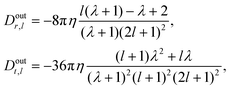
To evaluate the leading order, we need the flow field only in (ε) and the integration is over the reference sphere. For both outer and inner flow fields, the two terms are evaluated in Appendix E.
Our model does not take into account interior dissipation of the solid particle. The power due to the ambient flow,
| | 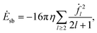 | (51) |
is therefore only a lower bound on the total dissipation.
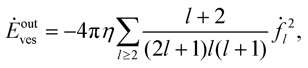
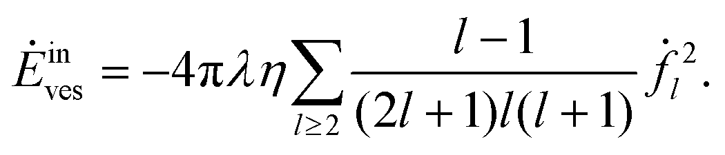
For the vesicle, the dissipated power due to the outer flow takes on the form
| | 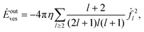 | (52) |
and the inner flow contributes
| | 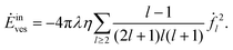 | (53) |
The l-components of outer and inner dissipation of the droplet,
| |  | (54) |
are given explicitly in Appendix E.
5 Comparisons
We will now use the general results of eqn (29) and (51)–(54) to discuss and compare the swimming velocities, the dissipation and the energetic efficiencies of the three types of particles, when they are driven by periodic deformations with period T.
As a result of Section 3, the average swimming velocities
| |  | (55) |
in second order can be represented as a sum

of terms
Ūl, which contain the time averages of
Φl(
t) =
ḟl+1fl. Note that total time derivatives, such as
vcm, do not change
Ū. Therefore, the average swimming velocity is a physical quantity that is independent of the chosen body fixed reference frame. Differences in swimming velocities between the particle types arise solely from the numerical values of
Rl −
Sl. These values are constants for the solid and the vesicle (see
Table 1), whereas for droplets they decrease with increasing viscosity contrast
λ, such that the bubble (
λ = 0) is the fastest.
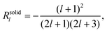
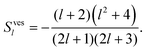
Table 1 The coefficients Rl and Sl, which determine the swimming velocities (see eqn (29)) for l = 2 and 3. These coefficients are used in Section 5.4. In the third column, μ = (λ + 1)(3λ + 2)
|
|
Solid |
Vesicle |
Droplet |
|
R
2
|
−9/35 |
−47/35 |
−3(219λ2 + 545λ + 286)/(245μ) |
|
S
2
|
−6/35 |
−32/35 |
6(−47λ2 − 61λ + 8)/(175μ) |
|
R
3
|
−16/63 |
−96/63 |
−8(23λ2 + 57λ + 31)/(63μ) |
|
S
3
|
−5/63 |
−65/63 |
(−103λ2 + 13λ + 160)/(147μ) |
In the following, we discuss two special examples in detail to illustrate our general results: (1) periodic driving with only two adjacent amplitudes flfl+1 and (2) simple harmonic motion with three adjacent amplitudes, which allow for optimization of strokes either with respect to speed or efficiency. Whenever necessary for de-dimensionalization, we use T/2π as a unit of time in the following subsections.
5.1 Swimming velocity ((l, l + 1)-strokes)
In general, the time average ![[capital Phi, Greek, macron]](https://www.rsc.org/images/entities/i_char_e0c1.gif) l depends on the detailed functional form of the deformation amplitudes fl(t) and fl+1(t). For droplets and deformable solids these amplitudes are unconstrained, but for vesicles they have to obey the area constraint eqn (15). If only one (l, l + 1)-pair of amplitudes is nonvanishing, this restricts the manifold of possible deformations to an ellipse in the (fl,fl+1)-plane, and Tl becomes the area of the ellipse,25,36 that is
l depends on the detailed functional form of the deformation amplitudes fl(t) and fl+1(t). For droplets and deformable solids these amplitudes are unconstrained, but for vesicles they have to obey the area constraint eqn (15). If only one (l, l + 1)-pair of amplitudes is nonvanishing, this restricts the manifold of possible deformations to an ellipse in the (fl,fl+1)-plane, and Tl becomes the area of the ellipse,25,36 that is| |  | (56) |
with βl = 2(2l + 1)/[(l + 2)(l − 1)]. This shows that Ū does not depend on the time course of the deformation amplitudes. For l = 2 we recover the result  given in ref. 36.
In Fig. 2, we show the speed |Ūl| of the droplet for two (l, l + 1)-pairs as a function of λ in comparison to those of a vesicle. All components Ul decrease with λ and have finite and non-vanishing limits for small and large λ as stated above. The l-dependence of the swimming speeds of a vesicle and a solid body are shown in the inset of Fig. 2.
 |
| | Fig. 2 Average swimming speed Ūl (divided by excess area Δ), generated from (fl, fl+1)-pairs, of a droplet (curved line) and a vesicle (horizontal lines) versus viscosity contrast λ for two pairs. Dotted lines correspond to l = 2, 3 and dash-dotted lines to l = 3, 4. The inset shows the λ-independent Ūl/Δ for a vesicle and a solid body versus l. | |
In general, all |Ūl| of droplets decrease with increasing λ. For small λ, the swimming speeds also decrease with increasing l, while for λ ≳ 1.3, they begin to increase with increasing l. Note also that unlike a vesicle the values of |Ūl| for a solid body increase for l = 2, 3 before they start to decrease significantly from l = 5.
5.2 Dissipation
In leading order, each deformation amplitude fl(t) contributes to the dissipated energy – even if only a single driving amplitude is present and the particle is not propelled. We make use of eqn (51)–(54) to compute the energy  that is dissipated in a period T. For our model of a deformable solid, Din = 0, so that Ēl is independent of λ. For a vesicle it is linear in the viscosity contrast λ, and for a drop it is the quotient of two second order polynomials in λ, multiplied by a factor λ. Due to the absence of internal dissipation, the total dissipated energy of the solid particle will always be the smallest for large λ. In Fig. 3 we compare Dl = Doutl + Dinl of vesicle and drop (with the same internal and external viscosities) to that of the solid particle for l = 2 and 3.
 |
| | Fig. 3 Dissipation coefficients Dlvs. viscosity contrast λ. Solid lines: drop, dashed lines: vesicle, dotted lines: solid particle. Upper lines refer to l = 2, lower lines to l = 3. | |
For all particle types, the dissipation coefficients Dl become smaller with increasing l. The dissipated energy is always lower for vesicles than for droplets. For droplets, D2 (D3) reaches the value of the solid particle at λ ≈ 2.9 (λ ≈ 3.4). For vesicles the crossover appears at larger values (λ ≈ 20 for l = 2 and 22 for l = 3).
5.3 Simple harmonic deformations with area constraint
For deformations consisting of more than two adjacent amplitudes fl, fl+1, the average speed Ū depends on the time course of the constrained swim strokes. In the following, we restrict the time dependence to simple harmonic motion, for which a more detailed discussion is possible. The deformations consist of a sum of terms fl(t)Pl(cosθ) with| | | fl(t) = Fl(eiαl+iωt + e−iαl−iωt). | (57) |
Such strokes lead to particle velocities
| |  | (58) |
when inserted in
eqn (29). Note that one of the phases
αl can be arbitrarily chosen by appropriately adjusting the origin of the time axis. The time-independent term is the mean swimming velocity
Ū. Fourier components with different frequencies
ωl for different
l-components do not contribute to the time average
Ū, so we can consider a single
ω without loss of generality. The choice of time unit 2π
T corresponds to
ω = 1 for the harmonic deformations.
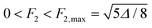
In the following, we discuss the simple non-trivial case of three l components, l = 2, 3 and 4. A swim stroke is then characterized by the parameters F2, F3, F4, α2, α3 (α4 is set to zero by choosing a suitable initial time). These five parameters must satisfy three equations, derived by inserting eqn (57) into eqn (15) and separating the time independent and time dependent parts. The resulting two-parameter manifold can be conveniently described by the l = 2 parameters F2, α2, as detailed in Appendix F. For each pair (F2, α2) there are two swim strokes, corresponding to motion in either the (+z)- or the (−z)-direction with identical speed. Consistent strokes can be found for every α2, while the range of F2 is limited to 0 ≤ F2 ≤ F2,max (in Appendix F we show that  ). Now we can compare the trajectories, the swimming velocities and the dissipated power of a solid body, a vesicle, and a drop (all three of equal volume), which execute all possible area-conserving swim strokes composed of l = 2, 3 and 4 components.
5.4 Swimming velocities with area constraint
For a comparison of average swimming velocities with constrained (l = 2, 3, 4)-swim strokes, we use the entries of Table 1. An example of trajectories for a fixed stroke is shown in Fig. 4. It illustrates that the speeds and oscillation amplitudes vary between particles, and it is even possible for the same swim stroke to propel different particles in opposite directions.
 |
| | Fig. 4 Example of trajectories: α2/2π = 0.952, F2/F2,max = 0.78, λ = 1. Solid line: droplet, dashed line:vesicle, dotted line:solid particle. The dotted straight line Ūt highlights the motion of the solid particle in the (−z)-direction. | |
The results for the average swimming velocities are summarized in Fig. 5. The parameter space of all possible constrained swim strokes lies in the (F2,α2)-plane. In the contour plots, the maxima are marked with black dots. Slices along parts of the black lines are shown in Fig. 6. The white line indicates zero propulsion velocity.
 |
| | Fig. 5 Contour plots of swimming velocity Ū over the entire parameter space (F2, α2) at λ = 1: (a) vesicle: the maximum vesicle speed (black dot) is 0.372 at F2/F2,max = 0.6224, (b) droplet: the maximum drop speed is 1.001 at F2/F2,max = 0.5081, (c) solid particle: the maximum particle speed is 0.113 at F2/F2,max = 0.4089. The slices marked by (black) solid lines are shown in Fig. 6. | |
 |
| | Fig. 6 Swimming speed along the solid lines shown in Fig. 5 near the zeros of |U|. (a) At fixed α2/2π = 0.91, (b) at fixed F2/F2,max = 0.95. | |
The general form of the dependence of Ū on the parameters F2 and α2 is the same for all three types of particles and is determined by eqn (58). The maxima of Ū are always at α2 = π and the patterns are symmetric with respect to the line α2 = π. The strokes leading to maximum swimming speed differ for the three types of particles, the F2 value being largest for vesicles and smallest for solid particles. Note that the swimming velocity reverses its direction across the white line. This line is thus a one-dimensional manifold of swim strokes, which do not propel the particle at all.
If each active swimmer is free to select the swim stroke that maximizes its velocity, the droplet wins for all λ, followed by the vesicle and the solid particle in the third position. Note that the maximum speed of the solid particle is a factor ≈10 smaller than that of the drop. However, if the three swimmers perform the same stroke, their order of ranking can change with the parameters. This can be seen in Fig. 6, which shows the swimming speed |U| versus F2/F2,max (a) and versus α2 (b) for λ = 1 along the cuts shown in Fig. 5 in the vicinity of the zeros of Ū. At each crossing of two lines in the graph, a pair of particles changes their order in the speed ranking.
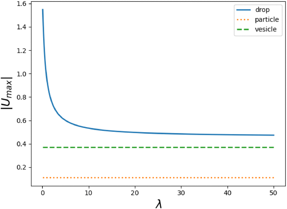
If λ is increased, the average speed of a droplet will decrease. Nevertheless, the maximum speed always remains higher than the maximum speed of the vesicle and the solid particle, as shown in Fig. 7.
 |
| | Fig. 7 Maximum speed vs. λ. The ranking (drop fastest, followed by vesicle, followed by solid particle) remains for all values of λ. | |
5.5 Lighthill efficiency with area constraint
A given swim stroke, parametrized by (F2,α2), propels different particles with different velocities, but also needs different amounts of dissipated power. A frequently used measure of the energetic efficiency of the particle is due to Lighthill.25 It is defined as the ratio of the power dissipated by a solid sphere (with the same volume as the particle) moving at the particle's mean swimming velocity Ū to the power dissipated by the particle itself, that is,| |  | (59) |
In Fig. 8, we show contour plots of the Lighthill efficiencies for a vesicle, a droplet and a solid particle at λ = 1. The lines of vanishing Ū in Fig. 5 show up here as lines of zero efficiency. In the vicinity of these zeros, the efficiencies change their order as shown in Fig. 9 for a drop and a vesicle. The efficiency of the solid particle does not vanish at the zeros of drop and vesicle but is too small to be visible on the scale of the plots. However, it is typically two orders of magnitude smaller than the efficiencies of droplets and vesicles. The small ε can already be inferred from the Fig. 3 and 5, which show that the maximum speeds of the drop and the solid particle differ by a factor of ≈10, while their dissipation coefficients Dl differ only by factors between 1 and ≈2.
 |
| | Fig. 8 Contour plots of Lighthill efficiency over the entire parameter space (F2, α2) at λ = 1 for (a) a vesicle, (b) a droplet, and (c) a solid. Dissipation from the ambient fluid and the interior (none in case of the solid) is taken into account. The maximum efficiency of a vesicle is 2.565 at F2/F2,max = 0.217, the maximum efficiency of a droplet is 3.200 at F2/F2,max = 0.364 and the maximum efficiency of a solid is 0.0280 at F2/F2,max = 0.195. | |
 |
| | Fig. 9 Lighthill efficiencies along the dashed lines of Fig. 8 near the zeros of ε. (a) At fixed α2/2π = 0.91, (b) at fixed F2/F2,max = 0.95. The insets show the full range of ε. | |
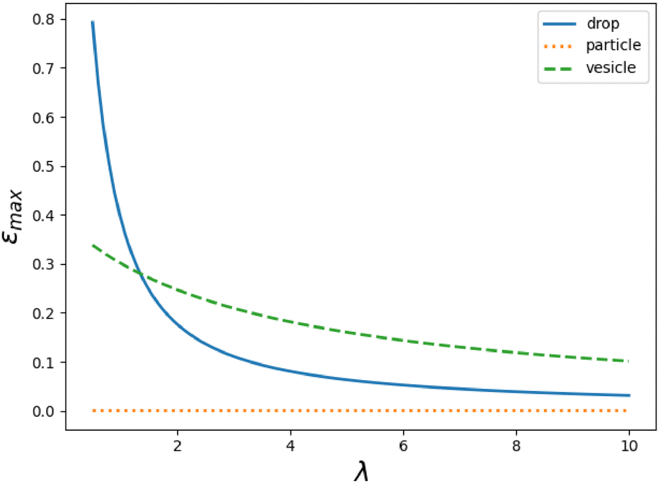
For small internal viscosities, εmax of the droplet is higher than that of the vesicle, but it decreases with increasing λ as shown in Fig. 10. When λ ≈ 1.35 the maximum efficiencies become equal, and with more viscous internal fluids the vesicle is the most efficient, although it moves slower than the droplet (as can be seen from Fig. 7). Consequently, optimizing for speed and optimizing for efficiency yield different outcomes.
 |
| | Fig. 10 Total maximum efficiency vs. λ. | |
6 Summary
In this work, we have presented a unified discussion of swimming velocities, hydrodynamic dissipation and efficiencies of three types of near-spherical amoeboid microswimmers, driven by axially symmetric achiral swim strokes consisting of radial deformations: a solid deformable body, a vesicle with incompressible fluid membrane, and a droplet. The intention of the present work is to study universal properties of this mode of swimming, which can be found in microorganisms as well as in artificial microswimmers, irrespective of the physical mechanisms generating the deformations. Our approach uses (scalar) spherical harmonics to represent surface deformations and a system of general solutions of the Stokes equation based on vector spherical harmonics. The swimming velocity and the hydrodynamic dissipation have been calculated to second order of small deformation amplitudes and their time derivatives. In our discussion, there is no need to consider the details of the physical mechanism generating the deformation if one is not interested in the additional dissipation that is caused by the mechanism. The calculated hydrodynamic dissipation is always present and represents a lower bound to the total dissipation. The restriction to axial symmetry is sufficient to compare translational motion between the three types of swimmer. The minimal models describe the types of swimmers by appropriate boundary conditions. For solids and vesicles, these conditions couple the interior material to the surrounding Newtonian fluid only via surface deformations, whereas for a droplet, the interior and the ambient flows are additionally coupled by the condition of continuity of tangential stress at the interface. As a consequence, the velocities of solids and vesicles do not depend on the viscosity ratio λ, in contrast to droplets.
To compare all three types of microswimmer, the swim strokes have to obey both the constraints of volume- and of surface-incompressibility. First, we studied swim strokes, which consist of pairs fl, fl+1 of deformations, varying periodically in time. In this case, the average swimming velocity does not depend on the detailed time course of deformations. In general, all |Ūl| of droplets resulting from fl, fl+1 decrease with increasing λ. For small λ, the swimming speeds also decrease with increasing l, while for λ ≳ 1.3, they begin to increase with increasing l. Note also that unlike a vesicle the values of |Ūl| for a solid body increase for l = 2, 3 before they start to decrease significantly from l = 5. In a next step, we have constructed a two-dimensional manifold of simple harmonic strokes, which contains l modes up to l = 4 and can be parametrized by the l = 2 parameters F2 and α2. This allows us to present the results for the swimming velocities U and the efficiencies ε in a clear and complete form as contour plots.
From these plots, the results of races between the three microswimmers are easily obtained. When each swimmer can choose the stroke that maximizes its speed, the droplet always comes first regardless of λ, although its velocity decreases as λ increases. The vesicle comes second, while the solid particle comes third. However, if the three swimmers perform the same stroke, their order of ranking can change with the parameters.
Optimizing the Lighthill efficiency and optimizing the swimming velocity result in different optimal swim strokes and rankings. The maximum total efficiency (based on the dissipation in the interior and surrounding flow) of a droplet is greater than that of a vesicle only if the dissipation ratio λ is small. Beyond λ ≈ 1.35 the maximum efficiency of the droplet falls below that of the vesicle. In all cases, the efficiency of the solid is typically two orders of magnitude smaller than that of vesicles and droplets, except in the vicinity of zeros of the efficiency. The efficiency of the solid particle will drop further if internal viscosity mechanisms are included in the model of the solid.
Experimental studies of the dependence of propulsion velocities on the time sequence of deformations require the control over particle shapes. For clean and surfactant-covered droplets, this becomes possible through the application of time-dependent electric fields.50 For a typical experiment, a glass-walled box with electrodes embedded on opposite sides is filled with the ambient liquid. A comparison with our model, which restricts the forces at the interface to radial directions, requires negligible electric currents in the ambient fluid because these would generate tangential electro-hydrodynamical tractions. Droplets are dispersed using a micro-pipette, high voltage is applied via the electrodes, and the droplet dynamics is captured by cameras. To compare our results of hydrodynamic dissipation and efficiencies with experimental results, one must be able to split the total dissipation into the internal and hydrodynamic parts or provide a driving mechanism with negligible internal dissipation. For magnetic field-driven microswimmers, the Lighthill efficiency has been directly measured.51
Our work can be extended in several directions. First, the restriction to axially symmetric swim strokes can be lifted by using deformation amplitudes f(t,θ,ϕ), which depend on both polar angle θ and azimuthal angle ϕ, and expanding f in spherical harmonics. The calculational strategies presented above can be used if the set of vector spherical harmonics is enlarged to include rotational motion.20 Furthermore, it is possible to study deformations other than radial (such as normal or tangential) by starting from appropriate variants of eqn (2). This brings our model closer to physical mechanisms like Marangoni flows or deformations by an active cytosceleton, which include tangential deformations. Second, the complete internal and ambient flow can be calculated, by projecting the boundary conditions onto higher l-components. Third, surface or body forces (for example Marangoni forces), which generate the deformations f, can be included. This makes the model more difficult because the relation between forces and deformations becomes a differential equation and introduces new relaxation time scales. For vesicles with well-separated relaxation time scales, an approach to this problem can be found in ref. 36. Finally, the internal materials of the particles may be changed to complex (for example visco-elastic) fluids or elastic solids.
Author contributions
Both authors contributed equally.
Data availability
All data is contained in the article.
Conflicts of interest
There are no conflicts to declare.
Appendices
A First-order solution for the droplet
We insert the expansions introduced in eqn (16), (17), (40) and (41) in the first-order boundary conditions eqn (42)–(44), use eqn (68) for the stress, and project on fixed l components. The resulting 4 × 4 linear system takes on the form| | | −(l + 1)(a(1)l − b(1)l) = ḟl, | (60) |
| | | l(c(1)l + d(1)l) = ḟl, | (61) |
| |  | (62) |
| |  | (63) |
The four equations are easily reduced to two, because interior and exterior of the droplet are decoupled in the first two of them, implying
| |  | (64) |
Substituting these expressions into eqn (62) yields the following equation:
| |  | (65) |
Together with eqn (63) this fixes the coefficients c(1)l and a(1)l:
| |  | (66) |
| |  | (67) |
The remaining coefficients b(1)l and d(1)l are obtained from eqn (64).
B Stress components
The first-order stress components for the exterior flow, which are used in the boundary conditions of the vesicle and the droplet are calculated from| |  | (68) |
Substituting the flow velocity from eqn (16) and (17), we find for the off-diagonal component:
| |  | (69) |
Concerning diagonal components, we only need the deviatoric stress Δσ = σrr − σθθ, which is independent of the pressure. To first order it needs to be evaluated at r = 1 and we get
| |  | (70) |
eqn (68) apply equally well to the interior flow field and yield
| |  | (71) |
| |  | (72) |
for the corresponding stress components.
C Integrals
In this appendix, we summarise the integrals over products of associated Legendre polynomials which are needed in the main text, when projecting onto P1:| |  | (73) |
| |  | (74) |
| |  | (75) |
| |  | (76) |
D Droplet 2nd order
We start from the four eqn (45), multiply the first two by P1 and the remaining 2 by P11, and integrate over z = cosθ to project onto the l = 1 mode. The resulting 4 × 4 system of linear equations takes on the formwith| |  | (81) |
| |  | (82) |
| |  | (83) |
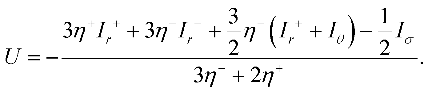
Here, v+ = v and v− = V. The term Δσ represents the deviatoric stress, defined as σrr − σθθ, while the angular brackets signify the discontinuity across the surface of the unit sphere, that is, [A(r,θ)] = A(1 − ε,θ) − A(1 + ε,θ) for ε → 0+. The velocity and the stress fields in the inhomogeneities are obtained from the first-order solutions given by eqn (64), (66) and (67) and (69)–(72). The swimming velocity U is obtained from the system (77)–(80) in the form
| |  | (84) |
To evaluate the four inhomogeneities I±r, Iθ, Iσ we insert the expansions eqn (16), (17), (40) and (41) and (69)–(72) in eqn (81)–(83) and perform the integrations with the help of eqn (73)–(76). As an example, consider I±r. It consists of a double sum of terms arising from  , from
  and from
  . It takes on the form
| |  | (85) |
We insert eqn (73) and (74) and perform the summation over l′. The remaining l-series can be written in the form
| |  | (86) |
with
| |  | (87) |
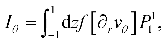
The other terms are treated in the same way. Iθ contains terms  and gives the following result:
| |  | (89) |
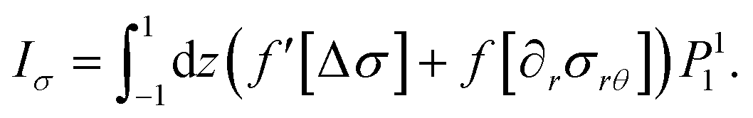
The inhomogeneity Iσ contains terms  from f∂rσθr. The contributions from f′Δσ produce terms
  (denoted by f′Δσ(0)) and terms
  (denoted by f′Δσ(2)), which can be read from eqn (70) and (72). The resulting l-series takes on the form
| |  | (90) |
All first-order quantities are proportional to ḟl, so that the result for U can be written in the form of eqn (29) in the main text.
The explicit calculation of the terms Rdropl, Sdropl and Ūl is straightforward but tedious, if not done with the help of computer algebra. The polynomials r(n)l(λ), s(n)l(λ) in eqn (46) and (47) take on the form
| |  | (91) |
and
| |  | (92) |
These expressions complete the analytical solution of the drop velocity.
E Energy dissipation
For the outer flow fields eqn (16) and (17) and the inner flow fields eqn (40) and (41), the integral eqn (50) can be evaluated by inserting the first-order solutions. For outer flow one gets| |  | (93) |
| |  | (94) |
The energy dissipation for the inner space can equally well be computed and results in
| |  | (95) |
| |  | (96) |
The flow inside the vesicle can be calculated in analogy to the outside flow and yields
| |  | (97) |
After inserting the first-order solutions into these expressions, one gets the eqn (51)–(54). For the droplet, the dissipation coefficients take on the explicit form
| |  | (98) |
and
| |  | (99) |
F Swim strokes with fixed surface area
With the designation| |  | (100) |
we find constraint equations from eqn (15) and (57), which take on the simple form| |  | (101) |
| |  | (102) |
We restrict the deformations to the three l components l = 2, 3 and 4. For F4 ≠ 0, we eliminate g4 = 1 − g2 − g3 in eqn (102) and write the remaining equations in the form
| | | 2ĝ3sinα3 = 1 − 2g2sin2α2, | (103) |
| | | 2ĝ3cosα3 = −2g2sinα2cosα2, | (104) |
with
ĝ3 =
g3sin
α3. First, we square and then add the two
eqn (103) and (104), and so we can express
ĝ3 in terms of
g2 and
α2. Then we can obtain sin
α3 and cos
α3 from
eqn (103) and (104) and finally,
g3 =
ĝ3/sin
α3. Note that the solutions of
eqn (103) and (104) remain unchanged for
α2 →
α2 + π. They can be written in the form
| |  | (105) |
| |  | (106) |
| |  | (107) |
with
C = 1 + 4(
g22 −
g2)sin
2α2. The phase
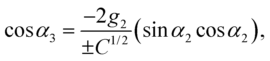
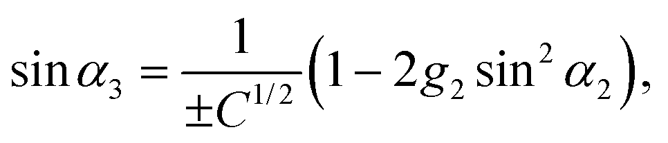
α3 is determined only up to an angle π, due to the two roots ±
C1/2. In the following, we discuss only the +-branch. Changing
α3 →
α3 + π changes the sign of the swimming velocity
U. Thus, it should always be remembered that for every motion discussed in the following, there is a corresponding motion in the opposite direction. The values of
g2 must be restricted to 0 <
g2 < 1/2 (corresponding to
) to ensure that
g3 and
g4 are positive and |cos
α3| < 1.
The special case F4 = 0 has only 3 parameters F2, F3, α2. In this case g2, g3 and α2 are completely determined to g2 = g3 = 1/2, α2 = π/2, 3π/2, and no adjustable parameters remain.
References
- E. K. Paluch, I. M. Aspalter and M. Sixt, Annu. Rev. Cell Dev. Biol., 2016, 32, 469 CrossRef CAS PubMed
 .
.
- H. G. Othmer, Wiley Interdiscip. Rev.: Comput. Mol. Sci., 2019, 9, 1 Search PubMed .
- M. Abercrombie, J. E. Heaysman and S. M. Pegrum, Exp. Cell Res., 1970, 62, 389 CrossRef CAS PubMed .
- M. Bergert, A. Erzberger, R. A. Desai, I. M. Aspalter, A. C. Oates, G. Charras, G. Salbreux and E. K. Paluch, Nat. Cell Biol., 2015, 17, 524 CrossRef CAS PubMed .
-
H. Ebata, Y. Nishigami, H. Fujiwara, S. Kidoaki and M. Ichikawa, Amoeboid movement utilizes the shape coupled bifurcation of an active droplet to boost ballistic motion, arXiv, 2024, preprint, arXiv:2402.03759 DOI:10.48550/arXiv.2402.03759.
- N. P. Barry and M. S. Bretscher, Proc. Natl. Acad. Sci. U. S. A., 2010, 107, 11376 CrossRef CAS PubMed .
- A. J. Bae and E. Bodenschatz, Proc. Natl. Acad. Sci. U. S. A., 2010, 107, E165 CAS .
- M. Arroyo, L. Heltai, D. Millan and A. DeSimone, Proc. Natl. Acad. Sci. U. S. A., 2012, 109, 17874 CrossRef CAS PubMed .
- S. Michelin, Annu. Rev. Fluid Mech., 2023, 55, 77–101 CrossRef .
- H. Boukellal, O. Campas, J.-F. Joanny, J. Prost and C. Sykes, Phys. Rev. E:Stat., Nonlinear, Soft Matter Phys., 2004, 69, 061906 CrossRef PubMed .
- E. A. Shah and K. Keren, eLife, 2014, 3, e01433 CrossRef PubMed .
- M. Weiss, J. Frohnmayer, L. Benk, B. Haller, J. J. T. Heitkamp, M. Börsch, R. Lira, R. Dimova, R. Lipowsky, E. Bodenschatz, J. Baret, T. Vidakovic-Koch, K. Sundmacher, I. Platzman and J. Spatz, Nat. Mater., 2017, 17, 89–96 CrossRef PubMed .
- S. Palagi and P. Fischer, Nat. Rev. Mater., 2018, 3, 113–124 CrossRef CAS .
- A. Mateos-Maroto, F. Ortega, R. G. Rubio, J.-F. Berret and F. Martínez-Pedrero, Particle, 2019, 36, 1900239 CAS .
- C. Abaurrea-Velasco, T. Auth and G. Gompper, New J. Phys., 2019, 21, 123024 CrossRef .
- H. R. Vutukuri, M. Hoore, C. Abaurrea-Velasco, L. van Buren, A. Dutto, T. Auth, D. A. Fedosov, G. Gompper and J. Vermant, Nature, 2020, 586, 52–56 CrossRef CAS PubMed .
-
R. Golestanian, Active Matter and Nonequilibrium Statistical Physics: Lecture Notes of the Les Houches Summer School, Oxford University Press, 2022, ch. 8, vol. 112 Search PubMed .
- A. Callen-Jones, Front. Cell Dev. Biol., 2022, 10, 1000071 CrossRef PubMed .
- R. Kree and A. Zippelius, Eur. Phys. J. E:Soft Matter Biol. Phys., 2021, 44, 6 CrossRef CAS PubMed .
- R. Kree and A. Zippelius, Eur. Phys. J. E:Soft Matter Biol. Phys., 2022, 45, 15 CrossRef CAS PubMed .
- R. Kree, L. Rückert and A. Zippelius, Phys. Rev. Fluids, 2021, 6, 034201 CrossRef .
- A. R. Sprenger, V. A. Shaik, A. M. Ardekani, M. Lisicki, A. J. T. M. Mathijssen, F. Guzmán-Lastra, A. M. M. Hartmut Löwen and A. Daddi-Moussa-Ider, Eur. Phys. J. E: Soft Matter Biol. Phys., 2020, 43, 58 CrossRef CAS PubMed .
- G. Taylor, Proc. R. Soc. London, Ser. A, 1966, 291, 159–166 Search PubMed .
- G. Taylor, Proc. R. Soc. London, Ser. A, 1951, 209, 447 Search PubMed .
- M. J. Lighthill, Commun. Pure Appl. Math., 1952, 5, 109 CrossRef .
- J. R. Blake, J. Fluid Mech., 1971, 46, 199 CrossRef .
- E. Lauga and T. Powers, Rep. Prog. Phys., 2009, 72, 096601 CrossRef .
- O. S. Pak and E. Lauga, J. Eng. Math., 2014, 88, 1–28 CrossRef .
- A. Shapere and F. Wilczek, J. Fluid Mech., 1989, 198, 557 CrossRef .
- B. U. Felderhof and R. B. Jones, Phys. A, 1994, 202, 94 CrossRef .
- B. U. Felderhof and R. B. Jones, Phys. A, 1994, 202, 119 CrossRef .
- A. Shapere and F. Wilczek, J. Fluid Mech., 1989, 198, 587 CrossRef .
- B. U. Felderhof and R. B. Jones, Phys. Rev. E:Stat., Nonlinear, Soft Matter Phys., 2014, 90, 023008 CrossRef CAS PubMed .
- Q. Wang and H. G. Othmer, J. Math. Biol., 2018, 76, 1699 CrossRef PubMed .
- R. Kree and A. Zippelius, Phys. Fluids, 2023, 35, 042002 CrossRef CAS .
- A. Farutin, S. Rafai, D. K. Dysthe, A. P. Duperrey, P. Peyla and C. Misbah, Phys. Rev. Lett., 2013, 111, 228102 CrossRef PubMed .
- M. Morozov and S. Michelin, J. Fluid Mech., 2018, 860, 711–738 CrossRef .
- N. Yoshinaga, Phys. Rev. E:Stat., Nonlinear, Soft Matter Phys., 2014, 89, 012913 CrossRef PubMed .
- S. Torza, R. Cox and S. Mason, Proc. R. Soc. London, Ser. A, 1971, 269, 295–319 Search PubMed .
- L. Giomi and A. DeSimone, Phys. Rev. Lett., 2014, 112, 147802 CrossRef PubMed .
- T. Ohta, J. Phys. Soc. Jpn., 2017, 86, 072001 CrossRef .
- E. J. Campbell and P. Bagchi, Phys. Fluids, 2017, 29, 101902 CrossRef .
- Q. Wang and H. G. Othmer, J. Math. Biol., 2016, 72, 1893 CrossRef PubMed .
- A. Moure and H. Gomez, Phys. Rev. E: Stat., Nonlinear, Soft Matter Phys., 2016, 94, 042423 CrossRef PubMed .
- G. I. Taylor, Proc. R. Soc. London, Ser. A, 1934, 146, 501–523 CAS .
- U. Seifert, Eur. Phys. J. B, 1999, 8, 405–415 CrossRef CAS .
- J. M. Rallison, J. Fluid Mech., 1980, 98, 625–633 CrossRef .
-
S. Kim and S. J. Karrila, Microhydrodynamics: Principles and Selected Applications, Dover Publ., 2005 Search PubMed .
- D. Das and D. Saintillan, J. Fluid Mech., 2017, 810, 225–253 CrossRef .
- M. S. Abbasi, H. Farooq, H. Ali, A. H. Kazim, R. Nazir, A. Shabbir, S. Cho, R. Song and J. Lee, Materials, 2020, 13, 2984 CrossRef CAS PubMed .
- C. Calero, J. García-Torres, A. Ortiz-Ambriz, F. Sagués, I. Pagonabarraga and P. Tierno, Nanoscale, 2019, 11, 18723–18729 RSC .
|
| This journal is © The Royal Society of Chemistry 2025 |
Click here to see how this site uses Cookies. View our privacy policy here. 
 Open Access Article
 This Open Access Article is licensed under a
  * and
Annette
Zippelius
*
* and
Annette
Zippelius
*


 :
:


 .
.
 , which guarantees that the projection onto P0 vanishes. We are mainly interested in the propulsion velocity of the particle, and hence project eqn (25) onto P1 and eqn (26) onto
  , the latter denoting the associated Legendre polymomial P11. The calculation requires integrals of 3 associated Legendre polynomials, which are given in Appendix C. As a result of this procedure, we obtain 2 equations for a(2)1, b(2)1 and U:


 of terms Ūl, which contain the time averages of Φl(t) = ḟl+1fl. Note that total time derivatives, such as vcm, do not change Ū. Therefore, the average swimming velocity is a physical quantity that is independent of the chosen body fixed reference frame. Differences in swimming velocities between the particle types arise solely from the numerical values of Rl − Sl. These values are constants for the solid and the vesicle (see Table 1), whereas for droplets they decrease with increasing viscosity contrast λ, such that the bubble (λ = 0) is the fastest.

 given in ref. 36.

 that is dissipated in a period T. For our model of a deformable solid, Din = 0, so that Ēl is independent of λ. For a vesicle it is linear in the viscosity contrast λ, and for a drop it is the quotient of two second order polynomials in λ, multiplied by a factor λ. Due to the absence of internal dissipation, the total dissipated energy of the solid particle will always be the smallest for large λ. In Fig. 3 we compare Dl = Doutl + Dinl of vesicle and drop (with the same internal and external viscosities) to that of the solid particle for l = 2 and 3.


 ). Now we can compare the trajectories, the swimming velocities and the dissipated power of a solid body, a vesicle, and a drop (all three of equal volume), which execute all possible area-conserving swim strokes composed of l = 2, 3 and 4 components.


 , from
  and from
  . It takes on the form


 and gives the following result:
 from f∂rσθr. The contributions from f′Δσ produce terms
 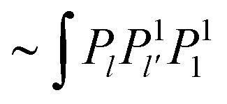 (denoted by f′Δσ(0)) and terms
  (denoted by f′Δσ(2)), which can be read from eqn (70) and (72). The resulting l-series takes on the form


 ) to ensure that g3 and g4 are positive and |cos