
 Open Access Article
 This Open Access Article is licensed under a
 Creative Commons Attribution 3.0 Unported Licence
Role of biofuels, electro-fuels, and blue fuels for shipping: environmental and economic life cycle considerations†
Fayas Malik
Kanchiralla
 *a,
Selma
Brynolf
a and
Alvar
Mjelde
b
*a,
Selma
Brynolf
a and
Alvar
Mjelde
b
aChalmers University of Technology, Department of Mechanics and Maritime Sciences, Maritime Environmental Sciences, Gothenburg, SE-412 96, Sweden. E-mail: fayas.kanchiralla@chalmers.se; Tel: +46 31 7721439
bDNV AS, Veritasveien 1, Høvik, Norway
First published on 9th August 2024
Abstract
The global shipping industry is under increasing scrutiny for its contribution to greenhouse gas emissions, and it is a challenge to find sustainable and cost-efficient solutions to meet new and stringent climate reduction targets. This study uses life cycle assessment and life cycle costing to evaluate five main decarbonization strategies to reduce climate impact from ships: uptake of e-fuels, blue-fuels, biofuels, battery electric propulsion, and onboard carbon capture technology. The environmental impact, the economic performance, and the total costs of abating carbon emissions of a total of 23 decarbonization pathways are investigated. The life cycle assessment and life cycle costing are performed on prospective scenarios considering three ship types: bulk carrier, container ship, and cruise ship, and incorporate future development uncertainties. The results show that electro-fuels in the form of e-ammonia, e-methanol, and e-liquid hydrogen in fuel cells offer the highest climate mitigation potential of more than 85% compared to the use of marine gas oil in internal combustion engines. Biofuel options have a reduction potential of up to 78%, while blue-fuel and onboard carbon capture have lower climate reduction potentials of up to 62% and 56%, respectively. Bio-methanol has the most promising cost outlook with a carbon abatement cost of around 100€ per tCO2eq. Onboard carbon capture technologies have a carbon abatement cost of around 150–190 € per tCO2eq. While they can serve as a short-term transitional solution, they have a higher environmental impact and offer limited potential for climate mitigation. E-Ammonia appears as one of the most cost-effective solutions among e-fuels. Development of policy measures and investments in renewable energy infrastructure are necessary for the growth of e-fuels production, as affordable and renewable electricity is vital for the viability of e-fuels in shipping. The uncertainty and sensitivity analysis show the influence of primary energy sources on carbon abatement costs which will be key to understand the effectiveness of policies and to develop strategies to support the shipping industry's transition to a sustainable future.
Broader contextSeveral discussions are ongoing concerning the imperative task of decarbonizing the maritime sector, with the International Maritime Organization (IMO) overseeing global deliberations while the European Union (EU) addresses some of the regional concerns. However, current knowledge gaps on a systemic level impede the ability to make informed policy decisions to find sustainable and economically feasible solutions. This study enhances system knowledge through an in-depth life cycle assessment and life cycle costing that assesses five decarbonization strategies: use of electro-fuels, blue-fuels, biofuels, battery-electric propulsion, and onboard carbon capture technologies. We analyzed environmental trade-offs and the potential of various pathways to align policy decisions toward meeting the climate targets. Additionally, the identification of key parameters, which may act as either drivers or barriers, is facilitated through uncertainty analysis and subsequent sensitivity assessments. The costs of reducing carbon emissions among different decarbonization strategies is also compared to help reveal economic trade-offs, while sensitivity analysis provides information on how the choice of primary energy sources impact the results. |
1. Introduction
Ships carry 80% of the volume of global trade1 making them crucial for international trade. Besides being responsible for nearly three percent of global anthropogenic greenhouse gas (GHG) emissions,2 emission of a wide variety of pollutants (such as sulfur oxides (SOx), nitrogen oxides (NOx), particulate matter (PM), and hydrocarbons (HC)) adversely affect air quality, leading to premature deaths3 and also have long-term effects on the natural environment and human health.4,5 In addition to energy efficiency measures, the shipping sector needs to adopt decarbonization strategies such as low climate impact energy carriers or carbon abatement technologies to achieve the net-zero GHG emissions targets for international shipping by 2050 set by the International Maritime Organization (IMO).6 Also, shipping is included in the EU “Fit for 55” package to achieve the EU's carbon neutrality. One element in “Fit for 55” is the Fuel EU Maritime regulation which aims to decrease GHG emissions by reducing the yearly average GHG intensity of energy used on board a ship from a 2020 reference value of 91.16 grams of CO2 equivalent per MJ, by 2% in 2025 and increasing by time to 80% by 2050.7 The switch towards low-climate impact energy carriers could also reduce emissions of other pollutants, resulting in additional environmental benefits.8,9Presently, most of the ships consume fossil fuels, predominantly heavy fuel oil (HFO) and marine gas oil (MGO), and the average age of the ships is increasing1 indicating more ships operating on fossil fuel will go out of service. This in combination with the projected increase in transport demand2 suggests that order bookings for new ships would likely increase in the coming years. Presently 40% of the order book can run on alternative fuels, but most are for liquefied natural gas (LNG) and only a few can run on other fuels like methanol and ammonia.1 To meet GHG emission targets, the new ships need to be able to operate on low-climate impact energy carriers.
Categories of energy carriers that are widely perceived as low-climate impact energy carriers in the shipping sector are biofuels,10–20 e-fuels,8,9,21–27 blue-fuels,15,16 and electricity from the onshore electrical grid with batteries onboard.8,9,26–28 Biofuels are fuels produced from biomass and the carbon that is released during combustion or conversion of biofuels is sequestered during biomass growth, rendering them as low-climate impact fuels.29 E-fuels or electro-fuels are synthetically produced energy carriers that contain electrolytic hydrogen (eH2) produced by the electrolysis of water using electricity, directly or chemically bonded with carbon or nitrogen.30 For carbon-based e-fuels, it is recommended that the CO2 used is captured from biogenic origin or direct air capture (DAC),30 if the carbon used is from fossil origin, the carbon emissions are only delayed.31 Blue-fuels are synthesized using the hydrogen produced by removing carbon from fossil fuels and storing the carbon permanently to prevent its release into the atmosphere and, hence limiting the life-cycle climate impact.30 The use of carbon abatement technologies onboard the ship, such as post-combustion carbon capture and storage (OCC) at exhaust when powered by fossil fuels, is another decarbonization technology.32,33 The captured CO2 can be unloaded at a port reception facility and sent to permanent storage. These previous studies were either limited to only the cost without considering the life cycle assessment or have only looked into specific types of energy carriers or technology. There is a lack of knowledge regarding the life cycle perspective of various potential low-climate impact strategies for shipping. Also, it is crucial to use consistent parameters and system boundaries when comparing the costs of carbon abatement.
The purpose of this study is to provide a comprehensive environmental and economic evaluation of five low-climate-impact strategies for selected ship types: e-fuels, blue-fuel, biofuels, battery electric, and onboard carbon capture. A total of 23 decarbonization pathways are evaluated using cradle-to-grave life cycle assessment and life cycle costing, each involving different energy carrier and propulsion system combinations. These pathways are presently at different technological readiness levels (see ESI,† Section S4) however the learning curves for this technology depend on policy support and therefore vary. The low-climate-impact strategies are compared in their future mature state, where individual technology has gone from a pilot scale to a more mature future state. In addition, two fossil-based pathways (MGO and LNG) are included as reference cases. Table 1 shows all 25 technological pathways assessed in the study and includes a combination of different fuel production pathways and different powertrain systems. Assessment is performed for three ship types with bottom-up modeling based on high-fidelity ship movement data from the automatic identification system (AIS) and ship-specific information from IHS Fairplay. Thus, this assessment allows the stakeholders to understand the balanced option that fits the selected ship type based on its ship design and operational pattern, while also considering carbon abatement costs (costs associated with reducing 1 tonne of CO2eq) for each pathway. Uncertainty and sensitivity analysis are included to understand the barriers and opportunities for the different pathways. This study is novel because it examines the environmental impacts, costs, and carbon abatement costs for five low-climate impact strategies and different energy carriers for shipping. The assessment uses consistent parameters for assessing the environmental impact and cost throughout the entire life cycle.
| Technological pathway | Shortname | Fuel production supply chain | Ship system | |
|---|---|---|---|---|
| P1 | Battery electric | BE | Wind power electricity | Battery configuration, cell type: Li-ion |
| P2 | E-ammonia in engine | eNH3ICE | Wind power electricity, electrolysis, air separation unit, and Haber Bosch. | 2S/4S ICE configuration: dual fuel |
| Pilot fuel: MGO | ||||
| P3 | E-ammonia in SOFC | eNH3FC | Wind power electricity, electrolysis, air separation unit, and Haber Bosch. | FC configuration |
| FC type: SOFC | ||||
| P4 | E-methanol in engine | eMeOHICE | Wind power electricity, electrolyzer, DAC, and Sabatier process | 2S/4S ICE configuration: dual fuel |
| Pilot fuel: MGO | ||||
| P5 | E-methanol in SOFC | eMeOHFC | Wind power electricity, electrolyzer, DAC, and Sabatier process | FC configuration; FC type: SOFC |
| P6 | E-liquid hydrogen in engine | eLH2ICE | Wind power electricity, electrolyzer, and liquefaction | 2S/4S ICE configuration: dual fuel |
| Pilot fuel: MGO | ||||
| P7 | E-liquid hydrogen in PEMFC | eLH2FC | Wind power electricity, electrolyzer, and liquefaction | FC configuration; FC type: PEMFC |
| P8 | E-liquid methane in engine | eLMGICE | Wind power electricity, electrolyzer, DAC, and Sabatier process | 2S/4S ICE configuration: dual fuel |
| Pilot fuel: MGO | ||||
| P9 | E-liquid methane in SOFC | eLMGFC | Wind power electricity, electrolyzer, DAC, and Sabatier process | FC configuration; FC type: SOFC |
| P10 | Bio-liquid hydrogen in engine | bioLH2ICE | Forest residue, biomass pretreatment, gasification, syngas cleaning, CO2 separation, and liquefaction. | 2S/4S ICE configuration: dual fuel |
| Pilot fuel: MGO | ||||
| P11 | Bio-liquid hydrogen in PEMFC | bioLH2FC | Forest residue, biomass pretreatment, gasification, syngas cleaning, CO2 separation, and liquefaction. | FC configuration |
| FC type: PEMFC | ||||
| P12 | Bio-methanol in engine | bioMeOHICE | Forest residue, biomass pretreatment, gasification, syngas cleaning, and methanol synthesis. | 2S/4S ICE configuration: dual fuel |
| Pilot fuel: MGO | ||||
| P13 | Bio-methanol in SOFC | bioMeOHFC | Forest residue, biomass pretreatment, gasification, syngas cleaning, and methanol synthesis. | FC configuration |
| FC type: SOFC | ||||
| P14 | Bio-ammonia in engine | bioNH3ICE | Forest residue, biomass pretreatment, gasification, syngas cleaning, air separation unit, and Haber Bosch. | 2S/4S ICE configuration: dual fuel |
| Pilot fuel: MGO | ||||
| P15 | Bio-ammonia in SOFC | bioNH3FC | Forest residue, biomass pretreatment, gasification, syngas cleaning, air separation unit, and Haber Bosch. | FC configuration |
| FC type: SOFC | ||||
| P16 | Bio-liquid methane in engine | bioLMGICE | Forest residue, biomass pretreatment, gasification, syngas cleaning, and methanation. | 2S/4S ICE configuration: dual fuel |
| Pilot fuel: MGO | ||||
| P17 | Bio-liquid methane in SOFC | bioLMGFC | Forest residue, biomass pretreatment, gasification, syngas cleaning, and methanation. | FC configuration |
| FC type: SOFC | ||||
| P18 | Blue-ammonia in engine | blueNH3ICE | Natural gas supply, steam methane reforming with carbon capture and storage, and Haber Bosch | 2S/4S ICE configuration: dual fuel |
| Pilot fuel: MGO | ||||
| P19 | Blue-ammonia in SOFC | blueNH3FC | Natural gas supply, steam methane reforming with carbon capture and storage, and Haber Bosch | FC configuration |
| FC type: SOFC | ||||
| P20 | Blue-liquid hydrogen in engine | blueLH2ICE | Natural gas supply, steam methane reforming with carbon capture and storage, and liquefaction | 2S/4S ICE configuration: dual fuel |
| Pilot fuel: MGO | ||||
| P21 | Blue-liquid hydrogen in PEMFC | blueLH2FC | Natural gas supply, steam methane reforming with carbon capture and storage, and liquefaction | FC configuration |
| FC type: PEMFC | ||||
| P22 | LNG in engine with OCC | LNGOCCICE | Market for LNG European mix | 2S/4S ICE w OCCS configuration: dual fuel Pilot fuel: MGO |
| P23 | MGO in engine with OCC | MGOOCCICE | Market for MGO European mix | 2S/4S ICE w OCCS configuration |
| P24 | LNG in engine | LNGICE | Market for LNG European mix | 2S/4S ICE configuration: dual fuel |
| Pilot fuel: MGO | ||||
| P25 | MGO in engine | MGOICE | Market for MGO European mix | 2S/4S configuration |
2. Methods
In this study, prospective life cycle assessment (pLCA) and life cycle costing (LCC) are conducted for three ship types based on operational data and ship-specific build data. Operational data like energy demand, fuel consumption, sailed distances, and mode of operation (maneuvering, cruising, and at sea) are derived from DNV's ‘MASTER model’ (mapping of ship tracks emissions and reduction potentials) that uses ship movement data from the AIS, detailed ship-specific information derived from ‘IHS fairplay’ and supporting data tables to estimate the energy demand, fuel consumption, and emissions of the individual ship while sailing and when in port.34,35Fig. 1 shows the framework used to estimate the life cycle environment impact and cost associated with different pathways based on the ship data. Ship-specific information is used for calculating the impact of powertrain components, storage tanks, and ship structure. The fuel consumption and operation mode are derived from the operation model of the ship. The operational model includes three main onboard energy uses: the first is the propeller load required for moving the ship, the second is the auxiliary load required for the electrical load onboard the ship required for ship operation, and the heat demand coming from the boiler which represents 2–3% of the energy use (in addition to the waste heat from the engine).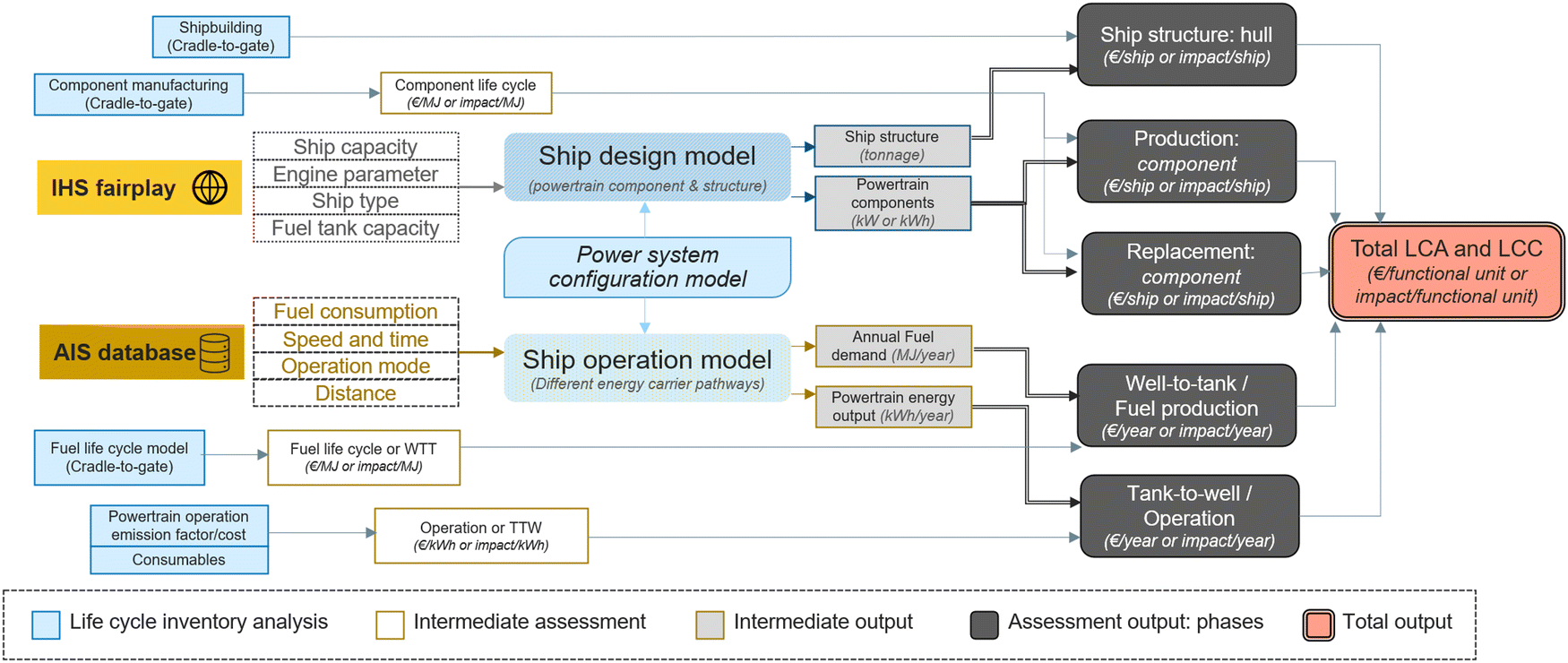 | ||
| Fig. 1 The modeling framework used in this study for assessment. | ||
2.1 Case study ships
The three ship types and ship size segments used for the study are bulk carriers (25![[thin space (1/6-em)]](https://www.rsc.org/images/entities/char_2009.gif) 000–49999 GT), container ships (50000–99999 GT), and cruise ships (≥100000 GT). These ships were selected because they specialized in different types of transport work, represent a large share of maritime goods (bulk and container) and passenger (cruise ships) transport, and were also not included in previous work by the authors. For each ship type, data reported on selected bin sizes is aggregated, and the average data of each bin size is used (Table 2). The limitation of this data is linked to uncertainties mainly related to the quality of input data, the applied model algorithms to estimate fuel consumption, and the systematics for the distribution of modeled results. The AIS model is most robust for ships when sailing. When ships are laying still, they may be performing any number of operations that cannot be modeled directly using AIS positioning data. Auxiliary and hotel loads are therefore estimated based on nominal data specific to each ship type and size. The average tank size of the current ship is oversized for the operation, and the average operation indicates that the present tank size would be capable of operating more than 50000 nautical miles. Half of the reported tank size is considered in the study, to take place which still has an operation range of more than 25000 nautical miles (in the future, oversizing of tanks is unlikely with less energy-dense fuels).
000–49999 GT), container ships (50000–99999 GT), and cruise ships (≥100000 GT). These ships were selected because they specialized in different types of transport work, represent a large share of maritime goods (bulk and container) and passenger (cruise ships) transport, and were also not included in previous work by the authors. For each ship type, data reported on selected bin sizes is aggregated, and the average data of each bin size is used (Table 2). The limitation of this data is linked to uncertainties mainly related to the quality of input data, the applied model algorithms to estimate fuel consumption, and the systematics for the distribution of modeled results. The AIS model is most robust for ships when sailing. When ships are laying still, they may be performing any number of operations that cannot be modeled directly using AIS positioning data. Auxiliary and hotel loads are therefore estimated based on nominal data specific to each ship type and size. The average tank size of the current ship is oversized for the operation, and the average operation indicates that the present tank size would be capable of operating more than 50000 nautical miles. Half of the reported tank size is considered in the study, to take place which still has an operation range of more than 25000 nautical miles (in the future, oversizing of tanks is unlikely with less energy-dense fuels).
| Ship type | Bulk carriers (25000–49999 GT) |
Container ships (50000–99999 GT) |
Cruise ships (≥100000 GT) |
|---|---|---|---|
| Number of ships | 6434 | 1049 | 103 |
| Average capacity | 65500 (DWT) |
6900 (TEU) | 4300 (pax capacity) |
| Average light displacement weight tonnage | 11165 |
27400 |
53800 |
| Average gross tonnage | 36740 |
75790 |
143550 |
| Average installed main engine (kW) | 8990 | 52650 |
67300 |
| Average installed Auxiliary engine (kW) | 390 | 2300 | 10000 |
| Average design speed (knots) | 14.2 | 24.1 | 21.1 |
| Engine type | 2-Stroke | 2-Stroke | Diesel-electric, 4-stroke |
| Service life (years) | 30 | 25 | 35 |
| Operation profile: annual energy use (GJ) | |||
| Average distance sailed per year (NM) | 84775000 |
146824000 |
144900000 |
| Average tank capacity (GJ) | 55000 |
183000 |
84000 |
| Main engine fuel use (GJ) | 159245 |
658728 |
1219189 |
| Auxiliary engine fuel use (GJ) | 22160 |
145005 |
291148 |
| Boiler fuel use (GJ) | 5 131 | 16807 |
39052 |
| Percentage time-maneuvering (%) | 5.8 | 8.4 | 6.3 |
| Percentage time-cruising (%) | 49.7 | 61.1 | 58.5 |
| Average price (million €) | 40 (min: 35; max: 45) | 125 (min: 110; max: 140) | 600 (min: 550, max: 650) |
2.2 Investigated technological pathways
The 25 technological pathways (Table 1) assessed in the study include multiple combinations of energy carriers, fuel production pathways, and different powertrain systems. Battery with electric motors is the first pathway. Internal combustion engines (ICE) and fuel cells (FC) are considered for blue-fuel pathways, biofuel pathways, and e-fuel pathways. ICE with OCC and ICE is considered for fossil fuel pathways. When ships are fueled with alternative fuels, to maintain good combustion, a pilot fuel is required27 which is assumed as fossil-MGO. Fig. 2 shows e-fuel, blue-fuel, and bio-fuel production pathways. | ||
| Fig. 2 The fuel production pathways and flows considered in the study. (a) e-Fuel production pathways, (b) biofuel production pathways, and (c) blue-fuel production pathways. | ||
The different configurations of the powertrain system included in the study are shown in Fig. 3. The selection of the size and specification of the components and energy output from the engines are calculated based on the information from the MASTER model and these power train configurations (detailed calculations are given in the ESI,† Section S1.1).
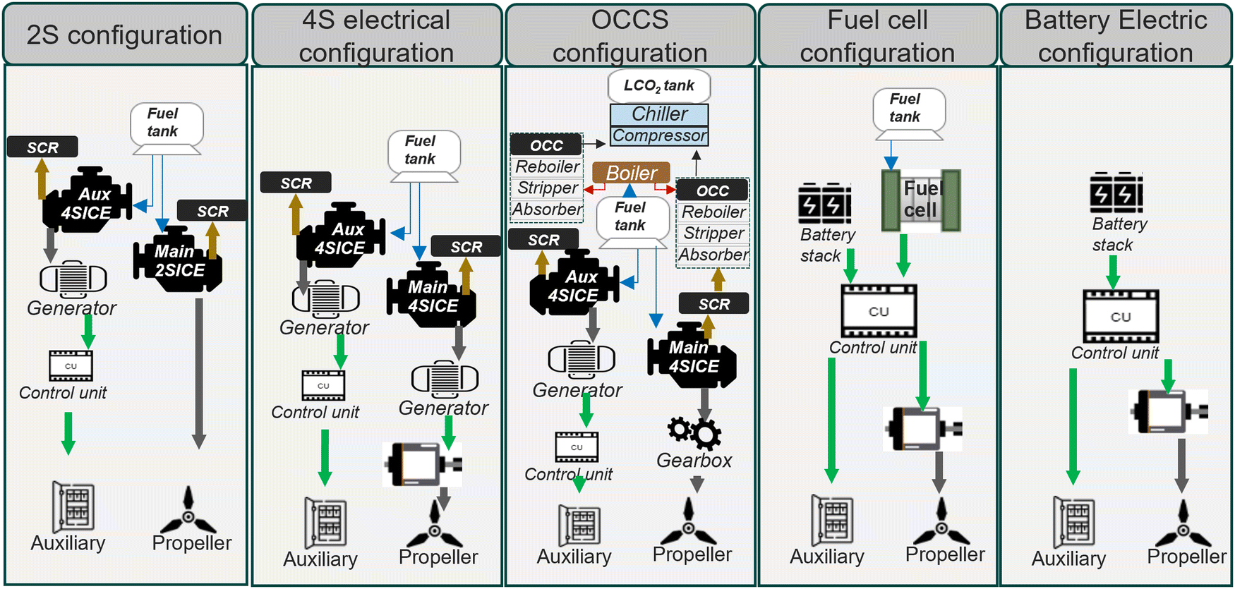 | ||
| Fig. 3 Powertrain system configurations considered in the study from tank to wake. | ||
2.3 Life cycle methodology
The ‘cradle-to-grave’ environmental impacts and cost of all pathways are calculated using the integrated life cycle framework in Kanchiralla et al.30 which is built on standard guidelines of ISO 14040 and ISO 14044.52 As recommended in the framework,30 selecting functional units, establishing system boundaries, modeling foreground and background processes, scaling up emerging technologies, and checking the robustness of results are all done uniformly and integrated with the LCC and the pLCA.| Functional unit | One DWT-NM for bulk carrier and container and one GT-NM for the cruise ship. | |
| Time horizon | When the technologies are assumed to be mature (ships built around the year 2035) | |
| Geographical boundaries | Components and ships are assumed to be produced globally. The fuel production facilities are assumed to be located 100 km from the port of operation. | |
| Cost flows | Cost in Euros (€) (with the base year 2023), considering the technical lifetime of the components and a yearly discount rate of 5%. | |
| • System boundary/life cycle phases | • Production phase (powertrain) | • Operation phase (TTW) |
| • Fuel production phase (WTT) | • Shipbuilding phase | |
| • Replacement phase (SCR/battery/FC) | ||
| • Impact categories | • Climate change, GWP100 | • Human toxicity, (cancer and non-cancer effects) |
| • Acidification | • Ecotoxicity, freshwater | |
| • Eutrophication (marine, terrestrial, and freshwater) | • Particulate matter | |
| • Resource use, (fossils, and minerals & metals) | • Photochemical ozone formation | |
| • Ozone depletion | • Ionising radiation | |
| • Land use | • Water use | |
2.3.1.1 System boundaries. Fig. 4 shows the system boundary used in the study, cradle-to-grave analysis in this study is divided into five phases: (1) fuel production phase, (2) operation phase, (3) shipbuilding phase (including end-of-life cutoff), (4) production phase (power train) (including end-of-life cutoff), (5) replacement phase (replacement of power train components) (including end-of-life cutoff). The fuel production phase or well-to-tank phase (WTT) includes processes in the supply chain of the fuel production and distribution from the extraction of primary energy and materials, production of the energy carrier, infrastructures in the fuel supply chain, and to final delivery of the fuel to the storage tanks. The operation phase or tank-to-wake (TTW) represents the processes including the use of energy carriers (e.g. combustion) onboard the ship for the propulsion and auxiliary loads. Ship building phase includes the production of ship structure and parts other than powertrain components starting from material extraction and processing. The production phase includes the production of powertrain components including energy converters and energy storage required for powering the ship and starting from the materials extraction and processing. The replacement phase includes the production of powertrain components that need to be replaced due to their relatively shorter life compared to ship life and this study includes three components: FCs, batteries, and SCR. This phase also includes materials extraction and processing for these components. The end of life of the material is analyzed using a cutoff approach, where a share of secondary raw material is assumed in the upstream input for production.
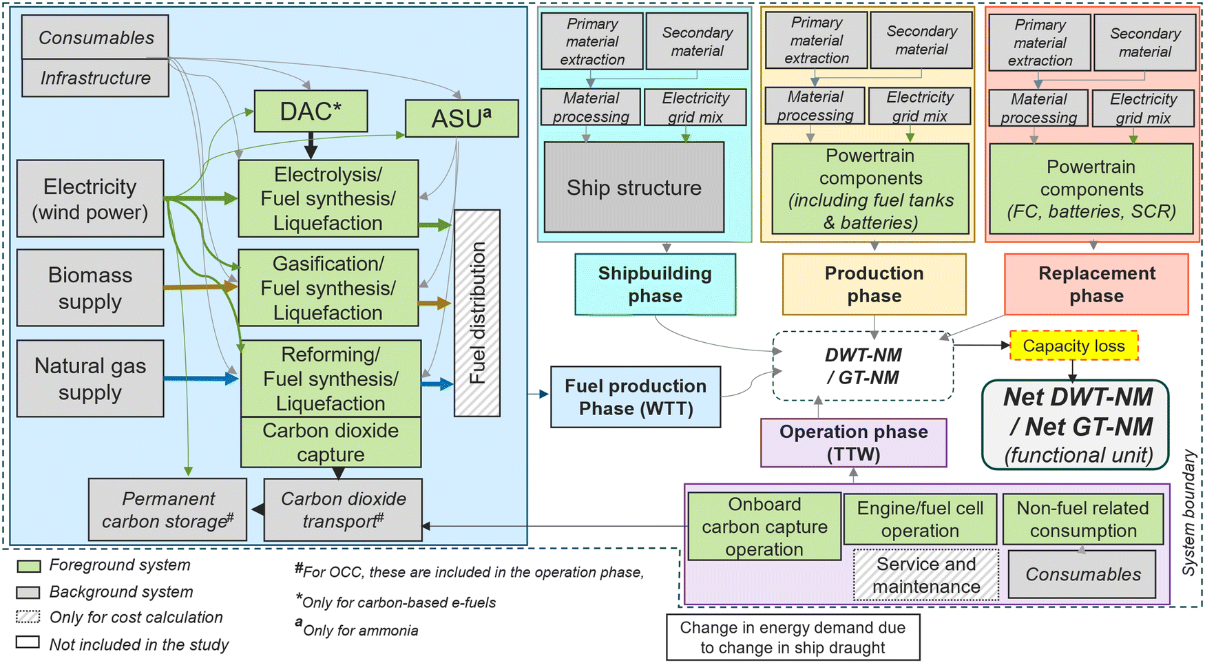 | ||
| Fig. 4 System boundary used for the pLCA and LCC assessment. Grey represents the background process and green represents foreground processes. Each phase is separated into different boxes with colored backgrounds. The boxes with patterns were not considered for LCA but for LCC assessment. | ||
For assessment, the processes within the system boundary are also divided into the foreground and background processes, as shown in Fig. 4. The foreground processes (green boxes), the focus of the study, are modeled toward a future scenario where the technology is at a mature scale.8 The input and output flows (material, energy flow, and emissions) of foreground process scenarios are developed based on literature and expert knowledge (also called expert scenarios).53 On the other hand, the background processes (gray boxes) are thought to be mature and stable, so they are not modeled in the study. Instead, they are taken straight from secondary datasets like Ecoinvent 3.8 and Gabi, or from literature. The detail on the source of data is listed in the ESI,† (Tables S4–S7).
| Operation parameter | Cost parameters | Infrastructure | |||
|---|---|---|---|---|---|
| CAPEX | O&M costa (% of CAPEX/year) | Ref. | Ref. | ||
| a Including fixed O&M cost. b Including the weight of fuel at maximum capacity, el-electricity, bio-biomass, ng-natural gas. | |||||
| Electrolysis | 50 kWhel per kgH2 | 450 € per kW | 5 | 56,57 | 56,58 |
| Haber Bosch synthesis | 0.472 kWhel per kgNH3 | 174 k€ per tNH3 per day | 5 | 37,57,59 | 60 |
| e-Methanol synthesis | 0.858 kWhel per kgMeOH | 69 k€ per tMeOH per day | 5 | 57,61,62 | 60 |
| H2 liquefaction | 6.4 kWhel per kgH2 | 2100 k€ per tLH2 per day | 4 | 63 | 63 |
| e-Methane synthesis | 0.440 kWhel per kgCH4 | 145 k€ per tCH4 per day | 5 | 38,64 | 60 |
| Methane liquefaction | 0.292 kWhel per kgCH4 | 64 k€ per tLMG per day | 5 | 65 | 60 |
| Bio-hydrogen | (2.240 kWhel + 11.79 kgbio) per kgH2 | 277 k€ per tH2 per day | 5 | 29,46 | 60,66 |
| Bio-methanol | (0.372 kWhel + 1.96 kgbio) per kgMeOH | 460 k€ per tMeOH per day | 5 | 45,47 | 60,66 |
| Bio-methane | (0.855 kWhel + 4.91 kgbio) per kgCH4 | 1157 k€ per tCH4 per day | 5 | 45,67 | 60,66 |
| Blue-hydrogen | (3.84 m3NG + (−)0.492 kWhel) per kgH2 | 250 k€ per tH2 per day | 5 | 46,49 | 49,60 |
| Blue-ammonia | (0.747 m3NG + 0.957 kWhel) per kgNH3 | 325 k€ per tNH3 per day | 5 | 48 | 48,60 |
| ASU | 0.314 kWhel per kgN2 | 376 € per kgN2 per day | 5 | 37 | 60 |
| DAC | 0.875 kWhel per kgCO2 | 271 € per kgCO2 per day | 5 | 39,68 | 39 |
| Tank, diesel | 0.02 m3 per GJ; 27.26 kg per GJb | 0.02 (€ per MJ) | 1 | 69 | 8 |
| Tank, methanol | 0.07 m3 per GJ; 57.54 kg per GJb | 0.04 (€ per MJ) | 1 | 69 | 8 |
| Tank, ammonia | 0.10 m3 per GJ; 68.64 kg per GJb | 0.08 (€ per MJ) | 1 | 69,70 | 8 |
| Tank, liquid hydrogen | 0.16 m3 per GJ; 64.21 kg per GJb | 1.67 (€ per MJ) | 1 | 70,71 | 8 |
| Tank, liquid CO2 | 1.79 kg tank per kgCO2 | 0.6 (€ per kg) | 1 | 69 | 51 |
The TTW assessment mainly depends on the emissions from ICE and FCs, as the battery-electric option is assumed an exhaust-free operation. The exhaust emission and efficiency from the ICE depend on the engine load,72 and an ICE load of 80% is assumed during cruising and 20% when maneuvering, and emission factors for different ICEs for different fuels are shown in Table 5. The variation in the specific fuel consumption for the different loads is derived using eqn (1) and based on this the fuel-related emissions are also calculated.2 The emissions and other flows are then calculated toward the total energy output from the engine which is primarily based on the propeller and auxiliary energy of the ship. This varies with the configurations depending on the efficiency of the components in the powertrain and additional load requirements for the operation of equipment (e.g. OCC).
| SFCME,load = SFCbase × (0.455 × load2 − 0.710 × load + 1.280) | (1) |
| Technology used | Dual fuel, 4S | Dual fuel, 4S | Dual fuel, 4S (Otto) | Dual fuel, 4S (LPDF) | Dual fuel, 4S (LPDF) | Dual fuel, 4S + OCC | 4S | 4S + OCC | |||||||
|---|---|---|---|---|---|---|---|---|---|---|---|---|---|---|---|
| Engine load | 80% | 20% | 80% | 20% | 80% | 20% | 80% | 20% | 80% | 20% | 80% | 80% | 20% | 80% | |
| Fuel used | Hydrogen | Ammonia | Methanol | Methane | LNG | LNG | MGO | MGO | |||||||
| a Direct use of ammonia as the reducing agent from the fuel supply. | |||||||||||||||
| Main fuel consumption (g kWh−1) | 62.0 | 64.1 | 432.3 | 447.2 | 373.6 | 386.5 | 148.7 | 153.8 | 154.9 | 160.2 | 154.9 | 183.3 | 211.9 | 183.3 | |
| Pilot fuel consumption (g kWh−1) | 9.2 | 31.8 | 9.2 | 31.8 | 9.2 | 31.8 | 9.2 | 31.8 | 9.2 | 31.8 | 9.2 | — | — | — | |
| Urea/aNH3 consumption (g kWh−1) | — | — | a 5.9 | a 5.9 | 3.3 | 3.9 | — | — | — | — | — | 8.6 | 8.6 | 8.6 | |
| Emissions (g kWh−1) | CO2 | 29 | 101 | 29 | 101 | 543 | 633 | 421 | 464 | 438 | 482 | 132 | 592 | 674 | 178 |
| CO | 0.300 | 0.700 | 0.300 | 0.700 | 1.700 | 2.200 | 3.800 | 3.800 | 3.800 | 3.800 | 3.800 | 1.000 | 1.000 | 1.000 | |
| N2O | 0.020 | 0.020 | 0.100 | 0.100 | 0.003 | 0.003 | 0.020 | 0.020 | 0.020 | 0.020 | 0.020 | 0.030 | 0.030 | 0.030 | |
| CH4 | 0.001 | 0.002 | 0.001 | 0.002 | 0.010 | 0.010 | 4.000 | 20.000 | 4.000 | 20.000 | 4.000 | 0.010 | 0.010 | 0.010 | |
| NOx | 0.700 | 0.700 | 2.600 | 2.600 | 2.600 | 2.600 | 0.700 | 0.700 | 0.700 | 0.700 | 0.700 | 2.600 | 2.600 | 2.600 | |
| NMVOC | 0.020 | 0.075 | 0.020 | 0.075 | 0.013 | 0.010 | 0.500 | 0.500 | 0.500 | 0.500 | 0.500 | 0.400 | 0.500 | 0.400 | |
| PM10 | 0.011 | 0.032 | 0.011 | 0.032 | 0.093 | 0.093 | 0.000 | 0.000 | 0.000 | 0.000 | 0.000 | 0.215 | 0.215 | 0.215 | |
| SOx | 0.018 | 0.062 | 0.018 | 0.062 | 0.018 | 0.062 | 0.018 | 0.062 | 0.018 | 0.062 | 0.018 | 0.358 | 0.414 | 0.358 | |
| NH3 | — | — | 0.050 | 0.050 | 0.025 | 0.025 | — | — | — | — | — | 0.050 | 0.050 | 0.050 | |
| CH2O | 0.0005 | 0.0005 | |||||||||||||
| Technology used | 2S | 2S | 2S | 2S | 2S | 2S + OCC | 2S | 2S + OCC | |||||||
|---|---|---|---|---|---|---|---|---|---|---|---|---|---|---|---|
| Engine load | 80% | 20% | 80% | 20% | 80% | 20% | 80% | 20% | 80% | 20% | 80% | 80% | 20% | 80% | |
| Fuel used | Hydrogen | Ammonia | Methanol | Methane | LNG | LNG | MGO | MGO | |||||||
| Main fuel consumption (g kWh−1) | 59.4 | 61.4 | 414.2 | 428.5 | 358.0 | 370.4 | 142.5 | 147.4 | 148.4 | 153.6 | 148.4 | 175.6 | 203.1 | 175.6 | |
| Pilot fuel consumption (g kWh−1) | 8.8 | 30.5 | 8.8 | 30.5 | 8.8 | 30.5 | 8.8 | 30.5 | 8.8 | 30.5 | 8.8 | — | — | — | |
| Urea/aNH3 consumption (g kWh−1) | 12.9 | 12.9 | a7.3 | a7.3 | 12.9 | 12.9 | 12.9 | 12.9 | 12.9 | 12.9 | 12.9 | 12.9 | 12.9 | 12.9 | |
| Emissions (g kWh−1) | CO2 | 37 | 106 | 28 | 97 | 529 | 615 | 426 | 500 | 444 | 517 | 89 | 571 | 659 | 110 |
| CO | 0.300 | 0.700 | 0.300 | 0.700 | 0.300 | 0.700 | 1.040 | 1.040 | 1.040 | 1.040 | 1.040 | 0.700 | 0.700 | 0.700 | |
| N2O | 0.020 | 0.020 | 0.100 | 0.100 | 0.003 | 0.003 | 0.030 | 0.030 | 0.030 | 0.030 | 0.030 | 0.030 | 0.030 | 0.030 | |
| CH4 | 0.001 | 0.002 | 0.001 | 0.002 | 0.010 | 0.010 | 0.200 | 4.000 | 0.200 | 4.000 | 0.200 | 0.010 | 0.010 | 0.010 | |
| NOx | 3.400 | 3.400 | 3.400 | 3.400 | 3.400 | 3.400 | 3.400 | 3.400 | 3.400 | 3.400 | 3.400 | 3.400 | 3.400 | 3.400 | |
| NMVOC | 0.015 | 0.060 | 0.015 | 0.060 | 0.013 | 0.010 | 0.500 | 0.500 | 0.500 | 0.500 | 0.500 | 0.300 | 0.400 | 0.300 | |
| PM10 | 0.010 | 0.030 | 0.010 | 0.030 | 0.093 | 0.093 | 0.020 | 0.020 | 0.020 | 0.020 | 0.020 | 0.215 | 0.215 | 0.215 | |
| SOx | 0.016 | 0.060 | 0.016 | 0.060 | 0.017 | 0.060 | 0.017 | 0.060 | 0.017 | 0.060 | 0.017 | 0.343 | 0.397 | 0.343 | |
| NH3 | 0.050 | 0.050 | 0.050 | 0.050 | 0.050 | 0.050 | 0.050 | 0.050 | 0.050 | 0.050 | 0.050 | 0.050 | 0.050 | 0.050 | |
| CH2O | — | — | — | — | 0.0005 | 0.0005 | — | — | — | — | — | — | — | — | |
The inventory data pertaining to the production and end-of-life stages of the components are specified in Table 6. As FC stacks, batteries, and SCR are deemed to degrade at a faster rate than other components, replacement is required according to their respective usage durations. The number of replacements is determined by comparing the life cycles of components and ships (Nrepl,i). In this study, the degradation of FCs is approximated at 0.4 percent per 1000 hours of operation, with the FC being deemed replaceable at the point of capacity loss of 20 percent.9 For battery replacement, a simplified assumption of ten years with a 60% depth of charge (DOC) as numerous factors influencing battery life (e.g., usage duration, charging cycles, and battery charging technology) are unknown and will only become apparent during the detailed design phase. Assumed inventory data for the components' raw materials is taken from the Ecoinvent 3.8 database. For ship structure, the inventory details are estimated based on the lightweight tonnage (LDT) and adopted from Jain et al.73 and raw materials data is used from the Ecoinvent 3.8 database.
| Component | Major parameter | Specific CAPEX cost | O&M cost (% of CAPEX/year) | Ref. | Material data |
|---|---|---|---|---|---|
| a Based on expert interviews. b 2% lesser efficiency is considered for NH3 ICEs due to high heat of vaporization (Table 5). | |||||
| 4SICE, diesel | 46% efficiencyme | 240 € per kW | 2 | 69 | 74,75 |
| 4SICEb, dual fuel | 46% efficiencyme | 265 € per kW | 2 | 8 | 74,75 |
| 2SICE, diesel | 48% efficiencyme | 240 € per kW | 2 | 8 | 74,75 |
| 2SICEb, dual fuel | 48% efficiencyme | 265 € per kW | 2 | 8 | 74,75 |
| PEMFC | 55% efficiencyel | 1100 € per kW | 0.5 | 76 | 77 |
| SOFC | 58% efficiencyel | 2500 € per kW | 0.2 | 8 | 78 |
| SOFC (methane) | 60% efficiencyel | 2500 € per kW | 0.2 | 8 | 78 |
| Electric motor | 95% efficiency | 120 € per kW | 1 | 79,80 | 60 |
| Gearbox | 98% efficiency | 85 € per kW | 1 | 69,79 | 75 |
| CO2 chiller | 0.0645 kWhel per kgCO2 | 102 € per kgCO2 per h | 3 | 81,82 | 60 |
| OCC | 0.027 kWhel per kgCO2 | 2000 € per kgCO2 per h | 3 | 83,84 | 85 |
| 0.85 kWhth per kgCO2 | |||||
| Alternator | 95% efficiency | 120 € per kW | 1 | 80,86 | 87 |
| SCR system | — | 40 € per kW | 2 | 88,89 | 90 |
| Battery | 70% DOD | 200 € per kWh | — | 91,92 | 93,94 |
 | (2) |
 | (3) |
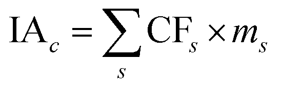
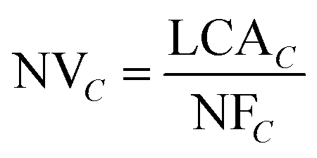
2.3.3.1 Normalization. Although as per ISO 14044 normalization is optional,52 normalization helps for better interpretation of environmental impact by providing a reference situation for the environmental pressures.97 In this analysis, the global normalization factors (NFs) from EF 3.0 with reference to the total environmental impacts.98 Normalized value (NV) is calculated using eqn (4), where c represents the impact category.
 | (4) |
 | (5) |
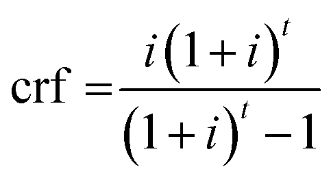
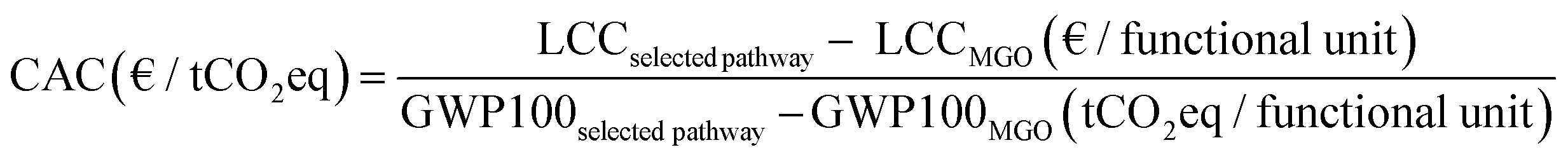
2.3.3.2 Cost assessment. Instead of focusing on material and energy flows as in LCA, LCC considers the cost flows between processes throughout the product's life cycle. The perspective of the ship's owners is emphasized in this study. Like LCA assessments, the parameters are divided into five phases. However, the ship structure, the acquisition of the propulsion system components, and the replacement of the components during replacement are related to capital investment. Hence, for cost comparison, these costs are converted to the net present value (NPV) where the future cost is discounted using the capital recovery factor (crf) given in eqn (6) and i is the discounting rate (5%). Similar to LCA, the production cost is the sum of the cost of each powertrain system component (ME, € for total powertrain system), and replacement cost is the sum of the cost of components that need to be replaced (RE, € per set of components that need to be replaced), shipbuilding is the cost of the ship excluding the powertrain system (SB, € per ship). For details on how these individual costs are calculated from inventories in Section 2.2.3, please refer to ESI,† Section S1.2 and Table S4.
 | (6) |
 | (7) |
 | (8) |
2.4 Uncertainty, sensitivity and scenario analysis
As the evaluated technologies are immature, performance parameters may undergo different changes as they mature. We conducted an uncertainty analysis based on Monte Carlo simulations to determine the impact of changing the parameters on the results, in comparison to the assumed ones. This assessment is done for both environmental and economic assessment. ESI,† Section S4 and Tables S4–S7 present the ranges of alternatives assessed in the analysis. A uniform distribution of the range of parameters was applied to the simulations 100000 times to conduct the uncertainty analysis for both the cost flows and life cycle inventory. The uncertainty analysis is done for the calculation of GWP, total cost, and CAC and it shows the ranges of environmental and cost results due to uncertainties in the development pathways for these technologies.
In addition, the results are sensitive to the cost of the primary energy carrier (which refers to electricity, biomass, and natural gas) and fuel production processes. For a better understanding of their dependencies on different decarbonization pathways, a sensitivity assessment is performed. In the cost-sensitivity assessment, the cost of the primary energy carrier was considered the most important parameter. The fuel cost and carbon abatement cost sensitivity are assessed by varying the electricity price (from 0 to 120 € per MWh), natural gas price (0–16 € per MJ), and biomass price (0–40 € per MWh). To understand the sensitivity of GWP in WTT in the CAC, sensitivity is measured by varying the carbon intensity of the electricity mix (0–150 gCO2eq per kWh), biomass gasification efficiency (30–90%), and methane leakage in the natural gas supply chain (0.5–3.5%).
In addition to the uncertainty and sensitivity analysis, a scenario analysis is performed to evaluate the impact of fuel production if an electricity mix is used instead of wind power. The following prospective LCI databases represent development in three scenarios that combine Shared Socioeconomic Pathways (SSPs) and climate targets (see ESI,† S1.5) based on their consistency in global mean surface temperature rise by 2100: SSP2-NDC (∼2.5 °C warming by 2100), SSP2-PkBudg1150 (1.6–1.8 °C warming by 2100), and SSP2-PkBudg500 (1.2–1.4 °C warming by 2100).101 The prospective LCI background databases for EU from open-source Python library premise v1.5.8102 were used for the analysis and a combination of the Ecoinvent v3.8 (system model ‘‘Allocation, cut-off by classification’’) database60 and the REMIND model103 for deriving the background process inputs.
3. Results
3.1 Environmental impact assessment
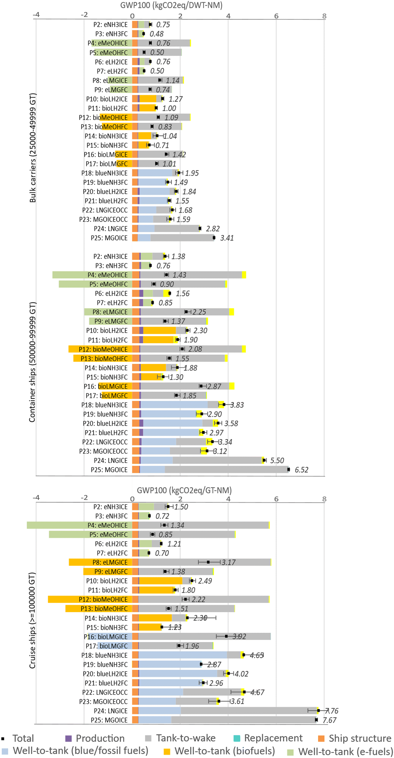 | ||
| Fig. 5 Cradle-to-grave LCA results on GWP100 per DWT-NM (bulk carrier and container ship) and GT-NM (cruise ship) for the 25 technological pathways assessed. The results are further separated into life cycle phases: well-to-tank (WTT), tank-to-wake (TTW), production of power train components, replacement of power train components, and ship structure. The upper range of the uncertainty bar from the Monte Carlo simulation represents the 90 percentile and the lower bound represents the 10 percentile. | ||
Fig. 5 shows that ship types do not significantly change the GWP reduction of the technological pathways however, there is some variation between the cruise ship and the other two ship types. This variation is mainly associated with the choice of 4S diesel-electric engines and the relatively smaller tank size for the cruise ship. A major proportion of the GWP result is attributable to WTT for all technology pathways except those based on fossil fuels (both with and without OCC). OCC options have limited potential to reduce climate impact, and a major share comes from the TTW. The TTW emissions are associated with the additional fuel burned to produce energy for the operation of carbon capture, as well as the liquefaction of the captured CO2. In addition, only a portion of the CO2 emissions are captured, and other GHGs like methane are not captured from the exhaust. The additional energy needed for the OCC system is lower for LNGICEOCC compared to MGOICEOCC; that is, a higher energy penalty and fuel are required for MGOICEOCC. However, LNGICEOCC has a lower climate reduction potential than MGOICEOCC, especially for the 4S engine type (cruise ship), because it does not capture the methane in the flue gas.
When comparing the GWP of fuel cells and engines for the same fuel, it can be noted that fuel cells have a lower GWP compared to engines. This is because fuel cells are more efficient, offer cleaner electrochemical combustion, and do not require pilot fuel, resulting in lower TTW GWP. Fuel cells have a higher impact from the manufacturing and replacement phases as more material is required for their production, but this does not outweigh the benefits. Additionally, using methane or ammonia as fuel in an engine results in a notably higher GWP compared to other alternative fuel cell options. For methane, methane slip is an issue for engines, while in fuel cells, methane slip is considered negligible due to the circulation of anode gas. Ammonia in engines has a high GWP because it can potentially produce nitrous oxide during combustion, a factor that is considered insignificant during electrochemical combustion in fuel cells.
To better understand the WTT emissions that significantly contribute to the GWP of technological systems involving e-fuels, biofuels, and blue-fuels, Fig. 6 breaks down the contributing processes into distinct categories. The lowest GWP is for liquid e-hydrogen, followed by other e-fuels. The production of liquid e-hydrogen is less complex and more efficient compared to other e-fuels, e.g., e-methanol and e-methane. As shown in Fig. 6, the energy demand is high for e-fuels, making electricity a major part of GWP for all e-fuels. This indicates that the choice of low-carbon intensity electricity is the most important aspect for e-fuels. In this study, wind power with a carbon intensity of 9 g kWh−1 is considered.104 The increased GWP for liquid e-methane, as shown in the figure, is a result of the leakage of methane during transportation and liquefaction (this also applies to bio-methane). Blue-fuels have a high GWP compared to the other fuels mainly caused by fugitive methane emissions in the natural gas supply chain (assuming 1% in the base case) and GHGs not captured in the flue gas during thermal reforming. In contrast, blue-fuels have the lowest primary energy requirement due to higher process efficiency also after considering the additional energy required for carbon capture.
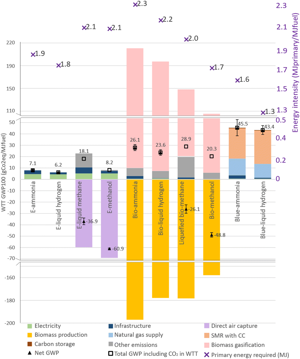 | ||
| Fig. 6 Contribution of different processes within fuel production for selected alternative fuels on climate change. | ||
Biofuels have GWP in between e-fuels and blue-fuels, and it can be seen from Fig. 6 that biomass production and gasification are crucial processes. Biomass from sustainably managed forests results in net negative emissions due to biogenic carbon uptake by trees. The low H/C ratio of wood and low gasification efficiency lead to a higher amount of biomass needed to produce 1 MJ of biofuel compared to blue-fuel production. This leads to significant CO2 removal from the atmosphere but also causes high direct biogenic CO2 emissions during gasification, as shown in Fig. 6. The net GWP for biofuel depends on GHG emissions related to forestry, transportation, energy use for chipping and drying, and process efficiencies involved in fuel production. Another observation from the result is negative GWP for carbon-containing fuel (methanol and methane) for certain stages, this is because carbon from the air is embodied in the fuel (for e-fuel, CO2 captured by DAC and for biofuel, CO2 intake during biomass growth); however, these are emitted back to the air during the fuel combustion, indicating a higher TTW GWP (also shown in figure as black squares). Liquefied bio-methane and bio-methanol have more energy-efficient production routes compared to their respective e-fuels (which require energy-intensive DAC), compared to bio-ammonia (which needs additional energy for ASU and separating CO2 from syngas) and compared to bio-liquid hydrogen (which needs energy for separating CO2 from syngas and liquefaction).
Fig. 5 also shows the capacity loss associated with a reduction in the space availability for cargo or passengers caused by different energy carriers' volumetric and gravimetric energy densities. It can be noted that container ships experience the highest cargo loss, primarily attributed to their higher fuel consumption and longer routes. Among fuel options, ammonia and liquid hydrogen have a lower volumetric energy density compared to other fuels, resulting in a higher loss of cargo capacity. Additionally, there is a significant loss of cargo capacity for the OCC options. Fuel cells, particularly SOFCs, have lower energy density compared to engines. However, they offer the advantage of lower capacity loss for the same fuel. The reason behind this is the increased efficiency of fuel cells results in a reduced need for fuel storage. The calculation of capacity loss is based on the current fuel tank capacity, which is done in a conservative manner. It is important to note that the current tanks are not designed for the longest operation needs, but they are significantly larger than necessary.
To summarize the total GWP results, e-fuels in fuel cells have the lowest climate impact, with a reduction potential of more than 85% to 91% for e-methanol, liquid e-hydrogen, and e-ammonia compared to MGO. Blue-fuels in ICE have the lowest reduction in GWP of less than 50%, and OCC has the lowest reduction potential of around 50%. Blue-fuels in fuel cells offer a reduction in GWP of around 60% compared to MGO. Biofuel in fuel cells offers a climate impact reduction potential of 70% to 80%. However, biofuels in ICE offer a climate reduction potential of around 60% to 70%. E-methane and bio-methane fueled in ICE have the lowest climate impact reduction potential compared to other e-fuel and biofuel pathways, respectively. This is due to methane slip in the engine and leakage in the distribution.
Fig. 6 and 5 display the Monte Carlo simulation results as uncertainty bars. Fig. 5 shows that the highest uncertainty is associated with ammonia in ICE (originating mainly from nitrous oxide emissions), methane in ICE (originating mainly from methane leakage), and OCC cases (originating mainly from the carbon capture rate). As technologies are under development, uncertainties around these parameters are still high. In Fig. 6, the wide range of GWP values for biofuels is mainly due to the variability introduced by gasification efficiency (±5%), while for blue-fuels, it is caused mainly by the variation added to fugitive emissions in the natural gas supply chain (±0.5%).
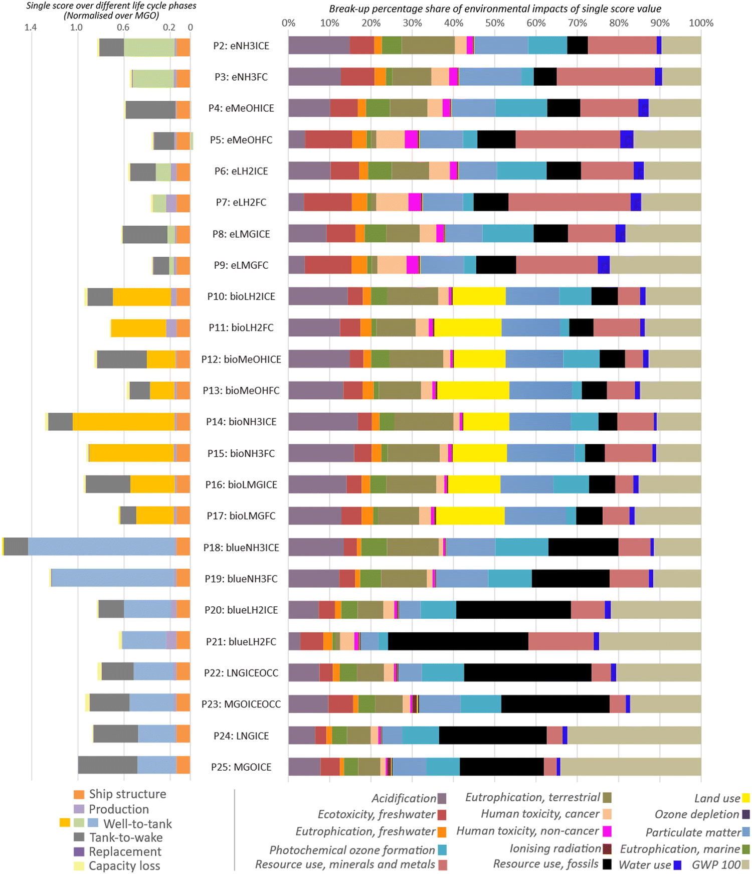 | ||
| Fig. 7 Single scored weighted average cradle-to-grave LCA results for the bulk carrier (25000–49999) for the 24 technological pathways assessed. In the left side the results are separated into life cycle phases: well-to-tank (WTT), tank-to-wake (TTW), production of powertrain components, replacement of power train components, ship structure showing the contribution of each phase to the total score and right side shows the contribution of individual impact category. | ||
The major impact categories associated with biofuels are acidification potential, land use, and eutrophication (terrestrial and freshwater) mainly associated with biomass growth and processing, as well as particulate matter associated with emissions from gasification. In the analysis, biomass from sustainable forest management (from the Ecoinvent dataset) is considered and a different source of the forest residue could change the results not only for GWP but also for all the impact categories. The quality of biomass also will affect the efficiency of the gasification process. This is particularly important as currently, the availability of sustainable biomass resources is limited, and environmental performance largely depends on the biomass source.105,106
Blue-ammonia in ICE has the highest aggregated score, surpassing the reference case. Blue-ammonia in FC is also above the reference case, while blue-hydrogen has a lower aggregated score. The major impact for these fuels is from the WTT and is related to resource use (fossils) and photochemical oxidation, which can be related to a higher amount of energy from fossil sources compared to MGO (energy loss during the natural gas reforming and additional energy required for carbon capture). OCC technological pathways have a lower overall environmental impact single score than MGO; however, this is solely due to a reduction in GWP. In all other environmental aspects, OCC options have higher impacts than MGO. The higher impact on all categories is due to the additional fuel that needs to be burned to meet the additional energy required (the engine must generate more energy) to operate the carbon capture system onboard. This leads to increased WTT (more fuel for delivering the same unit of energy to the propeller shaft) and results in more emissions of other pollutants.
Another observation that can be noted in Fig. 7 is that the fuel cells have a lower single score even after the higher impact on resource use (minerals and materials). The lower single score for fuel cells compared to engines for the same fuel can be attributed to cleaner fuel combustion, higher efficiency, and the absence of a need for pilot fuel. Ammonia has a higher impact on overall fuel pathways primarily linked to eutrophication and acidification linked to ammonia leakage in the supply chain and emission of nitrogen oxides and nitrous oxide (stronger GHG than CO2 and CH4) from engines.
3.2 Economic assessment
The LCC and CAC of the 24 different technological pathways (excluding battery-electric) for each ship type are displayed in Fig. 8. The results in the figure are ranked from the lowest to the highest CAC, indicating the most preferred option for each ship type if abatement cost is considered for decision-making. The box plot captures the uncertainty of the CAC from the Monte-Carlo simulation. The ship type is not shown to have a significant impact on the ranking of the preferred fuels; however, the CAC varies depending on the ship type. For all ship types, bio-methanol ICE appears to be the most cost-effective choice for decarbonization, with the lowest CAC (€110–150 per tCO2eq) and a low life cycle cost. Following that, OCC technologies (both using LNG and MGO) have a lower CAC between €150 and €190 per tCO2eq without considering the capacity loss. When considering the capacity loss, the CAC can reach up to 350 € per tCO2eq, as the components and additional CO2 tanks significantly reduce the capacity. Also, as shown in Section 3.1.1 the GWP reduction that can be achieved with these pathways is low. Liquid hydrogen pathways are the most cost-intensive choice for container and bulk carriers, and the cost is mainly associated with the tanks and the complex hydrogen bunkering infrastructure required in ports. The higher investment cost of tanks is due to their larger tank capacity owing to the lower volumetric energy density of liquid hydrogen compared to other energy carriers. For these ship types, which typically travel longer routes, larger tanks are needed. Although, the cruise ship cases have relatively smaller tank capacities (compared to the other case study ships), liquid hydrogen is still one of the most expensive technology choices due to its higher bunkering cost.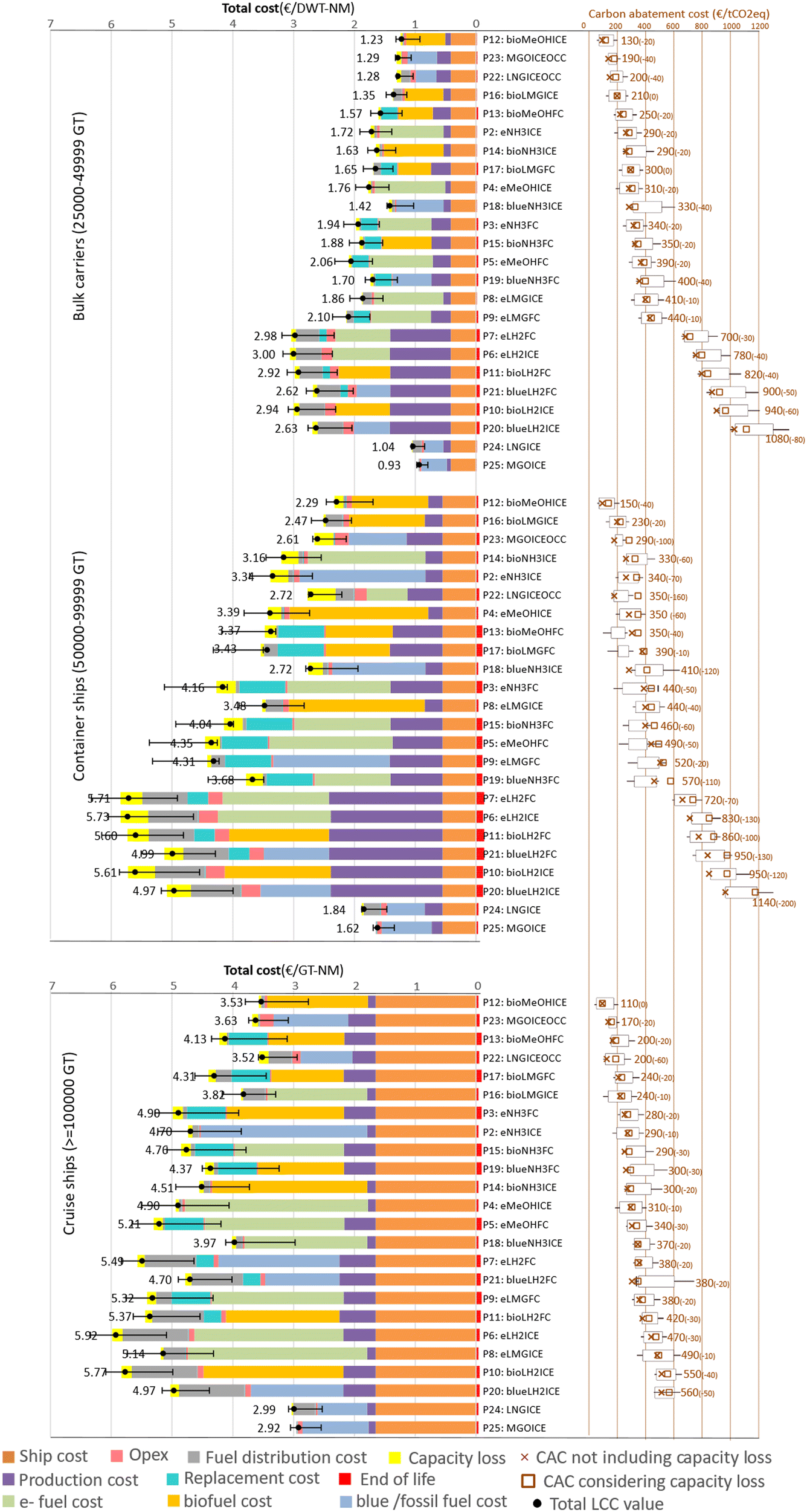 | ||
| Fig. 8 LCC results per DWT-NM (bulk carrier and container ship) and GT-NM (cruise ship) for 24 technological pathways assessed. The costs are structured separating fuel production, fuel distribution, production, replacement, and Opex. The upper range of uncertainty bar from Monte Carlo simulation represent 90 percentile and lower bound represent 10 percentile. The carbon abatement cost (CAC) is calculated for the base case considering the capacity loss and the value in the brackets shows the difference between CAC without and with capacity loss. | ||
Apart from bio-methanol and OCC options, liquefied bio-methane ICE is one of the most promising decarbonization solutions, with lower total costs and a CAC of €210–240 per tCO2eq. Even though bio-methane and bio-methanol are promising choices, e-methane, and liquefied-e-methane options have a relatively higher CAC of more than €300 per tCO2eq. The higher cost of e-methanol and e-methane is associated with the assumption that CO2 comes from an energy-intensive DAC process, whereas bio-methanol and bio-methane do not need a sub-system to source CO2 (uses biogenic carbon). Among e-fuels and blue-fuels, ammonia-based pathways have a CAC of less than €300 per tCO2eq, bio-ammonia-based pathways have a higher overall cost and CAC. Although e-ammonia fuel is more expensive than bio-ammonia and blue-ammonia, its lower GWP leads to a lower CAC. Blue-ammonia options are less expensive than other fuel options but have a high GWP, leading to a higher CAC compared to e-ammonia.
Fig. 8 demonstrates that for the same fuel, the overall cost is greater for FC alternatives than for ICE options. This suggests that the savings in fuel costs due to reduced fuel use in fuel cells are not enough to offset the higher initial investment and replacement costs of fuel cells. However, the CAC varies with ship types; this can be observed in the case of liquid methane, ammonia, and liquid hydrogen options for the cruise ship, where fuel cell options have a lower CAC than ICE options for the same fuel. This variation is associated with the investment cost of the propulsion system. The investment cost increases linearly with the installed power and utilization rate of the power system. In addition, FC needs replacement investments associated with fuel cell life compared to ship life.
Capacity loss is another important parameter that affects the CAC, a reduction in the space availability for cargo or passengers leads to loss of revenue as the operator has the same expenditure for the reduced cargo or passenger capacity. Similar to GWP change as noted in Section 3.1.1, container ships experience a notable difference in CAC due to capacity change with a difference of more than 100 € per tCO2eq for nine pathways mostly blue pathways and most importantly OCC. For cruise ships, the difference is less mainly as there are no significant changes in the gross tonnage capacity. The actual function varies with the transport mission, and the optimal design of tanks based on the range of the ship would significantly change this result. Therefore, the CAC based on the capacity loss presented is conservative.
Monte Carlo simulations show a large variation in the results compared to the base case. The large variation in the LCC and CAC is mainly linked to the uncertainties associated with fuel costs. An analysis of the cost breakdown for fuel production is shown in Fig. 9. Fuel costs are primarily determined by the price of the main energy source, i.e., biomass costs for biofuels, natural gas prices for blue-fuels, and electricity prices for e-fuels. Bio-methanol and bio-methane have the lowest cost considering other viable alternatives, owing to the lower cost of biomass and the elimination of the need for a carbon capture system. The blue-fuel pathway is comparatively less expensive for producing hydrogen and ammonia, as steam methane reforming is more energy-efficient than biomass gasification and electrolysis. Like the carbon intensity of the electricity mix, the electricity cost is critical for the e-fuel cost. Since fuel costs make up a large portion of the LCC, the cost of primary energy, which is electricity, biomass, and natural gas, also affects the LCC and CAC. Due to the limited availability of sustainable biomass, competition from other sectors could significantly impact biomass prices.
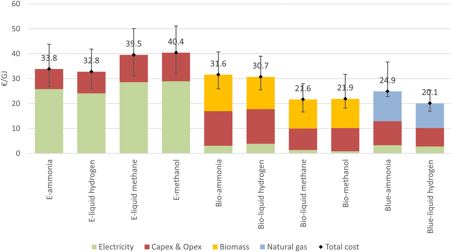 | ||
| Fig. 9 Break down of the fuel cost based on the cost of electricity, investment and operation (capex & opex), biomass, and natural gas. The ranges represent the 10 and 90 percentile from the Monte Carlo simulation. | ||
Fig. 10a displays the comparison of overall cost and reduction of GWP for all 23 technological pathways, whereas Fig. 10b illustrates the comparison of CAC and GWP for the same. It may be noted that the comparison is performed for propeller output as vessels compared have different transport work. It can be seen that the e-fuel-based pathways have a greater potential to reduce GWP but come at a higher cost. On the other hand, OCC options have a lower overall cost, while CAC options have less reduction potential over the life cycle. Biofuel-based pathways are positioned in between and have a lower CAC than other pathways for certain types of fuels (bio-methanol and liquefied bio-methane). The CAC in this study indirectly represents carbon pricing over the life cycle. Fig. 10b shows that greater carbon pricing is necessary for the feasibility of e-fuels, which have the greatest potential for reducing GWP. Blue-fuels are the least favored option in terms of both CAC and GWP for all types of ships. However, the result is sensitive to the carbon intensity of the fuel and to the cost of the fuel.
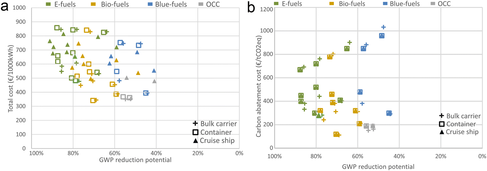 | ||
| Fig. 10 (a) Total life cycle cost against reduction of global warming potential (GWP) compared to marine gas oil (MGO) for all options for all ship types. (b) Carbon abatement cost (CAC) against reduction of global warming potential (GWP) compared to marine gas oil (MGO) for all options for all ship types. | ||
3.3 Sensitivity and scenario analysis
The cost of e-fuel, biofuels, and blue-fuel are largely affected by changes in the price of electricity, biomass, and natural gas, respectively. Therefore, in addition to the uncertainty analysis, a sensitivity analysis on selected key parameters for the different fuel production pathways is performed for the bulk carrier ICE configurations (Fig. 11). From Fig. 11b it can be observed that e-fuels can be cheaper than biofuels and blue-fuels when the electricity cost is low. Both e-ammonia and e-methanol in engines approach negative CAC when electricity prices approach zero (Fig. 11a), which shows that e-fuel can compete with fossil fuel options at very low electricity costs. Similarly, at lower biomass costs, biofuels will be the cheapest, and bio-methanol in engine approach negative CAC. However, for blue-fuels, even though natural gas costs are low, CAC is still high. This is because of the higher GWP of blue-fuels compared to other fuels.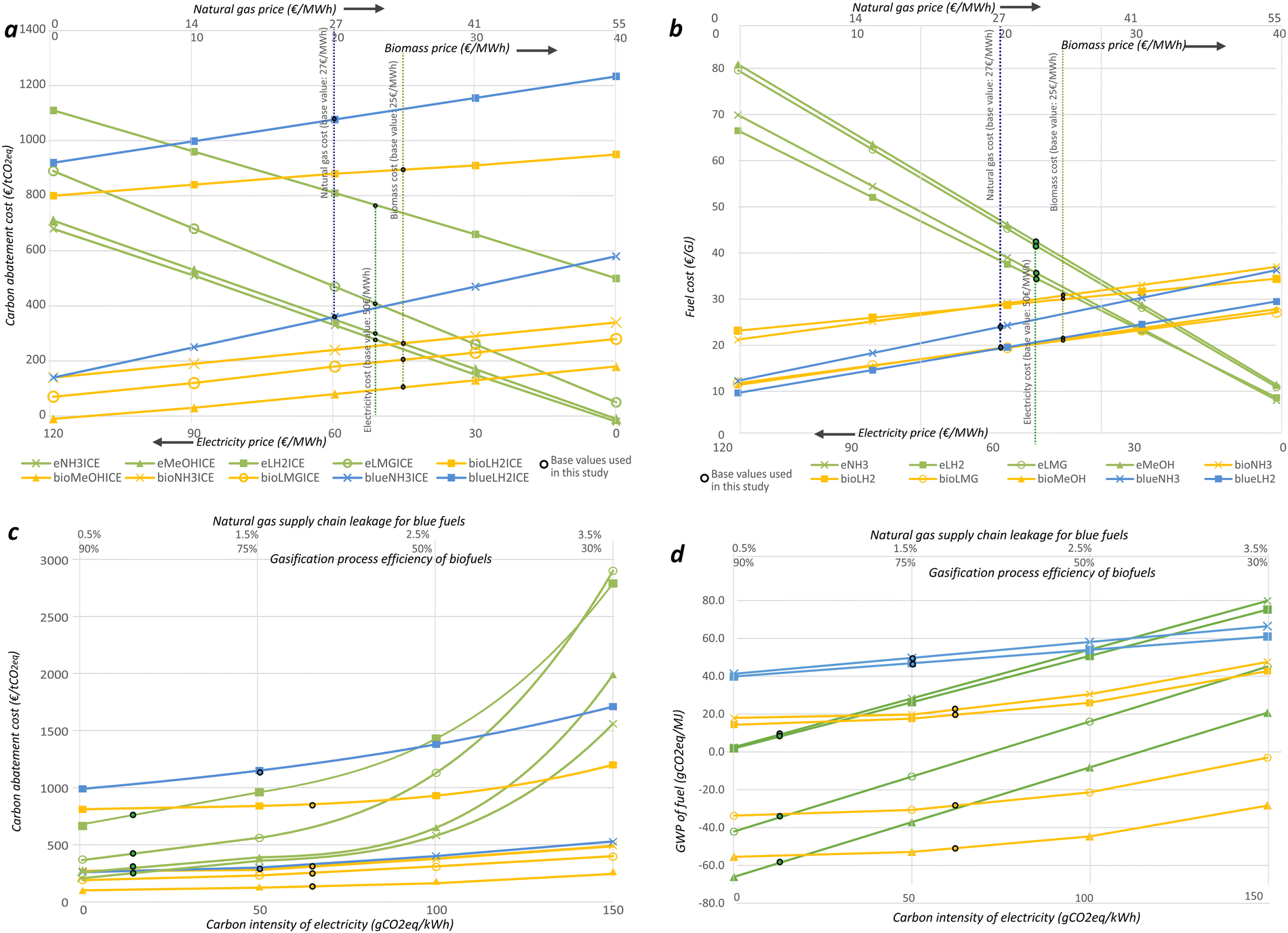 | ||
| Fig. 11 Sensitivity analysis for the bulk carrier using internal combustion engines showing (a) carbon abatement cost and (b) fuel cost as a function of electricity, biomass, and natural gas cost and (c) carbon abatement cost and (d) global warming potential based on the carbon intensity of electricity, biomass gasification efficiency and methane leakage in the natural gas supply chain. | ||
The uncertainty analysis revealed that gasification efficiency is a key parameter for biofuels, while methane leakage in natural gas is a key parameter for blue-fuels. Hence, sensitivity analyses are performed by varying methane leakage in the natural gas, biomass gasification efficiency, and the carbon intensity of the electrical mix (Fig. 11c and d). It can be noted that the carbon intensity of the electricity mix significantly influences the CAC, suggesting the need to produce e-fuels from low-carbon-intensity electricity. Furthermore, biofuels require high gasification efficiency to maintain a low CAC. Blue-fuels are highly sensitive to methane leakage from the natural gas supply chain, requiring minimal levels of methane leakage to reduce CAC.
Fig. 12 shows scenario analysis performed for the global warming potential of assessed fuel production pathways for three different SSP2 scenarios for the years 2030, 2040, 2050, and 2060. The result shows that the e-fuels produced from the electricity mix rather than wind power have a lower potential than the biofuel pathways in 2030 to reduce global warming potential. From 2040, onwards the e-fuel has a lower GWP compared to all pathways for all three scenarios. The blue fuels GWP hardly change showing that the emissions are mainly reliant on the natural gas supply and significant changes cannot be expected in the supply chain. The GWP of biofuels also reduces over time but not significantly, these are partially due to better availability of cleaner energy in processes like harvesting, collection, processing, and gasification. It may be noted that the availability of sustainable biomass supply is not evaluated.
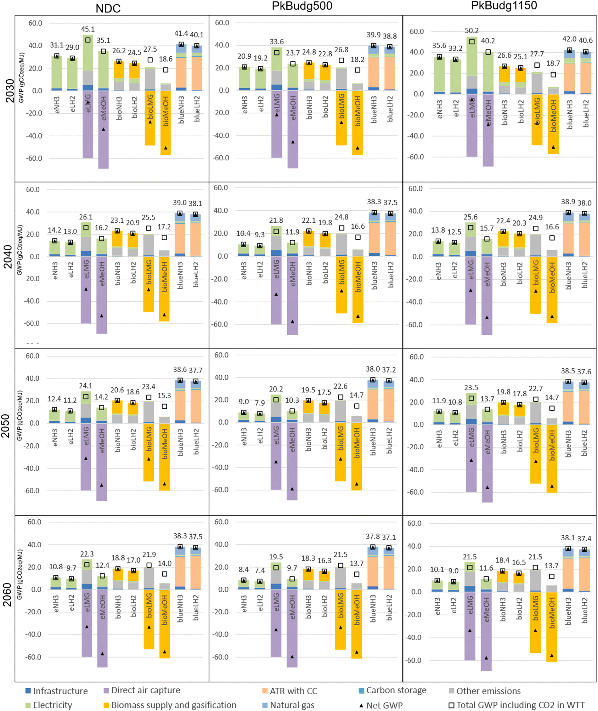 | ||
| Fig. 12 Scenario analysis of GWP for production for different fuels. Negative emission for methanol and methane is due to the presence of carbon from biogenic origin or DAC in the fuel. The scenario is given for four decades from 2030 to 2060 during the period when the case study ship will be operating. (NH3-ammonia, LH2-liquid hydrogen, LMG-liquid methane, MeOH-methanol, ATR-auto thermal reforming, CC-carbon capture, and WTT-well to tank). | ||
4. Discussions
The study focuses on the cradle-to-grave environmental and cost assessment across five main options to reduce the climate impact of shipping. The assessments are further used to calculate the carbon abatement cost to understand the cost-effectiveness of reducing GHG emissions. The results show that bio-methanol and bio-methane have a high potential for being used, as their cost projections are significantly lower than all other fuels. However, the cost is influenced by biomass costs, while the GWP is affected by the availability of sustainable biomass resources, biomass collection, and gasification efficiency. In addition, the use of biomass will create an additional environmental burden on acidification potential, land use, and eutrophication (terrestrial and freshwater). The acidification and eutrophication are due to the use of fertilizers and NOx emissions during gasification; this has also been observed in earlier studies.107,108 The high land use means that more land cover is required for producing biomass in comparison with other fuel production pathways. The availability of feedstock like biomass also depends on the geographical distribution, which will also affect WTT emissions, and it is particularly important to consider the limited availability of biomass from sustainably managed forests.109 Also, higher demand for biofuels can result in the expansion of biomass production, which can result in the emission of GHGs due to direct and indirect land use due to changes in soil carbon content and other environmental consequences like loss of biodiversity, nutrient depletion, and water consumption.29 Using biomass from non-sustainable sources will not benefit climate mitigation and will also be environmentally problematic.The results also highlight that bio-hydrogen and bio-ammonia are less promising than the other biomass routes for all ship types due to high GWP and high cost. This is due to high energy use in the production process linked to efficiency loss and the energy required for pressure swing adsorption for separating hydrogen. However, using BECCS in the production of bio-hydrogen and bio-ammonia could potentially change this result by possibly achieving negative GWP and hence reducing CAC further.46,48 A limitation of this study is that it only focuses on the gasification route for agroforestry residues. For example, the study does not consider the potential pathway of biogas from municipal solid waste.
Using e-fuels derived from wind power can significantly decrease ships' climate impact and the results show that, e-ammonia, followed by e-methanol, has the lowest CAC among e-fuels for the ship types considered. The GWP and CAC results are in line with other studies having a reduction of GWP compared to MGO in ICE greater than 85% (except for e-methane) and CAC higher than €250 € per tCO2eq.8,9,24,69 There is significant uncertainty regarding the GWP when ammonia is used in engines due to the emission of nitrous oxides, as shown in various studies.8,110 It is important to monitor and abate nitrous oxide emissions from the ammonia engines to be considered a potential decarbonization solution. E-methanol and e-methane, on the other hand, are more energy-intensive than ammonia, mainly due to CO2 from DAC. Using CO2 from biomass and waste instead of DAC and matching it with local or regional sources is another option to reduce the cost. Korberg, et al.69 considered point source biomass-based CO2 and found e-methanol cheaper than e-ammonia. When CO2 comes from a carbon capture process that delivers other products such as bioenergy plants, the impact from the process needs to be appropriately allocated between all products including CO2, unlike in a mono-functional system such as direct air capture.111 This is outside the scope of this article but is important in future assessments as biogenic CO2 sources from multifunctional systems are considered for e-fuel production.112 E-methane has the highest GWP among e-fuels due to the methane slip from the engine and fugitive emissions of methane during liquefaction and distribution. As GWP is limited and CAC is higher for e-methane options, it would be challenging for stakeholders who have already invested in ships that run on LNG.1 It may be noted that a major portion of the order book of ships is LNG-based.1 Aftertreatment technologies such as methane oxidation catalysts after treatment or plasma reduction technology can potentially be used to reduce onboard methane emissions. These are under development and have currently low service life.113 Other potential after-treatment technologies are catalysts that can be used to reduce NOx and N2O emissions. Incentives to use and further develop abatement technologies could increase with stricter regulations.
The total cost and CAC of e-fuel options are significantly influenced by the electricity price, which varies significantly across different regions. Utilizing an electricity mix with carbon intensity instead of wind power also leads to increased GWP and CAC for e-fuel options. Not all regions have access to low climate-impact electricity; investments in renewable electricity sources are critical for increasing the potential use of e-fuels in the shipping sector. On the downside, e-fuels produced using electricity from wind power will have an increased impact on human toxicity and resource use due to materials such as copper, zinc, and rare-earths, in addition to steel in wind power infrastructure and electrolyzers. The environmental burden from the materials used in wind power infrastructure and electrolyzers can be reduced by recycling or reusing the materials and also by using materials produced from cleaner technologies, like fossil-free steel.9
A lower fuel cost makes blue-ammonia and blue-hydrogen options more cost-effective overall compared to e-based and bio-based alternatives; however, the higher GWP results in higher CAC costs. This indicates that blue-fuels can be competitive from a cost perspective with e-fuels but have limited climate reduction potential and are not sufficient to meet the long-term IMO GHG reduction target. Another challenge for blue-fuels is that environmental burdens are shifted from the TTW to the WTT (i.e., fuel production), and there are increased environmental impacts on categories like fossil resource use (due to the additional energy required for steam methane reforming in the WTT) and acidification potential (from flue gas in the steam methane reformer). Methane leakage in the natural gas supply chain and the carbon capture rate are important parameters that determine the GWP for blue-fuel options. Currently, methane leakage from the supply chain ranges from less than 0.5% to over 2.5%, depending on the geographical location.65,114 CAC of the blue-fuel options relies on a low-cost natural gas supply with low greenhouse gas emissions, which requires minimizing methane leaks and emissions across the entire supply chain. OCC performs better compared to blue-fuels and has one of the lowest CACs of all technological options. Similar to blue-fuels, the climate impact reduction possibility is limited by the carbon capture rate and also by the energy penalty required for operating the carbon capture system onboard and CO2 liquefaction. However, the OCC has a higher environmental burden (excluding climate change) over the life cycle than the reference MGO case due to the energy penalty for the operation of the carbon capture system onboard. The availability of a port reception facility and CO2 transport, as well as the proximity to the permanent storage site, is another significant challenge that should be addressed for the OCC.115,116 Also, the operation of OCC reduces the availability of heat for other purposes on board ships, like space heating, which will have a greater effect on passenger ships. Our study shows the carbon abatement cost is higher than 150 € per tCO2eq, whereas most of the different studies indicate a wide range of carbon removal costs using OCC, from 85 to 149 € per tCO2115,117 whereas some studies show it can be higher than 200 € per tCO2.32
Battery electric options are irrelevant for these long-range ships, as long as no radical technological advances or system changes are emerging,28 from both a techno-economic and an environmental point of view. The major impact comes from the higher energy storage requirement between bunkering, which determines the capacity of batteries onboard. This is also critical for low volumetric energy density carriers like liquid hydrogen, where the tank has a higher impact on both the cost and environmental performance of the pathway. For ships operating on long routes like these case study ships, liquid hydrogen options won't be a viable choice in terms of environmental and cost performance. The infrastructure needed for the storage and bunkering of liquid hydrogen at ports is another significant factor affecting the competitiveness of this fuel and there is currently limited knowledge about the cost and environmental performance of large-scale hydrogen bunkering infrastructure.118 The total cost of fuel cell options is higher for all types of ships because of the higher investment cost and the shorter life of fuel cells. However, the CAC of fuel cells is dependent on the type of ship and its operational profile. For example, among the case study ships, fuel cell options have a lower CAC than ICE options for the same fuel for cruise ships. FC options can have a lower CAC than ICE options for the same fuel when the utilization rate is high, which refers to higher annual energy use per installed capacity, as mentioned in earlier studies.9,69 The high investment cost and limited lifespan of fuel cells pose significant limitations when considering the adoption of fuel cell technology. However, improvements in these key elements can make a significant change in competitiveness due to the higher efficiency and cleaner combustion that fuel cells offer.
One of the limitations of the study is the selection of the functional unit as the maximum transport work instead of actual transport work. This assumption overestimates the capacity loss (transport loss), as often the actual transport work is less than the maximum transport work. On the other hand, the extra weight of the new propulsion system and tanks can result in increased draught and increased hull resistance. This increased resistance would have an impact on energy use for the same operational parameters. The main reason for not considering both of the above effects is the uncertainty surrounding the required tank size, as existing ships often have oversized tanks that are not aligned with the transport missions. The design of the tanks would also modify the operational behavior of ships, with more focus on design range based on speed and route. More information on the transport mission would be required for modeling behavior and, hence, tank size and capacity. Feasibility studies about changes in transport work are performed in other studies,9,24 however, these studies also have not considered it from a life cycle perspective. Another limitation of this study is also that climate impacts due to hydrogen leakage in the supply chain are not considered, even as research indicates that the indirect global warming potential of hydrogen is not negligible.55 We did not explore the geographical position of the port of operation for these ships, which could impact the cost and availability of feedstock for fuel production. The availability of feedstock influences the fuel supply and demand, which in turn affects the accessibility of new fuels at the ship's operating ports which is critical for the implementation. Additionally, it must ensure that the fuel type remains consistent for the same ship at all ports of operation, irrespective of the production pathway.
5. Conclusions
This study investigated the environmental impact, economic performance, and carbon abatement cost of 23 decarbonization pathways for three ship types. The findings highlight the critical role of the fuel production pathways in achieving emissions reductions. Among biofuels from gasification, methanol and to some extent methane are more favorable than ammonia and hydrogen, while ammonia and methanol are particularly desirable options among e-fuels. The result shows that battery electric options are not viable for long-range shipping from both environmental and cost perspectives and liquid hydrogen is also not promising from the cost perspective. Blue-fuels offer limited effectiveness in reducing climate impact and have a higher environmental footprint, but they have lower fuel costs compared to e-fuel and biofuel alternatives. Onboard carbon capture technologies have low cost and low carbon abatement cost of around 150–190 € per tCO2eq. Overall the most promising fuel is bio-methanol with carbon abatement cost between 110–120 € per tCO2eq and the lowest life cycle cost. However, prioritizing sustainable biomass sources and maximizing gasification efficiency are crucial to minimizing biofuels’ environmental footprint.Biofuels hold strategic importance for the shipping sector's timely achievement of emission targets. However, the availability of biomass from sustainable sources is limited. Additionally, competition from other sectors demanding biofuels could significantly impact biomass prices. Implementing biofuels in shipping effectively requires sector-specific policies like subsidies and rebates. Moreover, the implementation of agricultural regulations and practices is also required to ensure the mobilization of sustainable biomass. Blue-fuels and onboard carbon capture options are insufficient to achieve the 2050 greenhouse gas emission reduction targets and present limited environmental sustainability. The policy support for these options needs to consider that they are short-term transition solutions. It is highly unlikely that e-fuels will be competitive in the short term. The future of e-fuels depends on the capacity development of renewable energy production, as abatement costs depend on both lower electricity costs and the availability of renewable electricity. This implies that bridging the gap between fossil fuels and e-fuels needs specific policy support for fuel producers and ship owners. E-fuels have the potential to become a long-term backup technology: if the electricity cost reaches below a threshold and also with carbon price reaches a certain threshold, e-fuels could completely replace fossil fuels and also decrease the dependence on less sustainable alternatives like blue-fuels, or onboard carbon capture technologies.
Data availability
The data supporting this article have been included as part of the ESI.†Conflicts of interest
There are no conflicts of interest to declare.Acknowledgements
The research was performed within the project ‘Nordic Roadmap for the introduction of sustainable zero-carbon fuels in shipping” funded by Nordic council of Ministers, the project ‘FEMAR’ funded by the Swedish Transport Administration (grant number 2022/107506) and the project Hydrogen Engine Emissions Reduction (HEER) (grant number P2020-90081) funded by the Swedish Energy Agency.References
- UNCTD, Review of Maritime Transport 2022, United Nations, New York, ISBN: 978-92-1-113073-7, 2022.
- International Maritime Organization, Reduction of GHG emissions from Ships: Fourth IMO GHG Study 2020, International Maritime Organization, London, 2021.
- H. Liu,
et al., Emissions and health impacts from global shipping embodied in US–China bilateral trade, Nat. Sustainability, 2019, 2(11), 1027–1033, DOI:10.1038/s41893-019-0414-z
.
-
K. Andersson, S. Brynolf, F. Lindgren and M. Wilewska-Bien, Shipping and the Environment: Improving Environmental Performance in Marine Transportation, Springer Berlin Heidelberg, Berlin, Heidelberg: Imprint: Springer, 1st edn, 2016, p. 1 online resource (XXIII), 426 pages 77 illustrations, 49 illustrations in color Search PubMed
- M. O. P. Ramacher,
et al., The impact of ship emissions on air quality and human health in the Gothenburg area – Part II: Scenarios for 2040, Atmos. Chem. Phys., 2020, 20(17), 10667–10686, DOI:10.5194/acp-20-10667-2020
- IMO, Marine Environment Protection Committee (MEPC), https://www.imo.org/en/MediaCentre/MeetingSummaries/Pages/MEPC-default.aspx (accessed 10 Jul, 2023).
-
The European Council, Fit for 55: deal on new EU rules for cleaner maritime fuels, ed. G. Vilkas, The European Council, 2023 Search PubMed
- F. M. Kanchiralla, S. Brynolf, E. Malmgren, J. Hansson and M. Grahn, Life-Cycle Assessment and Costing of Fuels and Propulsion Systems in Future Fossil-Free Shipping, Environ. Sci. Technol., 2022, 56(17), 12517–12531, DOI:10.1021/acs.est.2c03016
- F. M. Kanchiralla, S. Brynolf, T. Olsson, J. Ellis, J. Hansson and M. Grahn, How do variations in ship operation impact the techno-economic feasibility and life cycle environmental performance of fossil-free fuels? a life cycle study, Appl. Energy, 2023, 350 DOI:10.1016/j.apenergy.2023.121773
- E. Malmgren, S. Brynolf, E. Fridell, M. Grahn and K. Andersson, The environmental performance of a fossil-free ship propulsion system with onboard carbon capture–a life cycle assessment of the HyMethShip concept, Sustainable Energy Fuels, 2021, 5(10), 2753–2770 RSC
- S. Brynolf, E. Fridell and K. Andersson, Environmental assessment of marine fuels: liquefied natural gas, liquefied biogas, methanol and bio-methanol, (in English), J. Cleaner Prod., 2014, 74, 86–95, DOI:10.1016/j.jclepro.2014.03.052
- N. de Fournas and M. Wei, Techno-economic assessment of renewable methanol from biomass gasification and PEM electrolysis for decarbonization of the maritime sector in California, Energy Convers. Manage., 2022, 257, 115440, DOI:10.1016/j.enconman.2022.115440
- P. Gilbert, C. Walsh, M. Traut, U. Kesieme, K. Pazouki and A. Murphy, Assessment of full life-cycle air emissions of alternative shipping fuels, J. Cleaner Prod., 2018, 172, 855–866, DOI:10.1016/j.jclepro.2017.10.165
- T. R. Hawkins, U. Lee, M. Wang and T. Thompson, Life Cycle Assessment of Greenhouse Gas and Criteria Air Pollutant Emissions from Conventional and Biobased Marine Fuels, U.S. DEPARTMENT OF TRANSPORTATION, Maritime Administration, Washington, 2019. [Online]. Available: https://www.maritime.dot.gov/innovation/meta/life-cycle-assessment-greenhouse-gas-and-criteria-air-pollutant-emissions.
- L. C. Law, B. Foscoli, E. Mastorakos and S. Evans, A comparison of alternative fuels for shipping in terms of lifecycle energy and cost, Energies, 2021, 14(24), 8502 CrossRef CAS
- G. Horton, et al., Technological, Operational and Energy Pathways for Maritime Transport to Reduce Emissions Towards 2050. Final report. Report for OGCI/Concawe, Ricardo, Didcot, UK, 2022.
- E. C. D. Tan,
et al., Biofuel Options for Marine Applications: Technoeconomic and Life-Cycle Analyses, Environ. Sci. Technol., 2021, 55(11), 7561–7570, DOI:10.1021/acs.est.0c06141
- S. E. Tanzer, J. Posada, S. Geraedts and A. Ramírez, Lignocellulosic marine biofuel: Technoeconomic and environmental assessment for production in Brazil and Sweden, J. Cleaner Prod., 2019, 239, 117845, DOI:10.1016/j.jclepro.2019.117845
- D. M. M. Yacout, M. Tysklind and V. K. K. Upadhyayula, Assessment of forest-based biofuels for Arctic marine shipping, Resour., Conserv. Recycl., 2021, 174, 105763, DOI:10.1016/j.resconrec.2021.105763
- Y. Zhou, N. Pavlenko, D. Rutherford, L. Osipova and B. Comer, The potential of liquid biofuels in reducing ship emissions. ICCT WORKING PAPER 2020-21, International Council on Clean Transportation, 2020.
- L. Bilgili, Comparative assessment of alternative marine fuels in life cycle perspective, Renewable Sustainable Energy Rev., 2021, 144, 110985, DOI:10.1016/j.rser.2021.110985
- S. Brynolf, M. Taljegard, M. Grahn and J. Hansson, Electrofuels for the transport sector: a review of production costs, Renewable Sustainable Energy Rev., 2018, 81, 1887–1905, DOI:10.1016/j.rser.2017.05.288
- E. Lindstad, B. Lagemann, A. Rialland, G. M. Gamlem and A. Valland, Reduction of maritime GHG emissions and the potential role of E-fuels, Trans. Res., Part D: Trans. Environ., 2021, 101 DOI:10.1016/j.trd.2021.103075
- B. Stolz, M. Held, G. Georges and K. Boulouchos, Techno-economic analysis of renewable fuels for ships carrying bulk cargo in Europe, Nat. Energy, 2022, 7(2), 203–212, DOI:10.1038/s41560-021-00957-9
- H. Xing, C. Stuart, S. Spence and H. Chen, Alternative fuel options for low carbon maritime transportation: Pathways to 2050, J. Cleaner Prod., 2021, 297 DOI:10.1016/j.jclepro.2021.126651
- M. Percic, I. Ancic and N. Vladimir, Life-cycle cost assessments of different power system configurations to reduce the carbon footprint in the Croatian short-sea shipping sector, (in English), Renewable Sustainable Energy Rev., 2020, 131 DOI:10.1016/j.rser.2020.110028
- M. Perčić, N. Vladimir and A. Fan, Life-cycle cost assessment of alternative marine fuels to reduce the carbon footprint in short-sea shipping: a case study of Croatia, Appl. Energy, 2020, 279 DOI:10.1016/j.apenergy.2020.115848
- J. Kersey, N. D. Popovich and A. A. Phadke, Rapid battery cost declines accelerate the prospects of all-electric interregional container shipping, Nat. Energy, 2022, 7(7), 664–674, DOI:10.1038/s41560-022-01065-y
- H. K. Jeswani, A. Chilvers and A. Azapagic, Environmental sustainability of biofuels: a review, Proc. R. Soc. A, 2020, 476(2243), 20200351, DOI:10.1098/rspa.2020.0351
-
F. M. Kanchiralla, Life cycle navigation through future energy carriers and propulsion options for the energy transition in shipping, Licentiate of Engineering Licentiate, Department of Mechanics and Maritime Sciences, Chalmers University of Technology, Gothenburg, Sweden, Technical report no 2023:05., 2023 Search PubMed
- L. J. Müller, A. Kätelhön, M. Bachmann, A. Zimmermann, A. Sternberg and A. Bardow, A Guideline for Life Cycle Assessment of Carbon Capture and Utilization, Front. Energy Res., 2020, 8 DOI:10.3389/fenrg.2020.00015
- M. Feenstra, J. Monteiro, J. T. van den Akker, M. R. M. Abu-Zahra, E. Gilling and E. Goetheer, Ship-based carbon capture onboard of diesel or LNG-fuelled ships, Int. J. Greenhouse Gas Control, 2019, 85, 1–10, DOI:10.1016/j.ijggc.2019.03.008
- S. Lee, S. Yoo, H. Park, J. Ahn and D. Chang, Novel methodology for EEDI calculation considering onboard carbon capture and storage system, Int. J. Greenhouse Gas Control, 2021, 105 DOI:10.1016/j.ijggc.2020.103241
- A. Mjelde, K. Martinsen, M. Eide and O. Endresen, Environmental accounting for Arctic shipping – a framework building on ship tracking data from satellites, Mar. Pollut. Bull., 2014, 87(1–2), 22–28, DOI:10.1016/j.marpolbul.2014.07.013
- DNVAS, Maritime Forecast to 2050 – Energy Transition Outlook 2019, DNV GL., 2019. [Online]. Available: https://www.dnv.com/energy-transition-outlook/index.html.
- S. Brynolf, et al., Nordic Roadmap Publication No. 1-C/1/2022, 2022.
- S. A. Nosherwani and R. C. Neto, Techno-economic assessment of commercial ammonia synthesis methods in coastal areas of Germany, J. Energy Storage, 2021, 34 DOI:10.1016/j.est.2020.102201
- A. Sternberg and A. Bardow, Life Cycle Assessment of Power-to-Gas: Syngas vs Methane, ACS Sustainable Chem. Eng., 2016, 4(8), 4156–4165, DOI:10.1021/acssuschemeng.6b00644
- S. Deutz and A. Bardow, Life-cycle assessment of an industrial direct air capture process based on temperature–vacuum swing adsorption, Nat. Energy, 2021, 6(2), 203–213, DOI:10.1038/s41560-020-00771-9
- G. Amaya-Santos, S. Chari, A. Sebastiani, F. Grimaldi, P. Lettieri and M. Materazzi, Biohydrogen: A life cycle assessment and comparison with alternative low-carbon production routes in UK, J. Cleaner Prod., 2021, 319 DOI:10.1016/j.jclepro.2021.128886
- IEA, Net Zero Roadmap: A Global Pathway to Keep the 1.5 °C Goal in Reach, International Energy Agency, Paris, 2023.
- IRENA, Global Bioenergy supply and demand projections for the Year 2030, International Renewable Energy Agency, Abu Dhabi, 2014.
- A. Thorenz, L. Wietschel, D. Stindt and A. Tuma, Assessment of agroforestry residue potentials for the bioeconomy in the European Union, J. Cleaner Prod., 2018, 176, 348–359, DOI:10.1016/j.jclepro.2017.12.143
- B. Rijal, S. H. Gautam and L. LeBel, The impact of forest disturbances on residual biomass supply: a long-term forest level analysis, J. Cleaner Prod., 2020, 248 DOI:10.1016/j.jclepro.2019.119278
- S. E. Tanzer, J. Posada, S. Geraedts and A. Ramírez, Lignocellulosic marine biofuel: Technoeconomic and environmental assessment for production in Brazil and Sweden, J. Cleaner Prod., 2019, 239 DOI:10.1016/j.jclepro.2019.117845
- C. Antonini, K. Treyer, E. Moioli, C. Bauer, T. J. Schildhauer and M. Mazzotti, Hydrogen from wood gasification with CCS – a techno-environmental analysis of production and use as transport fuel, Sustainable Energy Fuels, 2021, 5(10), 2602–2621, 10.1039/d0se01637c
- S. C. Galusnyak, L. Petrescu, D. A. Chisalita, C.-C. Cormos and M. Ugolini, From Secondary Biomass to Bio-Methanol through CONVERGE Technology: An Environmental Analysis, Energies, 2023, 16(6) DOI:10.3390/en16062726
- S. C. D’Angelo,
et al., Planetary Boundaries Analysis of Low-Carbon Ammonia Production Routes, ACS Sustainable Chem. Eng., 2021, 9(29), 9740–9749, DOI:10.1021/acssuschemeng.1c01915
- C. Antonini, K. Treyer, A. Streb, M. van der Spek, C. Bauer and M. Mazzotti, Hydrogen production from natural gas and biomethane with carbon capture and storage – A techno-environmental analysis, Sustainable Energy Fuels, 2020, 4(6), 2967–2986, 10.1039/d0se00222d
-
F. M. Kanchiralla, S. Brynolf, E. Malmgren and M. Grahn, Can Shipping Contribute to Negative CO2 Emissions?, 2nd International Conference on Negative CO2 Emissions, Göteborg, Sweden, 2022, pp. 14–17 Search PubMed
- B. Thaler,
et al., Optimal design and operation of maritime energy systems based on renewable methanol and closed carbon cycles, Energy Convers. Manage., 2022, 269 DOI:10.1016/j.enconman.2022.116064
- ISO 14044: 2006, Environmental management—Life cycle assessment, International Organization for Standardization, 2006.
- S. Cucurachi, C. van der Giesen and J. Guinée, Ex-ante LCA of Emerging Technologies, Proc. CIRP, 2018, 69, 463–468, DOI:10.1016/j.procir.2017.11.005
- IEA, World energy outlook 2022, International Energy Agency, Paris, 2022.
- R. G. Derwent, Global warming potential (GWP) for hydrogen: Sensitivities, uncertainties and meta-analysis, Int. J. Hydrogen Energy, 2023, 48(22), 8328–8341, DOI:10.1016/j.ijhydene.2022.11.219
- J. Q. Mathieu Delpierre, Jan Mertens, Anne Prieur-Vernat and Stefano Cucurachi, Assessing the environmental impacts of wind-based hydrogen production in the Netherlands using ex-ante LCA and scenarios analysis, J. Cleaner Prod., 2021, 299 CrossRef
- Danish Energy Agency, Technology data for renewable fuels. Updated July 2020, Copenhagen, 2017.
- A. Lotrič, M. Sekavčnik, I. Kuštrin and M. Mori, Life-cycle assessment of hydrogen technologies with the focus on EU critical raw materials and end-of-life strategies, Int. J. Hydrogen Energy, 2021, 46(16), 10143–10160, DOI:10.1016/j.ijhydene.2020.06.190
- C. Smith, A. K. Hill and L. Torrente-Murciano, Current and future role of Haber–Bosch ammonia in a carbon-free energy landscape, Energy Environ. Sci., 2020, 13(2), 331–344, 10.1039/c9ee02873k
- G. Wernet, C. Bauer, B. Steubing, J. Reinhard, E. Moreno-Ruiz and B. Weidema, The ecoinvent database version 3 (part I): overview and methodology, Int. J. Life Cycle Assess., 2016, 21(9), 1218–1230, DOI:10.1007/s11367-016-1087-8
- A. A. Kiss, J. J. Pragt, H. J. Vos, G. Bargeman and M. T. de Groot, Novel efficient process for methanol synthesis by CO 2 hydrogenation, Chem. Eng. J., 2016, 284, 260–269, DOI:10.1016/j.cej.2015.08.101
- Y. Gu, D. Wang, Q. Chen and Z. Tang, Techno-economic analysis of green methanol plant with optimal design of renewable hydrogen production: A case study in China, Int. J. Hydrogen Energy, 2022, 47(8), 5085–5100, DOI:10.1016/j.ijhydene.2021.11.148
- K. Stolzenburg and R. Mubbala, Integrated Design for Demonstration of Efficient Liquefaction of Hydrogen (IDEALHY Deliverable 3.16), Fuel Cells and Hydrogen Joint Undertaking (FCH JU), 16 December 2013.
- M. Grahn,
et al., Review of electrofuel feasibility—cost and environmental impact, Prog. Energy, 2022, 4(3), 032010, DOI:10.1088/2516-1083/ac7937
- P. Balcombe, K. Anderson, J. Speirs, N. Brandon and A. Hawkes, The Natural Gas Supply Chain: The Importance of Methane and Carbon Dioxide Emissions, ACS Sustainable Chem. Eng., 2016, 5(1), 3–20, DOI:10.1021/acssuschemeng.6b00144
- A. Susmozas, D. Iribarren and J. Dufour, Life-cycle performance of indirect biomass gasification as a green alternative to steam methane reforming for hydrogen production, Int. J. Hydrogen Energy, 2013, 38(24), 9961–9972, DOI:10.1016/j.ijhydene.2013.06.012
- C. Lodato, L. Hamelin, D. Tonini and T. F. Astrup, Towards sustainable methane supply from local bioresources: Anaerobic digestion, gasification, and gas upgrading, Appl. Energy, 2022, 323 DOI:10.1016/j.apenergy.2022.119568
- Danish Energy Agency, Technology Data – Carbon Capture, Transport and Storage, November 2021, Copenhagen, 2021.
- A. D. Korberg, S. Brynolf, M. Grahn and I. R. Skov, Techno-economic assessment of advanced fuels and propulsion systems in future fossil-free ships, (in English), Renewable Sustainable Energy Rev., 2021, 142 DOI:10.1016/j.rser.2021.110861
- M. Al-Breiki and Y. Bicer, Technical assessment of liquefied natural gas, ammonia and methanol for overseas energy transport based on energy and exergy analyses, Int. J. Hydrogen Energy, 2020, 45(60), 34927–34937, DOI:10.1016/j.ijhydene.2020.04.181
- G. Parks, R. Boyd, J. Cornish and R. Remick, Hydrogen Station Compression, Storage, and Dispensing: Technical Status and Costs, Technical Report NREL/BK-6A10-58564, 2014.
- E. Malmgren, S. Brynolf, E. Fridell, M. Grahn and K. Andersson, The environmental performance of a fossil-free ship propulsion system with onboard carbon capture – a life cycle assessment of the HyMethShip concept, Sustainable Energy Fuels, 2021, 5, 2753–2770, 10.1039/D1SE00105A
- K. P. Jain, J. F. J. Pruyn and J. J. Hopman, Quantitative assessment of material composition of end-of-life ships using onboard documentation, Resour., Conserv. Recycl., 2016, 107, 1–9, DOI:10.1016/j.resconrec.2015.11.017
- B. Jeong, H. Wang, E. Oguz and P. Zhou, An effective framework for life cycle and cost assessment for marine vessels aiming to select optimal propulsion systems, J. Cleaner Prod., 2018, 187, 111–130, DOI:10.1016/j.jclepro.2018.03.184
- Diesel Electric Propulsion plant, Man Energy solutions.
-
M. I. Battelle, Manufacturing Cost Analysis of PEM Fuel Cell Systems for 5- and 10-kW Backup Power Applications, Columbus, 2016 Search PubMed
- L. Usai, C. R. Hung, F. Vasquez, M. Windsheimer, O. S. Burheim and A. H. Stromman, Life cycle assessment of fuel cell systems for light duty vehicles, current state-of-the-art and future impacts, J. Cleaner Prod., 2021, 280, 125086, DOI:10.1016/j.jclepro.2020.125086
- K. Al-Khori, S. G. Al-Ghamdi, S. Boulfrad and M. Koç, Life Cycle Assessment for Integration of Solid Oxide Fuel Cells into Gas Processing Operations, Energies, 2021, 14(15) DOI:10.3390/en14154668
- S. Grzesiak, Alternative Propulsion Plants for Modern LNG Carriers, New Trends Prod. Eng., 2018, 1(1), 399–407, DOI:10.2478/ntpe-2018-0050
- Interrag, Danube Transnational Program-Grendel, DST – Development Centre for Ship Technology and Transport Systems, 2020.
- Element Energy Limited, Shipping CO2 – UK Cost estimation study, Business, Energy & Industrial Strategy Department, Cambridge, 2018.
- L. Giordano, D. Roizard and E. Favre, Life cycle assessment of post-combustion CO2 capture: a comparison between membrane separation and chemical absorption processes, Int. J. Greenhouse Gas Control, 2018, 68, 146–163, DOI:10.1016/j.ijggc.2017.11.008
-
L. Irlam, Global costs of carbon capture and storage, Global CCS institute, Melbourne, 2017 Search PubMed
- J. A. Ros,
et al., Advancements in ship-based carbon capture technology on board of LNG-fuelled ships, Int. J. Greenhouse Gas Control, 2022, 114 DOI:10.1016/j.ijggc.2021.103575
- R. Kleijn, E. van der Voet, G. J. Kramer, L. van Oers and C. van der Giesen, Metal requirements of low-carbon power generation, Energy, 2011, 36(9), 5640–5648, DOI:10.1016/j.energy.2011.07.003
- Siemens: Sigentics M generators Catalogue, PDLD-B10133-00-7600, 2018. [Online]. Available: siemens.com/sigentics-m.
- GREET Database.
- K. Kim, G. Roh, W. Kim and K. Chun, A Preliminary Study on an Alternative Ship Propulsion System Fueled by Ammonia: Environmental and Economic Assessments, J. Marine Sci. Eng., 2020, 8(3) DOI:10.3390/jmse8030183
-
Department of Transport, Clean Maritime Plan, Department of Transport, London, 2019 Search PubMed
- Z. Liang, X. Ma, H. Lin and Y. Tang, The energy consumption and environmental impacts of SCR technology in China, Appl. Energy, 2011, 88(4), 1120–1129, DOI:10.1016/j.apenergy.2010.10.010
- M. Wentker, M. Greenwood and J. Leker, A Bottom-Up Approach to Lithium-Ion Battery Cost Modeling with a Focus on Cathode Active Materials, Energies, 2019, 12(3) DOI:10.3390/en12030504
- F. Ueckerdt, C. Bauer, A. Dirnaichner, J. Everall, R. Sacchi and G. Luderer, Potential and risks of hydrogen-based e-fuels in climate change mitigation, Nat. Clim. Change, 2021, 11(5), 384–393, DOI:10.1038/s41558-021-01032-7
- M. Chordia, A. Nordelöf and L. A.-W. Ellingsen, Environmental life cycle implications of upscaling lithium-ion battery production, Int. J. Life Cycle Assess., 2021, 26 DOI:10.1007/s11367-021-01976-0
- L. A.-W. Ellingsen, G. Majeau-Bettez, B. Singh, A. K. Srivastava, L. O. Valøen and A. H. Strømman, Life Cycle Assessment of a Lithium-Ion Battery Vehicle Pack, J. Ind. Ecol., 2014, 18(1), 113–124, DOI:10.1111/jiec.12072
- IPCC 2021, Climate Change 2021: The Physical Science Basis. Sixth Assessment Report of the Intergovernmental Panel on Climate Change, Cambridge University Press, Cambridge, United Kingdom and New York, NY, USA, pp. 2391 DOI:10.1017/9781009157896.2021.
-
L. Zampori and P. Rana, Suggestions for updating the Product Environmental Footprint (PEF) method, EUR 29682 EN, Luxembourg, 2019 Search PubMed
- E. Crenna, M. Secchi, L. Benini and S. Sala, Global environmental impacts: data sources and methodological choices for calculating normalization factors for LCA, Int. J. Life Cycle Assess., 2019, 24(10), 1851–1877, DOI:10.1007/s11367-019-01604-y
- S. Sala, E. Crenna, M. Secchi and R. Pant, Global normalisation factors for the environmental footprint and life cycle assessment, European Commission, Joint Research Centre, ISBN 978-92-79-77213-9, 2017.
-
S. Sala, A. Kim Cerutti and R. Pant, Development of a weighting approach for the Environmental Footprint, European Commission, Joint Research Centre, ISBN 978-92-79-68042-7, 2018 Search PubMed
- Frontier Economics, CO2 emission abatement costs of gas mobility and other road transport options: Report for NGVA Europe, London, April 2021.
- K. Riahi,
et al., The Shared Socioeconomic Pathways and their energy, land use, and greenhouse gas emissions implications: An overview, Global Environ. Change, 2017, 42, 153–168, DOI:10.1016/j.gloenvcha.2016.05.009
- R. Sacchi,
et al., PRospective EnvironMental Impact asSEment (premise): A streamlined approach to producing databases for prospective life cycle assessment using integrated assessment models, Renewable Sustainable Energy Rev., 2022, 160 DOI:10.1016/j.rser.2022.112311
- L. Baumstark,
et al., REMIND2.1: transformation and innovation dynamics of the energy-economic system within climate and sustainability limits, Geosci. Model Dev., 2021, 14(10), 6571–6603, DOI:10.5194/gmd-14-6571-2021
- R. Besseau, R. Sacchi, I. Blanc and P. Pérez-López, Past, present and future environmental footprint of the Danish wind turbine fleet with LCA_WIND_DK, an online interactive platform, Renewable Sustainable Energy Rev., 2019, 108, 274–288, DOI:10.1016/j.rser.2019.03.030
- C. Panoutsou,
et al., Advanced biofuels to decarbonise European transport by 2030: Markets, challenges, and policies that impact their successful market uptake, Energy Strategy Rev., 2021, 34 DOI:10.1016/j.esr.2021.100633
- V. Daioglou,
et al., Greenhouse gas emission curves for advanced biofuel supply chains, Nat. Clim. Change, 2017, 7(12), 920–924, DOI:10.1038/s41558-017-0006-8
- M. Costa, D. Piazzullo, D. Di Battista and A. De Vita, Sustainability assessment of the whole biomass-to-energy chain of a combined heat and power plant based on biomass gasification: biomass supply chain management and life cycle assessment, J. Environ. Manage., 2022, 317, 115434, DOI:10.1016/j.jenvman.2022.115434
- G. Zang, J. Zhang, J. Jia, E. S. Lora and A. Ratner, Life cycle assessment of power-generation systems based on biomass integrated gasification combined cycles, Renewable Energy, 2020, 149, 336–346, DOI:10.1016/j.renene.2019.12.013
-
European Commission, Development of outlook for the necessary means to build industrial capacity for drop-in advanced biofuels, Luxembourg, 2024 Search PubMed
- A. Kumar, K. Kamasamudram, N. Currier and A. Yezerets, SCR Architectures for Low N2O Emissions, SAE Tech. Pap. Ser. 2015-01-1030, 2015 DOI:10.4271/2015-01-1030
- N. von der Assen, J. Jung and A. Bardow, Life-cycle assessment of carbon dioxide capture and utilization: avoiding the pitfalls, Energy Environ. Sci., 2013, 6(9) 10.1039/c3ee41151f
- Liquid wind. eMethanol-A fossil-free liquid eFuel. https://www.liquidwind.se/emethanol (accessed 05 April, 2024).
- Maersk Mc-Kinney Møller Center for Zero Carbon Shipping, Reducing methane emissions onboard vessels, 2022.
- C. Bauer,
et al., On the climate impacts of blue hydrogen production, Sustainable Energy Fuels, 2022, 6(1), 66–75, 10.1039/d1se01508g
- V. Negri, M. A. Charalambous, J. D. Medrano-Garcia and G. Guillen-Gosalbez, Navigating within the Safe Operating Space with Carbon Capture On-Board, ACS Sustainable Chem. Eng., 2022, 10(51), 17134–17142, DOI:10.1021/acssuschemeng.2c04627
- M. Buirma, J. Vleugel, J. Pruyn, V. Doedée and D. Schott, Ship-Based Carbon Capture and Storage: A Supply Chain Feasibility Study, Energies, 2022, 15(3) DOI:10.3390/en15030813
- A. Awoyomi, K. Patchigolla and E. J. Anthony, Process and Economic Evaluation of an Onboard Capture System for LNG-Fueled CO2 Carriers, Ind. Eng. Chem. Res., 2019, 59(15), 6951–6960, DOI:10.1021/acs.iecr.9b04659
- L. Van Hoecke, L. Laffineur, R. Campe, P. Perreault, S. W. Verbruggen and S. Lenaerts, Challenges in the use of hydrogen for maritime applications, Energy Environ. Sci., 2021, 14(2), 815–843, 10.1039/d0ee01545h
Footnote |
| † Electronic supplementary information (ESI) available. See DOI: https://doi.org/10.1039/d4ee01641f |
| This journal is © The Royal Society of Chemistry 2024 |