A tutorial review of linear rheology for polymer chemists: basics and best practices for covalent adaptable networks

Abstract

Covalent adaptable networks (CANs) are an emerging class of soft materials that combine the contradictory traits of thermosets and thermoplastics. They possess dynamic covalent cross-links between chains that exchange through a chemical reaction. Because the flow behavior of CANs reflects the interplay between the cross-link exchange kinetics and polymer backbone dynamics, careful rheological characterization is necessary to illuminate how chemical structure governs viscoelasticity. Yet, rheology presents a significant challenge for polymer chemists as an analytical technique because of the complexity of the measurement and data analysis. Considering the prevalence and significance of rheology in the field of soft matter, however, it is essential for modern polymer chemists to possess a foundation in conducting and interpreting viscoelastic experiments. This tutorial review is an introduction to linear rheology, which focuses on measurements using small strain conditions. It begins by providing a comprehensive discussion of stress relaxation, creep and recovery, and small-amplitude oscillatory shear experiments, highlighting their respective advantages and disadvantages. It explains the concepts of relaxation spectra and time–temperature superposition using simple mathematical arguments and graphical analysis. The review delves into the intricacies of polymer structure–viscoelasticity relationships, focusing on classical thermosets and thermoplastics. It also identifies common sources of experimental artifacts that affect rheology experiments. Towards the end, best practices for performing rheology on CANs are demonstrated using examples from the literature. To further enhance understanding, the review illustrates quantitative rheological models using experimental data from a commercial polymer. Supplementary spreadsheets enable readers to practice time–temperature superposition and relaxation spectrum analysis techniques.

---

Ralm G. Ricarte

Dr Ralm G. Ricarte is an Assistant Professor at the Florida A&M University-Florida State University College of Engineering. He earned a BS in Chemical Engineering from The University of Texas at Austin and a PhD in Chemical Engineering from the University of Minnesota. After completing his doctorate, he served as a Marie Curie and PRESTIGE Postdoctoral Fellow at ESPCI Paris. His laboratory investigates the influence of molecular structure on dynamic polymer networks, with a specific focus on vitrimers and polymerization-induced self assembly. To study these complex systems, his laboratory employs a combination of synthesis, characterization, and theoretical modeling techniques.

Sachin Shanbhag

Dr Sachin Shanbhag is a Professor in the Department of Scientific Computing at Florida State University. He obtained a Ph.D. in chemical engineering from the University of Michigan, Ann Arbor working with Prof. Ronald G. Larson. He is a computational material scientist with interests in soft matter, molecular simulation, polymer rheology, inverse problems, and algorithm and software development. He uses a combination of the theory and simulation to understand the link between molecular structure and dynamics.

---

1. Introduction

The interplay between polymer chemistry and rheology played a central role in ancient Mesoamerican society. As early as 1600 B.C.E., the Olmecs, Mayans, and Aztecs harvested latex from Castilla elastica trees indigenous to the tropical lowland regions of what is now modern-day Mexico. They used the raw sticky liquid as an adhesive to build rudimentary tools for cutting and splitting. As the latex dried it became a stiff paste that welded the stone blade to the wooden handle. Concurrently, it acted as a shock absorber for dissipating energy when the tool struck another object. Mesoamerican people converted the latex into rubber by mixing it with the juice from Ipomoea alba, a species of morning glory vine. The juice both extracted the proteins encasing the latex and cross-linked the underlying chains. By varying the ratio of I. alba juice to latex, the elasticity of the rubber could be tuned for a particular application. Lower amounts of juice led to materials with high wear and fatigue resistance, properties necessary for the rubber-soled sandals that Mesoamerican people were observed to wear. Higher amounts of juice maximized elasticity, perfect for the rubber balls used in the ancient sport of Ollamaliztli. The springy nature of Mesoamerican rubber was quite exotic and surprising to the European explorers of the 15^th and 16^th centuries, as their materials rarely exhibited such behavior. In an official report to the Council of the Indies, the Italian historian Peter Martyr conveyed profound admiration for Mesoamerican rubber. He marveled, questioning, “How is it that with only a touch they reach the stars with an incredible jump?”^1–4

Following in the footsteps of the ancient Mesoamerican people, the use of synthetic tools to transform liquids into solids emerges as a common theme for many significant milestones in polymer chemistry history. Charles Goodyear (re)discovered the vulcanization of natural rubber.^5,6 Leo Baekeland cured phenol-formaldehyde resin to form the first commercial synthetic plastic.⁷ Contemporary studies even suggest that Hermann Staudinger supported his “macromolecular hypothesis” by unintentionally cross-linking cyclopentadiene monomer via a Diels–Alder mechanism.^8–10

The dichotomy between liquids and solids also frames the past 100 years of macromolecular science. Polymers generally divide into two broad categories: thermoplastics and thermosets. Thermoplastics are viscoelastic liquids that flow when heated above their glass transition or melting temperatures. The shape of a molten thermoplastic is not permanent, but rather evolves in response to an applied force. While the discrete molecular structure of thermoplastics permits them to be processable and recyclable, it also imparts them with poor solvent resistance and mechanical properties. In contrast, thermosets are viscoelastic solids composed of covalently cross-linked chains. The permanent nature of the cross-links prevents dissolution and enhances mechanical properties by fixing the polymer shape indefinitely. This permanence comes at a cost, as covalent cross-linking inhibits stress relaxation and flow, severely limiting the processability of thermoset materials. Thus, the decision to use a thermoplastic or thermoset for a particular application requires a trade-off: you either get recyclability or robustness.^11–14

This classical limitation, however, is resolved by cross-linking polymers using dynamic covalent chemistry. In these types of materials, the polymer chains are connected by covalent cross-links that reversibly exchange via chemical reaction. At service conditions, the polymer behaves as a thermoset because the cross-links are static. When exposed to an external trigger, such as elevated temperature or light, it flows like a thermoplastic because the cross-links can re-arrange, permitting the chains to diffuse and network topology to fluctuate. Polymers bearing dynamic covalent cross-links have been referred to by a variety of different names. Since 2020, covalent adaptable network (CAN) has emerged as the most common nomenclature. Vitrimers, a subset of CANs, are currently an area of intense research focus.^14,15–21

Because CANs represent a paradoxical marriage between viscoelastic solids and liquids, their development over the past twenty years has sparked a new generation of stimuli-responsive materials that are simultaneously recyclable and robust, making them attractive for a spectrum of next-generation applications. Triggering the adoption of CANs for wider commercial use, however, requires a deeper understanding of how their chemical structure affects their performance and processability. Because the behavior of CANs reflects the interaction between the cross-link exchange kinetics and polymer backbone dynamics, careful rheological characterization is necessary to illuminate how chemical structure governs viscoelasticity.^22–26 Rheology, however, poses a significant challenge for polymer chemists. The initial complexity of the data analysis may seem impenetrable and deter those without previous training in solid and fluid mechanics. Nevertheless, given the ubiquity and utility of rheological instruments, the modern polymer chemist must be well-versed in performing and interpreting viscoelastic measurements.

This tutorial review serves as an entry point into the realm of linear rheology (i.e., small strain conditions), giving the reader a basic understanding of concepts that are universal to all polymeric materials. It is meant for synthetic chemists, engineers, and materials scientists who wish to utilize linear rheology to study new types of polymers. While this review alone is insufficient for mastering the technique, we hope it will allow polymer chemists to appreciate its utility and enable them to better design and understand viscoelastic experiments on their own materials. The rest of the document is organized as follows:

1. Linear rheology fundamentals. We discuss the theoretical aspects of linear rheology, which are universal to all viscoelastic materials. Standard experiments (i.e., stress relaxation, creep and recovery, and small-amplitude oscillatory shear) and analysis techniques for evaluating viscoelasticity under small strain conditions are described.

2. Phenomenology of conventional polymers. We summarize the dynamic properties of molten polymer liquids and solids heated above their glass transition or melting temperatures. We identify how commonly observed linear viscoelastic features relate to the underlying molecular structure.

3. Sources of experimental artifacts. We identify measurement non-idealities that commonly plague linear rheology measurements of polymers and discuss mitigation strategies for minimizing their impact.

4. Best practices for covalent adaptable networks. We list recommended approaches for studying CAN linear rheology and highlight examples from the literature that illuminate a preliminary understanding of their viscoelastic behavior.

The text also contains six stand-alone box sections where we provide brief commentaries on topics that are related to the scope of this tutorial review. For additional resources focused on polymer rheology, throughout the tutorial review we direct the reader to several essential textbooks and dedicated reviews that provide both theoretical and practical insights into the technique.^27–30 Box 1 details the differences between shear and extensional rheometers.

Box 1 Shear versus extensional rheometers

A rheometer is a device that deforms a material and measures how it responds. While the type of applied deformation is endlessly customizable, a small number of standard “classical” flows are commonly used to facilitate comparison between experimental results. Consequently, most polymer rheology experiments utilize instruments that apply either a shear or extensional deformation. Shear, as described in more detail in section 1.1.1, involves a frictional drag force acting against the sample. This force causes the fluid layers to slide past one another in a parallel fashion. Shear is the most common type of deformation because it simplifies both the measurement and data analysis. Extension involves stretching the sample. While this type of deformation more accurately represents the flow conditions that a polymeric material will experience during processing, it is extremely challenging to simulate experimentally. At small strain conditions, measurements of shear modulus and viscosity may be converted to their extensional analogues using Trouton's rule. At larger strains, however, this simple relationship breaks down. While shear rheology is typical for studying liquid-like samples, extensional measurements are common for very stiff solid-like materials that have high cross-link density or glassy behavior. Specialized “dynamic mechanical analysis” instruments, which apply extensional or torsional deformations to free-standing films, operate using principles analogous to shear rheometers.³¹

This tutorial review focuses on shear rheology due to its higher prevalence in the polymer literature. For a deeper discussion on extensional rheology for molten polymers, we direct the reader to textbooks by Morrison and Macosko.^32,33

1.1. Linear rheology fundamentals

1.1.1 Solids, liquids, and viscoelastic fluids. In introductory chemistry courses, condensed-phase matter is classified as either solid or liquid. For illustration, consider water at standard atmospheric pressure. Below the melting temperature of 0 °C, it exists as ice – a hard crystalline solid. As long as the temperature remains below the melting point, ice cubes maintain their shape indefinitely. When heated above 0 °C, ice melts into a liquid that flows and takes the shape of its container. Another distinguishing feature between solids and liquids is their response to an applied force. Solids store energy when deformed and – if the deformation is minor – return to their original shape upon removal of the force. In contrast, liquids resist the force by dissipating energy and adapting their shape.

To demonstrate these concepts, consider the simple shear measurement described in Fig. 1, where the x and y axes denote the horizontal and vertical directions, respectively. In this experimental setup, a sample of thickness H sits between two parallel plates that each have an interfacial area A. The sample can be visualized as a series of infinitesimally thin layers stacked on top of one another. The layers at the top and bottom interfaces stick to the upper and lower plates. A force F is applied to move the upper plate to the right by a distance L. The movement of the upper plate drags the layer of molecules at the top interface to the right by the same amount. The layer of molecules at the bottom interface clings to the stationary lower plate and does not move. The horizontal displacement of intermediate layers is governed by their proximity to the plates; it is proportional to their distance from the lower plate. While each layer only moves horizontally and not vertically, the difference in displacement between adjacent layers creates a frictional force gradient that travels down the y-axis.

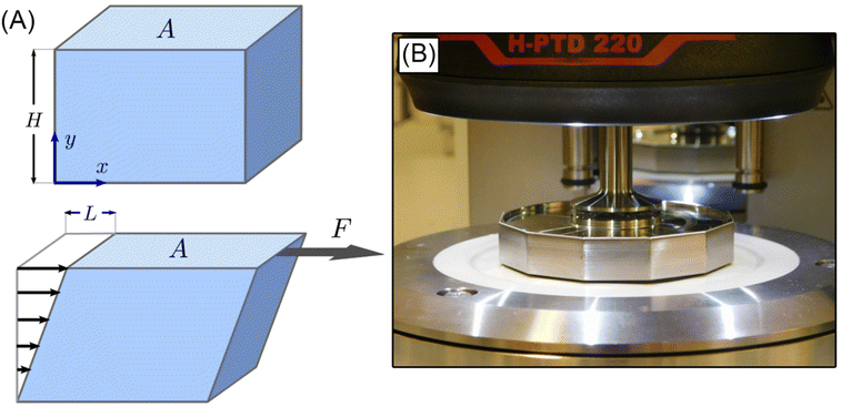Fig. 1 (A) Schematic of sample inside parallel plates geometry during a simple shear experiment. (B) Photograph of molten commercial polystyrene disc in a parallel plate rheometer.

The simple shear experiment may be described more formally by introducing the following terminology. The shear strain (γ, a unitless property) characterizes the magnitude of the applied deformation and is given by γ = L/H. Shear stress (σ, in units of pressure) is the magnitude of frictional force that travels down the y-axis divided by the interfacial area, i.e., σ = F/A. Typically, simple shear experiments involve a step strain, where γ is instantaneously ramped and maintained at a constant value. For the case where the top plate is continuously moved during the shear experiment, the strain rate (, in units of inverse time) is the rate of change of γ. It is equal to the velocity of the top layer divided by H, .

The movement of the top plate during simple shear deforms the sample, but the internal forces induced depend on the state of matter. For solids undergoing a minor deformation (i.e., γ ≪ 100%), σ follows Hooke's Law of elasticity which is denoted by the subscript “e”

σ_e = G₀γ (1)

where G₀ is the shear modulus that describes material stiffness. The shear modulus of metals and alloys is on the order of 10–100 GPa, while that of polymers and rubbers varies between 0.1–100 MPa, depending on the molecular details. The modulus of soft biological materials like muscle and tissues is on the order of 1–10 kPa.³⁴

Eqn (1) specifies a linear relationship between σ_e and γ. If a constant step strain is applied, as depicted in Fig. 2A, the corresponding σ_e also displays constant step behavior (Fig. 2B). If the step strain is removed, σ_e drops to zero instantaneously, and the solid returns to its original shape. The energy required to induce deformation is fully returned to the surroundings once the strain is released. This resistance against permanent deformation – a defining characteristic of a solid that is quantified by G₀ – is known as elasticity.

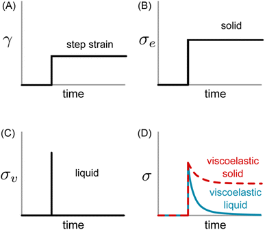Fig. 2 (A) Applied strain profile and resulting shear stress for (B) ideal elastic solid, (C) ideal viscous liquid, and (D) viscoelastic samples.

Liquids, on the other hand, obey Newton's Law

where the subscript “v” marks the response as viscous. The viscosity η₀, which is also referred to as the zero-shear viscosity by rheologists, characterizes the resistance to flow. It is a macroscopic manifestation of the internal frictional force between layers. At room temperature, the viscosity of water is 0.001 Pa s, while that of honey is 10 Pa s. The viscosity of bitumen, as measured by the famous pitch drop experiment, is on the order of 10⁷ Pa s.³⁵ Another unit of viscosity that is often encountered is Poise (1 Poise = 0.1 Pa s).

According to eqn (2), the σ_v of a liquid depends only on the rate of deformation, and not the magnitude of deformation itself. Consequently, during a simple shear experiment a liquid only experiences stress when the upper plate is moving. The resulting σ_v imposes a frictional drag force and drives the liquid to flow. When the upper plate stops moving, σ_v gradually falls to zero.

Thus, solids and liquids exhibit qualitatively different behavior in simple shear experiments. Elastic solids respond to the magnitude of deformation, while viscous liquids respond to the rate of deformation. As stated previously, solids store energy which can be fully recovered, while liquids dissipate energy which is lost to the surroundings as heat. These characteristics, however, are idealized and represent limiting behavior. Many condensed-phase materials do not readily fall into these classical categories because their mechanical properties depend on both the magnitude and rate of deformation. For example, consider toothpaste: it flows like a liquid, allowing it to be squeezed out of a tube, but maintains its shape like a solid once it is put on a toothbrush. Such materials are viscoelastic and are often called soft matter or complex fluids.^36,37

Fig. 2D outlines the simple shear behavior of two different types of viscoelastic materials. For both the viscoelastic solid and liquid, a step strain elicits an instantaneous elastic response which produces a spike in σ. Rather than remaining constant or immediately falling to zero, however, the stress decreases gradually. It approaches a finite plateau value for the viscoelastic solid at long times, while it decays completely to zero for the viscoelastic liquid.

This qualitative behavior is observed in all materials that have molecular or structural length scales much larger than atomic. Thus, virtually all polymers are viscoelastic. When they are subjected to a step strain deformation, the equilibrium conformation of individual chains is disturbed. At short time scales, the resistance of the chains against deformation materializes as a solid-like elastic response. As time progresses, the chains move and slide past one another to relax towards equilibrium, creating a liquid-like viscous response.

The chemical structure of the polymer plays a critical role in dictating the interplay between the elastic and viscous responses. Thermoplastics – in which the polymer chains exist as discrete molecules – fully dissipate stress because chains can diffuse freely when heated above the glass transition temperature. Molar mass, chain architecture, and backbone rigidity serve as the molecular knobs for tuning the diffusive and sub-diffusive motions. In contrast, thermosets contain polymer chains that are covalently bonded together by permanent cross-links. This architectural constraint prevents diffusion, so the chains cannot fully dissipate stress. For these reasons, thermoplastics are viscoelastic liquids while thermosets are viscoelastic solids.

CANs express rheological behavior closer to that of thermoplastics than thermosets. For instance, silly putty – a commercially available CAN of polydimethylsiloxane chains covalently cross-linked by dynamic boronate ester bonds –³⁸ flows at elevated temperature while permanently cross-linked polychloroprene does not (Fig. 3). At time scales shorter than the lifetime of the cross-link, CANs behave like viscoelastic solids. At longer time scales, they flow like viscoelastic liquids. In addition to polymer chain motions, however, CANs also dissipate energy through transient cross-linking. This additional energy dissipation mechanism provides another lever for controlling the polymer viscoelastic response.^22–26,39

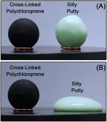Fig. 3 Spherical samples of permanently cross-linked polychloroprene (viscoelastic solid) and silly putty (viscoelastic liquid) during annealing at 50 °C. (A) t = 0 min and (B) t = 30 min.

The intimate relationship between polymer structure and viscoelasticity represents a direct path between the chemistry and material properties. For emerging materials like CANs, rheology plays a critical role in illuminating how structure governs viscoelasticity. Rheological experiments essentially probe the viscoelasticity of a sample by applying a strain and measuring a stress, or vice versa. There are many different types of rheological devices, but the simplest is the shear rheometer, which deforms a material by shearing it between a moving and a fixed solid surface – as was the case in the simple shear experiment described previously. Fig. 1B provides a photo of a shear rheometer measurement on commercial polystyrene. Due to the introductory nature of this tutorial review, we concentrate exclusively on linear rheology measurements of bulk polymers (i.e., no solvent), which are more readily described by molecular theories (see Box 2). Furthermore, we focus on shear rheology because, in the linear regime, all other linear rheological properties may be inferred from it.^32,33

Box 2 Linear versus nonlinear rheology

Rheological experiments can be classified as linear or nonlinear depending on the magnitude of the applied strain or stress. In linear rheology, the perturbations applied are gentle – theoretically infinitesimal – so that the equilibrium structure of the material remains undisturbed throughout the experiment. Practically, we use perturbations on the order of 1–10% to ensure that the material response is robust enough to measure. Since linear measurements are non-destructive, they are most useful for investigating basic relationships between molecular structure and viscoelasticity.

In nonlinear rheology, we apply moderate to large deformations/torques, stretching and severely distorting polymer chain conformations. The goal of such experiments is to understand or predict material behavior during processing where strong flows are encountered. Nonlinear rheology experiments essentially reveal how large strains cause polymers to deviate from equilibrium behavior. Compared to linear experiments, however, they are more difficult to perform and interpret.

The boundary between the linear and nonlinear regimes can be probed using methods discussed in section 1.1.4.4. Measurements in the linear regime have several advantages: (I) all materials obey the Boltzmann superposition principle (see section 1.1.4) which provides a solid theoretical basis for interpretation, (II) experiments are straightforward to perform on modern rheometers, (III) standard experimental protocols and analytical tools are relatively well-established, and (IV) tensile properties can be directly inferred from shear measurements and vice versa.

1.1.2 Maxwell model. The Maxwell model (MM) is a simple phenomenological model for linear viscoelasticity (LVE). It consists of a Hookean spring and a dashpot – a piston-cylinder device filled with a viscous fluid – connected in series as shown in Fig. 4A. The spring captures the solid-like or elastic response described by eqn (1), while the dashpot mimics the liquid-like or viscous response described by eqn (2).

Fig. 4 (A) A Maxwell element consists of a spring and dashpot in series. (B) Linear–linear and (C) log–log axes plots of the stress relaxation of a Maxwell element subjected to step strain. The gray lines mark the location t = τ where the stress falls to 1/e of its initial value, i.e., σ(t) = σ(0)/e.

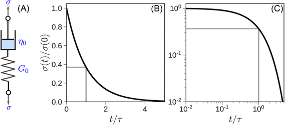
When an external tension or stress σ is imposed on the system, it induces an identical stress in each element – i.e., σ_e = σ_v = σ, where the subscripts “e” and “v” denote the elastic force produced in the spring and the viscous force produced in the dashpot, respectively. Meanwhile, the total extension or strain in the assembly is the sum of strain in each element, γ = γ_e + γ_v. Taking the derivative of γ with respect to time (denoted by the “dot” notation), we get

Substituting eqn (1) and (2) into eqn (3), we may write

It is useful to define a “relaxation time” τ = η₀/G₀ as the ratio of the viscosity and shear modulus. Then, the MM can be expressed succinctly as a linear differential equation

This is the constitutive equation for the MM that relates the evolution of stress in response to strain. For a step strain γ(t ≥ 0) = γ₀ applied at time zero, as illustrated in Fig. 2A, eqn (5) may be solved to obtain the stress profile

σ(t) = G₀γ₀e^−t/τ (6)

The response is shown graphically in Fig. 4B and C. Initially, the hypothetical material described by the MM stretches instantaneously and responds to the deformation like an elastic solid, σ(t = 0) = G₀γ₀, by storing the input energy in the spring. Subsequently, molecules wiggle around and gradually dissipate this stored energy, and stress relaxes exponentially. The stress relaxation modulus

G(t) = σ(t)/γ₀ = G₀e^−t/τ (7)

is a time-dependent modulus that is defined as the ratio of the time-dependent stress to the applied step strain. We observe that relaxation time τ controls the rate of stress relaxation and is formally equal to the time at which G(t) falls to 1/e of its initial value (i.e., 37% of G₀). Fig. 4C replots Fig. 4B on double logarithmic axes: this stretches out the curve at short times and squishes it at long times. As we shall see shortly, this is useful for polymeric materials whose G(t) is rich in features and can be measured over several decades of time.

While eqn (5) represents the differential form of the MM, it can be recast into an integral form using the method of integrating factors as

where the time t′ tracks the deformation history of the material up to the present time t. Eqn (8) shows how the stress at any instant is an integral of the relaxation modulus times the strain rate over the entire history of the material up to that instant. Due to the decaying exponential in the integrand, the MM has fading memory such that recent events matter more than those in the distant past.

1.1.3 Multimodal relaxation and relaxation spectrum. The relaxation modulus can be experimentally measured by performing a step strain experiment, as shown in Fig. 5A for a commercial polystyrene (PS, see Appendix: Experimental details of commercial polystyrene rheology measurements). As expected from the MM, G(t) decays with time. On closer examination, however, we find that the curve is stretched out, and any attempt to fit a single Maxwell element fails miserably. The dashed red curve in Fig. 5A shows one such failed attempt.

Fig. 5 Stress relaxation of commercial polystyrene (gray symbols) fit to (A) a single Maxwell element (dashed red line) and a superposition of 8 Maxwell elements (thick black line). Contributions of the individual modes to the overall response are shown by thin black lines. Schematic diagrams of multimode Maxwell (B) liquid and (C) solid. For (B), G(t) will eventually decay to zero. For (C), G(t) will plateau at G_∞. (D) The shapes of the discrete and continuous relaxation spectra extracted from the data in (A) using the program pyReSpect are similar. Terminal relaxation times based on different definitions (discussed in section 4.2) are indicated on the horizontal axis.

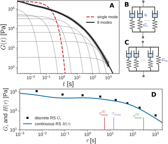
Instead of a single Maxwell element, we can consider a “multimode” MM in which several Maxwell elements are arranged in parallel, as shown schematically in Fig. 5B and C (see Box 3 for the multimode Voigt model, which uses a different arrangement of springs and dashpots). The G(t) of the multimode or generalized Maxwell model is given by a sum of decaying exponentials

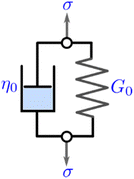
Box 3 Voigt model

The Voigt or Kelvin–Voigt model is a mechanical model for viscoelasticity that consists of the same fundamental elements as the MM, viz. a spring and dashpot.^47,48 Instead of being connected in series, however, the spring and dashpot are arranged in parallel as shown in Fig. 6.

Fig. 6 Schematic diagram of the Voigt model showing a spring and dashpot in parallel.

Thus, the strains in the spring and dashpot are identical, γ_e = γ_v = γ. The total stress is equal to the sum of the individual stresses . This leads to the differential equation

with τ = η₀/G₀. When such a system is subjected to a step stress σ₀ at time t = 0, it exhibits a classic retarded elastic response. This can be expressed in terms of creep compliance as

The MM is the simplest mechanical model for a viscoelastic liquid, and qualitatively describes stress relaxation in such materials. On the other hand, the Voigt model is the simplest rheological model for a viscoelastic solid and qualitatively describes creep and creep recovery in such materials. Yet, the “single mode” Voigt model described above, like the single mode MM illustrated in Fig. 4A, fails to capture quantitatively the viscoelasticity of real materials. In the generalized or multimode Voigt model, several Voigt elements are connected in series, often with an additional dashpot element to incorporate purely viscous behavior. Such generalized Voigt models may be used to quantitatively describe the LVE of both viscoelastic solids and liquids.

This raises the practical question: because the generalized Maxwell and Voigt models are flexible enough to simultaneously describe viscoelastic solids and liquids, which one should we use? Fortunately, the choice of which representation to use is a matter of convenience. In the literature, there appears to be a preference for the MM, which is also reflected in this tutorial review. In principle, any generalized Voigt model can be numerically mapped to an equivalent generalized Maxwell model and vice versa.^49,50

Here, G_∞ is the equilibrium modulus which is nonzero only for viscoelastic solids, such as polymer networks with permanent cross-links. For polymer solutions, melts, and transient networks with a sufficiently low degree of permanent cross-linking, G_∞ = 0. G_i, η_i, and τ_i = η_i/G_i represent the stiffness, viscosity, and relaxation times of the ith Maxwell element, respectively. In this review, we define the relaxation times so that τ₁ > τ₂ > … > τ_n. Thus, τ₁ is the longest relaxation time.

Each element in the multimode MM constitutes a “relaxation mode”. The set of relaxation modes {G_i,τ_i}ⁿ_i=1 is called the discrete relaxation spectrum (RS). In Fig. 5A, we find that using n = 8 relaxation modes allows the multimode MM to fit the commercial PS data quite well. The contribution of each of the 8 Maxwell modes is shown by a thin black line. It is also possible to define a continuous analogue of the discrete RS by replacing the summation in eqn (9) over the discrete modes by an integral. Thus, the continuous RS H(τ) is related to G(t) as

The discrete RS approximates the continuous RS; it has the same shape and general features (see Fig. 5D). Computer programs such as DISCRETE,⁴⁰ CONTIN,⁴¹ NLREG,⁴² IRIS,⁴³ or pyReSpect may be used to extract the continuous or discrete RS from experimental data.^44,45 The RS is of fundamental importance in LVE. It quantitatively describes the strength and speed of all the different relaxation mechanisms in a material. In principle, if the RS is completely characterized, then all LVE properties can be obtained mathematically from it. However, like the fable of the group of blind men and the elephant,⁴⁶ different experimental protocols measure different aspects of the RS. These protocols are described in the next section. Usually, it is important to piece together information from different tests to arrive at a holistic understanding of material behavior.

1.1.4 Standard linear rheology experiments. When a system at equilibrium is subjected to a tiny stimulus, it invokes a proportional response. In rheology, this regime corresponds to the LVE limit. Mathematically, the idea that small changes in strain produce proportionally small changes in stress can be expressed as dσ = Gdγ. It also can be written in terms of the strain rate as dσ = G(dγ/dt′)dt′. After substituting the time-dependent G(t) for the modulus to account for viscoelasticity, we can formally integrate the resulting expression to obtain the Boltzmann superposition integral or Boltzmann superposition principle (BSP)

The BSP is a general one-dimensional LVE constitutive model for all soft matter. All material-specific information is embedded in G(t). For example, we note that the multimode MM is a special case of eqn (11) with G(t) given by eqn (9). The BSP illustrates how the stress response to multiple independent perturbations (say ) is the sum of the individual responses to each stimulus.

The BSP is an extremely powerful tool for linear rheology. Once the RS or equivalently G(t) of a material is known, the BSP allows us to evaluate the stress response to any arbitrary deformation history. In theory, the only LVE test we need is a step strain or stress relaxation experiment. In practice, different experimental protocols are used because they are more convenient for a certain class of materials, or because they provide information over timescales of scientific interest.

Thus, the “holy trinity” of common linear rheological tests are stress relaxation, creep and recovery, and small-amplitude oscillatory shear (SAOS). These tests yield different LVE material functions. We have already seen how a step strain experiment yields G(t). Similarly, the creep test generates the creep compliance J(t). SAOS obtains the complex modulus G*(ω), a frequency-dependent material function. Table 1 summarizes the advantages and disadvantages of the different LVE experiments.

Table 1 Advantages and disadvantages of stress relaxation, creep and recovery, and small-amplitude oscillatory shear measurements

Experiment	Advantages	Disadvantages
Stress relaxation	Suitable for characterizing intermediate timescales	Signal gets weaker as time increases
	Relatively simple data analysis	Terminal relaxation is difficult to identify
Creep and recovery	Best for evaluating long time features in terminal relaxation regime	Tedious to confirm that tests are performed in LVE regime
	Terminal relaxation identified from steady-state flow regime	Creep ringing phenomena for highly elastic materials
	Signal gets stronger as time increases
Small-amplitude oscillatory shear	Best for probing dynamics at short timescales	Signal gets weaker as angular frequency decreases
	Resolves elastic and viscous contributions simultaneously	Low angular frequency measurements are time consuming
	Frequency and temperature sweeps may be performed
	Terminal relaxation identified from low angular frequency regime
	Avoids artifacts associated with step strain and stress experiments

---

1.1.4.1 Stress relaxation. The relaxation of stress σ(t) following a step strain γ₀ is the standard method for measuring the stress relaxation modulus G(t) = σ(t)/γ₀. The rheometer imposes γ₀ by rotating either the upper or lower plate to a specified angle. The resulting sample deformation creates a torque that is measured by a transducer. The measured torque is proportional to the shear stress and, consequently, G(t). In the LVE regime, increasing the magnitude of γ₀ proportionally increases the magnitude of σ(t), ensuring that the G(t) remains independent of γ₀.

Fig. 7 depicts experimentally measured G(t) profiles during stress relaxation of the commercial PS. For viscoelastic solids, such as a polymer network with many permanent covalent cross-links, G(t) approaches a finite plateau at long times – i.e., G(t → ∞) = G_∞. For viscoelastic liquids, G(t) decays to zero, as shown in Fig. 4C and 5A for a single mode Maxwell model and the commercial PS, respectively. The temperature dependence of viscoelastic properties is discussed later in sections 1.1.5 and 4.3. For now, we simply note that increasing the temperature results in faster relaxation.

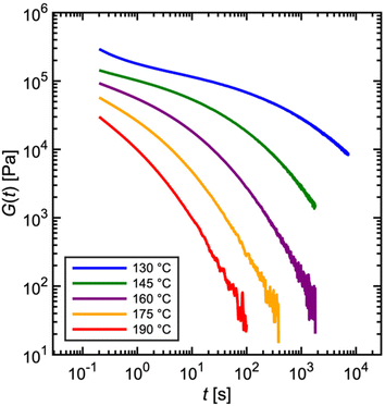Fig. 7 Commercial polystyrene stress relaxation at varying temperature. Stress relaxes faster as temperature is increased.

If the experiment is carried out for a time longer than the “terminal relaxation time” τ_term of the material, we observe the signature of “terminal relaxation”. As discussed in section 4.2, the precise definition of τ_term is context dependent, but the guiding principle is that at timescales larger than τ_term, the material effectively flows like a Newtonian liquid. In a stress relaxation experiment τ_term equals τ₁, the longest relaxation time in the RS. For t > τ_term, G(t) decays exponentially, i.e., ln G(t) ∝ t, and the constant of proportionality is equal to −1/τ_term. If a discrete RS is inferred from G(t) for such a material, then the zero-shear viscosity – defined as the area under the G(t) curve – can be obtained as

In practice, G(t) is rarely measured over more than three to four decades (see Fig. 7) in a single experiment for two reasons. (I) Imposed step strains are not instantaneous. Rather, rheometers approximate a step strain by ramping the strain sharply over a short time interval (see section 3.3). Due to the time required for stabilization, G(t) is only reliable for times greater than approximately 0.1 s, marking the lower end of the observation window. (II) If the experiment proceeds to very long times, stress eventually falls below the threshold of instrument sensitivity, setting the higher end of the observation window (see section 3.1). In general, rheometer transducers have difficulty in measuring a decaying stress over more than three orders of magnitude. For these reasons, step strain experiments are ideally suited for probing material relaxation over intermediate timescales between approximately 0.1 s at the lower end to 100–1000 s at the higher end.³³

Some readers might ask how then does the observation window for the relaxation modulus reported in Fig. 5A span over 6 decades? As described later in section 1.1.5, this involves a common “trick” to stitch together measurements at different temperatures – such as those shown in Fig. 7 – using a principle called time–temperature superposition.

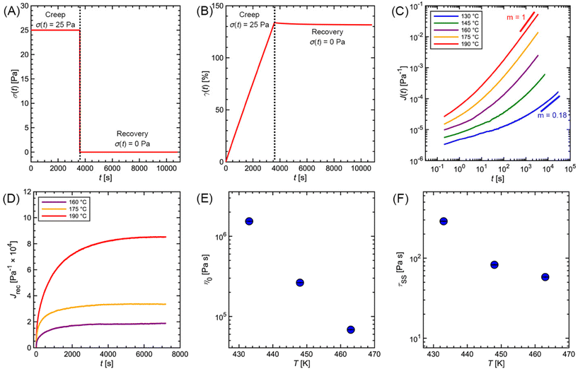
1.1.4.2 Creep and recovery. Creep and recovery tests make up a two-part measurement sequence that highlights long time viscoelastic behavior, making it ideally suited for studying terminal phenomena. In the first part (creep test), the rheometer applies a shear stress jump on the sample, rapidly ramping the stress from zero to an imposed value of σ₀. As the shear stress is held constant, the time-dependent deformation of the sample γ(t) is monitored. In the second part of the measurement (recovery test), the shear stress is released so that σ drops to zero. Consequently, the sample partially recovers its original shape, causing γ(t) to decrease over time.

Fig. 8A and B are the imposed σ and measured γ(t) profile during a creep and recovery test on commercial PS. During creep, the γ(t) of a viscoelastic liquid grows indefinitely as the sample can deform continuously without limit. The strain rate eventually becomes constant and exhibits “steady-state” behavior where γ(t) ∝ t. In contrast, for a viscoelastic solid, γ(t) reaches a plateau because the material cannot deform any further. During recovery, the magnitude of the γ(t) drop reflects the recoverable amount of elastic energy that was stored in the sample relative to the total amount of energy applied during the creep deformation.

Fig. 8 Commercial polystyrene creep and recovery measurement. (A) Applied stress and (B) measured strain profiles during creep and recovery. (C) Creep and (D) recoverable compliance versus time. (E) Zero-shear viscosity and (F) steady-state relaxation time versus temperature.

To normalize the material deformation response during creep, we can express γ(t) as creep compliance

J(t) = γ(t)/σ₀ (13)

Creep compliance has units of inverse modulus or 1/Pa. Yet, it is not simply equal to the reciprocal of the stress relaxation modulus, except at short and long times where J(0)G(0) = J(∞)G(∞) = 1. In the steady-state flow regime, where the creep compliance is linear with time, J(t) may be described by

where η₀ is the zero-shear viscosity and J⁰_e is the steady-state creep compliance. η₀, essentially a description of the liquid-like properties of the sample, is estimated from the slope of J(t) in the steady-state regime (Fig. 8C). J⁰_e, characterizing the solid-like traits, can be deduced from the intercept of the viscosity linear regression. However, this calculation is notoriously imprecise, as the J⁰_e extrapolation is highly sensitive to the bounds of the linear regression. While Ninomiya developed a method that reduces the uncertainty of the linear regression,⁵¹ estimation of J⁰_e from the creep test data alone is not recommended.

Rather, the recovery test permits more accurate determination of J⁰_e. The recoverable compliance J_rec is defined as

where t_f is the time at which the applied shear stress drops to zero, and γ(t_f) is the strain at the end of the creep test. As the sample recoils, J_rec increases towards a plateau value J^∞_rec (Fig. 8D). If – and only if – steady-state flow is reached in the preceding creep test, then the measured J^∞_rec= J⁰_e. Determining J⁰_e using recovery also improves the accuracy of η₀, as the linear regression of eqn (14) requires only a single fitting parameter. By performing both creep and recovery, a steady-state relaxation time τ_SS may be calculated by

τ_SS = J⁰_eη₀ (16)

Although the creep compliance and stress relaxation modulus are mathematically related by a convolution integral, J(t) is more convenient to study terminal behavior than G(t) for two reasons. (I) The signature of terminal relaxation may be clearly identified by the power law relationship between the creep compliance and time, i.e., J(t) ∼ t^m, where m is the power law scaling exponent. m corresponds to the slope of the long time region of the data in a log(J(t)) versus log(t) plot. If m ≈ 1, then steady-state flow has been achieved. Conversely, m ≪ 1 indicates the material has not reached terminal relaxation. (II) As the creep experiment proceeds, J(t) – and hence the signal from the rheometer – increases in magnitude for viscoelastic liquids, making it less susceptible to instrument sensitivity.

1.1.4.3 Small-amplitude oscillatory shear (SAOS). While stress relaxation and creep are transient experiments conducted over a fixed time range, small-amplitude oscillatory shear (SAOS) consists of several independent experiments conducted at varying frequencies. SAOS is arguably the most common rheological measurement for polymers because it concurrently resolves the elastic and viscous components of the material response. Unlike stress relaxation and creep, it achieves this without the need for making assumptions based on specific theoretical models. SAOS is best for studying short time phenomena.

Fig. 9 illustrates the imposed γ(t) and corresponding σ(t) profiles during SAOS. In this measurement, the rheometer applies a sinusoidal strain γ(t) = γ₀ sin(ωt) with amplitude γ₀ and angular frequency ω. Typically, γ₀ is held constant while ω is varied between 0.01 to 100 rad s⁻¹. The resulting σ(t) depends on the state of matter of the sample. For an elastic solid, eqn (1) predicts that the shear stress is linearly proportional to the applied strain. Consequently, the σ(t) during SAOS is perfectly in phase with γ(t), with its amplitude being equal to G₀γ₀. For a viscous liquid, eqn (2) states that the shear stress is proportional to the strain rate, i.e., the time derivative of the applied strain. The resulting σ(t) response is 90° out of phase with the applied γ(t), while its amplitude is equal to η₀ωγ₀.

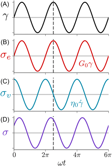Fig. 9 SAOS waveforms. (A) Applied strain, (B) solid, (C) liquid, and (D) viscoelastic measured shear stresses.

The SAOS response of a viscoelastic material lies between the elastic and viscous limits, with the phase angle between σ(t) and γ(t) being somewhere between 0 and 90°. The viscoelastic σ(t) profile can be uniquely decomposed into two parts: one that is in phase with γ(t), and the other that is in phase with the strain rate

σ(t) = γ₀[G′(ω)sin ωt + G′′(ω)cos ωt] (17)

G′ is called the elastic or storage modulus because its contribution to the total stress is proportional to the strain, like a Hookean spring. G′′ is called the viscous or loss modulus because its contribution to the total stress is proportional to the strain rate, like a Newtonian fluid.

It is common to define a complex shear modulus G*(ω) = G′(ω) + iG′′(ω) by combining the elastic and viscous moduli into a single term. The magnitude of G* is given by |G*(ω)| = ((G′)² + (G′′)²)^1/2, while the phase angle δ between σ(t) and γ(t) is given by tan δ = G′′/G′. For those familiar with electrical circuit design, this framework is identical to the dissipation factor equations for dielectric materials. G′, the real component of G*(ω), represents a solid-like contribution to the complex modulus. G′′, the imaginary component of G*(ω), depicts the liquid-like contribution. tan δ, colloquially known as the loss tangent or loss factor, quantifies the relative significance of G′ and G′′. tan δ ≪ 1 indicates the sample is more solid-like, while tan δ ≫ 1 signifies it is more liquid-like.

Mathematically, G*(ω) is related to the stress relaxation modulus via a modified Fourier transform

Using this relationship, the complex modulus corresponding to a generalized MM is shown to be

Fig. 10A illustrates the characteristic shapes of G′, G′′, and tan δ for a single mode MM. The angular frequency at which G′ and G′′ intersect, commonly referred to as the cross-over frequency ω_cross, demarcates the high and low frequency regions. Equivalently, ω_cross may be identified by tan δ = 1, and its inverse τ_cross = 1/ω_cross is sometimes used as a convenient proxy for τ_term (see section 4.2 for a more detailed discussion). In the high frequency region, G′ is constant because it reflects the behavior anticipated by Hooke's law. It is also much larger than G′′ due to the dominance of the elastic contributions towards G*. In contrast, the low frequency region represents terminal relaxation. G′′ is not only larger than G′, but it also decreases more slowly as ω decreases. Specifically, in the terminal relaxation regime G′ ∝ ω² and G′′ ∝ ω¹. If – and only if – these specific power law scalings are observed, then τ_term may be estimated by⁵²

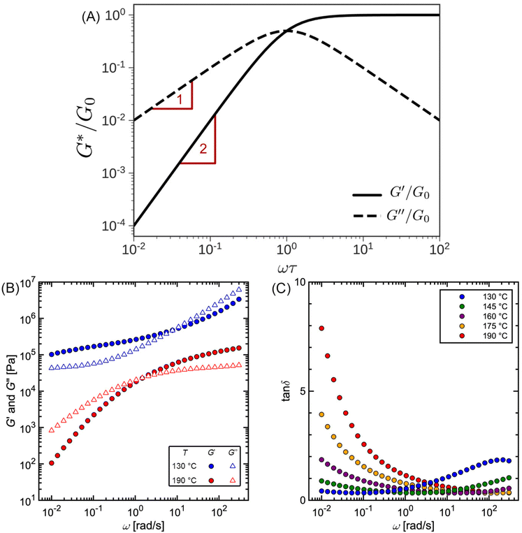Fig. 10 (A) SAOS moduli for single mode Maxwell model. (B) SAOS moduli and (C) tan δ for commercial polystyrene.

Fig. 10B and C depict experimentally measured SAOS data for commercial PS. While cross-over features are observed, the data look qualitatively different from the schematic portrayed in Fig. 10A. The additional features found in this data set are discussed in section 2.

As a complement to isothermal frequency sweeps, SAOS isofrequency temperature sweeps also may be conducted. This type of experiment tracks the evolution of G′, G′′, and tan δ as the sample is heated or cooled at a constant ramp rate, offering utility for detecting various thermal transitions. For example, the glass transition temperature corresponds to a large drop of several orders of magnitude in G′ and a peak in tan δ. The technique can also identify other types of thermal events, such as the melting of semi-crystalline polymers or the order–disorder transition of block copolymer nanostructures. Although temperature sweeps can be executed using a shear rheometer, they are commonly performed using specialized “dynamic mechanical analysis” instruments that utilize extension or torsion geometries. The success of these experiments hinges on the careful consideration of the ramp rate. If the ramp rate exceeds the rate of terminal relaxation – likely to be the case at low temperatures – the sample may deviate significantly from equilibrium behavior. To mitigate this, SAOS temperature sweeps are typically performed using ramp rates on the order of 1 °C min⁻¹ and a frequency of 1 Hz.³⁶

SAOS tests are practically useful for two main reasons. (I) Modern rheometers can perform frequency and temperature sweeps, and directly report the elastic and viscous moduli over a wide range of frequencies and temperatures. (II) SAOS avoids experimental and analytical challenges that arise from approximating step strains or stresses with sharp ramps (see section 3.3).

1.1.4.4 Finding the linear viscoelastic regime via SAOS and creep. The mathematical models for interpreting G(t), J(t), G′, and G′′ depend on the assumption that the elastic and viscous contributions to σ are linear with γ and , respectively. This relationship is true below some critical strain value (γ_crit), above which nonlinear effects become significant. To ensure that stress relaxation and SAOS measurements correspond to the LVE regime – i.e., the regime in which the modulus is independent of strain – γ_crit must first be determined.

Fig. 11A outlines a common protocol for identifying γ_crit involving strain amplitude sweeps. In this method, SAOS measurements are performed at a constant frequency (typically between 1 to 10 rad s⁻¹) and increasing strain amplitude γ₀ up to 100%. At low γ₀, G′ is essentially constant within noise limitations. As γ₀ reaches γ_crit, G′ begins to deviate greatly from its original plateau value. The commercial PS sample highlighted in Fig. 11A shows a steep decrease in G′, indicating damping behavior. Other types of samples, however, may exhibit more complicated nonlinear behavior.⁵³

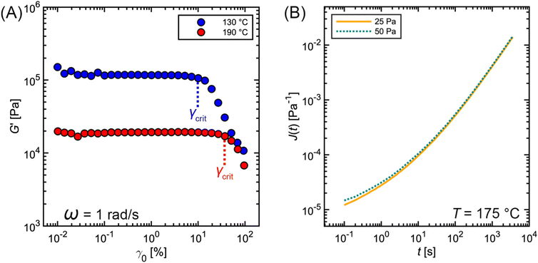Fig. 11 Commercial polystyrene (A) SAOS strain amplitude sweep and (B) creep measurements at varying shear stress.

Once γ_crit is identified, stress relaxation and SAOS experiments should be performed at γ₀ well below that value. While there is no strict guideline for identifying the optimal γ₀, a good rule of thumb is to use . This choice balances the tradeoff between noise which is visible at low γ₀ (see Fig. 11A) and nonlinear effects visible when γ₀ > γ_crit. γ_crit also has a thermal dependence, so it should be measured at temperatures that correspond to the upper and lower bound conditions of the planned experiments.

Determination of the LVE regime for creep is trickier (Fig. 11B) because it can only be performed retroactively. Essentially, creep experiments must be conducted at different σ₀, ideally differing by at least a factor of 2. If the measurements were performed in the LVE regime, then the creep data for the different σ₀ will collapse onto a single curve.^54–56 For softer materials, such as an unentangled polymer melt, σ₀ ≈ 10 Pa is commonly used. For harder materials, such as a highly cross-linked polymer melt, σ₀ on the order of 1000 Pa are employed.⁵⁷

1.1.5 Time–temperature superposition. As seen in section 1.1.4, LVE properties vary strongly with temperature. The primary effect of increasing temperature is a significant decrease in relaxation times. A secondary effect is a subtle change in modulus (or compliance). The modulus is proportional to the density and absolute temperature G ∝ ρ(T)T. As temperature increases, polymer density decreases due to thermal expansion, partially canceling the increase (T) due to entropic elasticity. This attenuation has also been observed in CANs.^38,92

An important empirical observation is that for many polymers the different relaxation times τ_i and moduli G_i that characterize the discrete RS exhibit the same functional dependence on temperature. This fortunate relationship means that a change in temperature results in a horizontal and vertical shift of G(t), J(t), G′, and G′′ on a log–log plot. The shapes of the LVE curves and the RS are preserved. Such materials, which allow for time–temperature shifting, are called thermorheologically simple. In the absence of phase transitions, temperature-dependent structural changes, or side reactions, most homopolymer melts and solutions are thermorheologically simple. For polymers, the microscopic origin of this phenomenon can be traced to segmental motions that set the fundamental clock for chain motion. If subchain motions rely only on this metronome, all relaxation processes inherit its temperature dependence.^22,58,59

Time–temperature shifting is enormously helpful in practical applications because it resolves the problem of limited time or frequency windows. We can measure LVE data at different temperatures and stitch them together through a process of alignment to produce a master curve that spans many decades. This technique, called time–temperature superposition (TTS), allows us to compress a large amount of experimental data and to express them using just the master curve and a plot of shift factors.^60,61

To illustrate how to apply this concept to experimental data, in the following paragraphs we guide the reader through the process using the commercial PS rheology data presented earlier in the tutorial. The supplementary spreadsheet “Supplementary Information_PS Rheology TTS.xlsx” contains the raw data and formulas needed to perform TTS. It is organized into four separate sheets containing data for shift factors, SAOS, stress relaxation, and creep. Instructions for using the spreadsheet are embedded within the shift factor sheet. The spreadsheet also may be used to perform TTS on other samples by replacing the data in the SAOS, stress relaxation, and creep sheets.

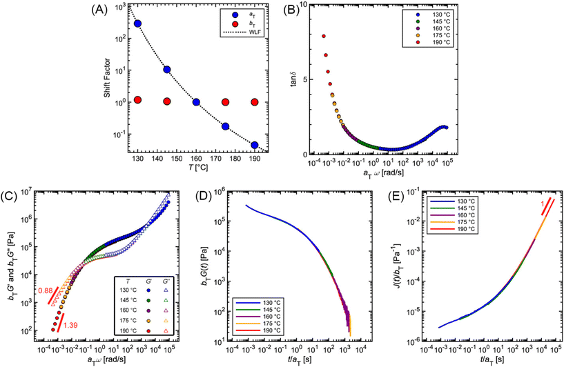
Fig. 12 and Table 2 depict the standard steps of the TTS process. First, we select a reference temperature T_ref, such that the data at T_ref will serve as a basis of comparison for the other curves. While any temperature could be used, we choose 160 °C because it is the middle temperature in our data set. Next, we estimate the horizontal (a_T) and vertical (b_T) shift factors required for superposition. By definition, a_T(T_ref) = b_T(T_ref) = 1. In terms of the MM, a_T – which shifts the curves left to right – describes the ratio of a τ_i at one temperature relative to the value at T_ref. b_T – which moves the curves up and down – accounts for corresponding changes in G_i.

Fig. 12 Commercial polystyrene time–temperature superposition using T_ref = 160 °C. (A) a_T and b_T shift factors. The WLF equation is fit to the experimental a_T values. (B) tan δ, (C) G′ and G′′ (D) G(t), and (E) J(t) master curves.

Table 2 Steps for applying time–temperature superposition

Step	Step description
1	Define a Tref
2	Take tan δ versus ω data. At each T, multiply ω by some value to shift data to form a continuous master curve. The value you use to shift ω is the aT for that temperature
3	Plot aTversus T. Compare aT to a model (e.g., WLF or Arrhenius) to refine values
4	Apply aT to G′ and G′′. If needed, shift curves vertically to estimate bT
5	Apply aT and bT to G(t) and J(t) to confirm validity

---

To systematically identify a_T, we recommend first aligning the tan δ versus ω curves because they are independent of b_T, so no vertical shifting is necessary (Fig. 12B). Keeping a_T(T_ref) = 1, the a_T values at other temperatures are varied until the data form one continuous master curve. Because a_T is proportional to relaxation time, it typically decreases by several orders of magnitude as temperature increases. This means that a_T > 1 for temperatures below T_ref, and a_T < 1 above T_ref. For the commercial PS SAOS data, application of a_T stretches the angular frequency range from approximately 10⁻⁴ to 10⁵, a span of 9 orders of magnitude (Fig. 12C).

After the initial estimate of a_T, the temperature dependence may be further refined by comparing the experimental shift factors to a model. A commonly employed empirical relation for polymers is the Williams–Landel–Ferry (WLF) equation

where C₁ and C₂ are model parameters that can be regressed from a plot of (T − T_ref)/log₁₀ a_Tversus T − T_ref. As seen in Fig. 12A, nonlinear regression creates great agreement between the experimentally determined a_T values and WLF equation. Close to the glass transition temperature, TTS generally fails for homopolymers due to fast relaxation modes that have a different temperature dependence. Far from the glass transition temperature (T ≫ T_g), the WLF equation takes an approximate Arrhenius formwith E_WLF = 2.303C₁C₂R. For some polymers, however, this behavior may be inaccessible due to thermal degradation.

After determining a_T, the values are then applied to G′ and G′′ to form master curves of the dynamic moduli. To improve the overlap, the G′ and G′′ data may be shifted vertically to estimate b_T. At each given temperature, the same b_T value is used to shift both G′ and G′′. For example, b_T values of 1.18 and 1.05 are applied for the 130 and 145 °C PS curves. At the other temperatures, b_T is kept equal to 1, demonstrating the relatively weak thermal dependence of the vertical shift factor.

As an additional validity check of the determined shift factors, TTS also may be performed on the stress relaxation and creep data. Using the same a_T and b_T values estimated from the SAOS data, master curves corresponding to G(t) and J(t) can be obtained by plotting b_TG(t) and J(t)/b_T, respectively, versus t/a_T. The superposition of the PS stress relaxation and creep master curves in Fig. 12D and E demonstrate excellent agreement with the SAOS data.

As seen from the PS example, TTS is a powerful tool for expanding the observation window of rheological data. Yet, care must be taken when applying the technique, as it relies on the critical assumption of thermorheological simplicity. While this is typically satisfied for linear homopolymers, it is not universally fulfilled by all macromolecular materials. For example, samples that undergo a phase transition or cross-linking are not thermorheologically simple. Neither are most polymer blends or block copolymers, as each component may have different temperature dependences. TTS also fails for polymers with large side groups or branching. Even for linear homopolymers, breakdown of TTS is observed at temperatures near T_g, where the motions of individual functional groups become important. In general, TTS only applies over some limited experimental range, and typically fails when the time and temperature windows are significantly broad. To quote Donald Plazek, winner of the 1995 Bingham medal awarded by the Society of Rheology: “the test for thermorheological simplicity can only be definitive in its failure: i.e., thermorheological complexity can be proven, simplicity cannot”.⁶²

2. Phenomenology of conventional polymers

The rich viscoelastic behavior of polymeric fluids originates from their macromolecular architecture. Nonlinear phenomena during processing – such as shear thinning, extensional thickening, and rod climbing – reflect the response of the chains after they are stretched and distorted by high strains and stresses. Even in the LVE regime, where the imposed deformation is minor, the observed rheological response of a polymeric material is tied intimately to its equilibrium chain conformation. In this section, we highlight commonly observed linear rheology features of conventional thermoplastic and thermoset homopolymers, thereby providing an initial framework for understanding the viscoelastic behavior of CANs.

Before proceeding, it is useful to clarify the terminology used to describe chain length. For the synthetic polymer chemist, chain length is typically quantified using the number average degree of polymerization, i.e., the molar mean of chemical repeat units within a polymer chain. In this context, the radius of gyration (R_g) is defined in terms of the number of repeat units, the length of bonds within each repeat unit, and a proportionality factor that accounts for the backbone stiffness. To avoid dealing with the details of local stiffness constraints, polymer physicists and rheologists commonly describe chain length in terms of an equivalent freely-jointed chain with an effective degree of polymerization N. Under this framework, R_g relates to N by the expression

where b is the statistical segment length or the “Kuhn” segment length. A statistical segment accounts for backbone stiffness and typically subsumes several chemical repeat units. It does not have a direct relationship to the monomer size or chemical structure. To be consistent with the macromolecular rheology literature, the following discussion uses the effective degree of polymerization N to describe molar mass effects on polymer viscoelasticity.^22,58,59

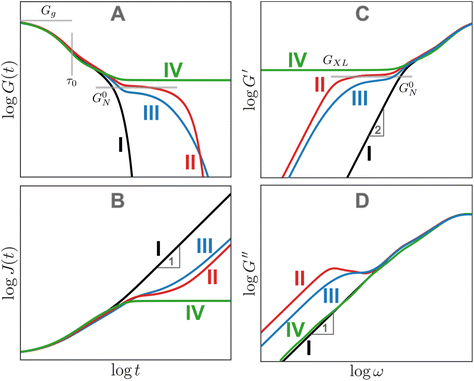
Fig. 13A shows the typical G(t) for various homopolymer systems that differ in molar mass distribution and topology but share the same repeat unit chemistry. The short time plateau in G(t) is called the glassy modulus; its magnitude is symbolized by G_g. For polymers, G_g is on the order of 1 GPa. After the glassy plateau regime, the modulus begins to decay due to relaxations of individual repeat units and chain segments. These rearrangements, commonly referred to as segmental motions, are largely controlled by the vibration of atomic bonds and bond angles at the level of a monomer. Because these dynamics correspond to length scales commensurate with the individual repeat unit, viscoelastic behavior in this regime is independent of N. The subsequent shape of the relaxation modulus, however, arises from the rearrangement of polymer strands at various length scales.

Fig. 13 Schematic for the (A) stress relaxation modulus, (B) creep compliance, (C) storage and (D) loss moduli of typical polymeric systems: (I) unentangled melt, (II) entangled melt, (III) polydisperse melt, and (IV) permanently cross-linked rubber.

Curve I depicts a monodisperse linear polymer melt with relatively low molar mass. The onset of relaxations at length scales corresponding to a statistical segment is marked by τ₀. Immediately after τ₀, the relaxation modulus exhibits an apparent power law scaling G(t) ∝ t^−½. These dynamics are captured by the Rouse model, which visualizes polymers as a set of Brownian particles connected by springs. The power law regime represents coordinated motions of chain segments shorter than N. Eventually, the G(t) curve decays exponentially at times greater than the terminal relaxation or Rouse time τ_Rouse. For linear polymers, τ_Rouse also represents the average time it takes an individual chain to diffuse a distance equal to its R_g.^22,58,59

The viscoelastic response of the Rouse model may be described by

τ_Rouse = τ₀N² (27)

where ρ is density, R is the gas constant, T is temperature, and M₀ is the molar mass of the statistical segment. Comparison of eqn (25) to (9) demonstrates that the Rouse model is basically a multimode Maxwell model in which τ_i = τ_Rouse/i².

Curve II corresponds to a monodisperse polymer chain with relatively large molar mass. When the chain length is larger than some critical value, a secondary plateau appears between the segmental motion and terminal relaxation regimes. This feature, commonly called the rubbery plateau, is caused by entanglements – essentially knots that form between long chains. The entanglement phenomenon is purely physical in origin and is related to how long cables or spaghetti tangle spontaneously. Entanglements can be thought to be temporary cross-links with special properties. Unlike temporary crosslinks in CANs, entanglements constrain only the lateral displacement of chain segments, while permitting chains to slide along their contours. Consequently, entanglements are released as individual chains slide past each other. Eventually, they disentangle (and re-entangle) via a process called “reptation”, allowing the polymer to diffuse and relax the remaining stress. Entanglements dominate the viscoelastic behavior once the number of statistical segments exceeds the entanglement value of N_e. Typically, the rubbery plateau appears once the number average number of entanglements per chain (N/N_e) exceeds a ratio of 2 to 5. The magnitude of the rubbery plateau modulus (G⁰_N) is on the order of 1 MPa, and is proportional to the spatial density of entanglements through the relationship

While G⁰_N is a function of N_e, it does not depend on the total chain length or N/N_e. In contrast, τ_term varies quite strongly with chain length, showing a power law dependence of τ_term ∝ (N/N_e)^3.4 for many real polymers. N_e for a particular polymer chemistry may be found in a database or estimated from measured G⁰_N values.^22,58,59

While curves I and II describe polymers with low molar mass dispersity, curve III depicts a polymer with high molar mass dispersity. This behavior is representative of most commercial polymers, which often contain a mixture of unentangled and entangled polymer chains of different chain lengths. For high dispersity samples, a diffuse rubbery plateau appears when the weight average N is significantly larger than N_e. Consequently, the rubbery plateau may be reduced to a shoulder, and its G⁰_N may be lower than monodisperse entangled melts with the same N due to the dilution effect of short chains. Furthermore, terminal relaxation can be stretched out by a small fraction of exceptionally long chains in the mixture.

Finally, curve IV shows the expected behavior of a polymer with a high number of permanent covalent cross-links. While segmental motions of the network strands dissipate some stress, long range motion and chain diffusion are ultimately stymied by the cross-links, causing the material to behave as an elastic solid at longer times. Similar to entangled polymers, cross-linked polymers exhibit a plateau regime. The magnitude of this plateau (G_XL) is proportional to the density of cross-links rather than entanglements

where N_XL is the average number of cross-links per chain. Thus, increasing the cross-link density creates a material with greater rigidity.

The G(t) of entangled polymers with temporary crosslinks can show two plateaus, where both entanglements and crosslinks contribute to the higher plateau. To a first approximation, the stress relaxation of CAN materials resembles curve II for entangled polymers because the effects of entanglements and dynamic covalent cross-links are qualitatively similar.

While Fig. 13A focuses on G(t), Fig. 13B–D illustrate the analogous J(t), G′, and G′′ curves. For J(t), the unentangled polymer melt (curve I) and the cross-linked polymer (curve IV) mark the two extremes. J(t) eventually becomes proportional to t for viscoelastic liquids (curves I–III). It approaches a permanent plateau for the crosslinked polymer with a height given by the inverse of the cross-link plateau modulus 1/G_XL. The J(t) for the entangled polymer melts shows a shoulder before approaching steady-state flow. As a first approximation, G′ curves appear to be reflections of the corresponding G(t) curves. Plateaus corresponding to entanglements and cross-links are observed in the G′ curves for all cases except the unentangled melt. No plateaus are evident in the G′′ curves. However, local maxima in the G′′ curves mark the location of sharply defined relaxation processes, such as the terminal relaxation regime observed in curves II and III. Box 4 provides more context regarding long and short timescales.

Box 4 Long and short timescales

At several points in this tutorial review, the labels “long” and “short” timescales are used without explicitly specifying a point of comparison. In general, long timescales refer to an observation timescale τ_obs that is much longer than the terminal relaxation time where the entire system has had a chance to relax, i.e., τ_obs ≫ τ_term. On the other hand, short timescales refer to τ_obs ≪ τ_term, when relaxation is confined to only a few segments. Viscoelastic liquids such as CANs are solid-like at short timescales, and liquid-like at long timescales, as seen vividly for silly putty in Fig. 2. This allows silly putty to bounce elastically since its τ_term ∼ 0.1 s is longer than the typical timescales that correspond to impact, τ_obs ∼ 0.1–10 ms.^63,64

The distinction between long and short timescales has important practical consequences for designing materials with desired properties for specific applications. Typically, τ_obs is determined by the application of interest, and the goal is to control τ_term to elicit the appropriate viscoelastic behavior. Webber and Tibbitt suggest a useful framework for designing dynamic polymer networks. For injection and spraying applications, τ_term < τ_obs so that the material can be easily squeezed out of nozzles. For printing and molding applications, τ_term ≈ τ_obs to enhance processability and self-healing through bond exchange. For reprocessable plastics, τ_term ≫ τ_obs under ambient conditions so that they do not fail during use.⁶⁵ In many of these operations, temperature can be used as a knob to control τ_term. For example, during printing, recycling, or injection applications, the material may be heated to temporarily lower its τ_term, thereby promoting flow.

Viscoelastic properties of certain foods may be optimized by controlling τ_term to ensure a desirable texture. The timescales associated with chewing and swallowing are τ_obs ∼ 10–100 ms.³⁴ If τ_term ≫ τ_obs, the material may be too elastic and cause problems with swallowing and mouthfeel. In a similar vein, controlling the ratio of viscous and elastic contributions (by controlling τ_term and tan δ) at operating conditions is important for many applications, such as the design of rubber mats to dampen vibrations of industrial equipment. The viscous contribution must be large enough to absorb and dissipate mechanical vibrations.^64,66,67 Analogous considerations also apply in the design of viscoelastic noise-reduction materials which must be able to absorb and dissipate mechanical oscillations due to acoustic waves in the audible frequency range. Interestingly, the incorporation of rubber crumbs recycled from waste tires into asphalt mixtures not only improves the durability of pavements, but also decreases vehicular noise pollution.⁶⁸

3. Sources of experimental artifacts

While rheometers are very complex instruments, their function is simple: they apply a displacement and measure mechanical load (like force and torque) or impose a load and monitor displacement. Strain-controlled rheometers use the first approach, employing a motor to set the displacement while a separate transducer measures the resulting stress. Stress-controlled rheometers use the second approach, integrating the motor and transducer into a single unit. Generally, stress-controlled rheometers tend to be less expensive compared to their strain-controlled counterparts. Both types of rheometers are well-suited for linear viscoelastic measurements, as the material functions for stress relaxation, creep, and SAOS may be interconverted in this regime. For non-linear measurements, however, the control mode plays a critical role.^32–34

For both rheometer types, the measured displacement and torque signals are converted into an electrical current or voltage. Computer software then translates the electrical signals into viscoelastic properties such as modulus and compliance. Although the models used to calculate these properties are material-agnostic, they rely on several simplifying assumptions. Violation of these assumptions causes inaccurate determination of modulus and compliance, produces experimental artifacts in the data, and risks misinterpretation of viscoelastic behavior. This is especially concerning for CANs, as their viscoelastic behavior remains a field of study with many unresolved questions. As summarized in Table 3, the following sections identify common rheological artifacts produced by non-ideal experimental conditions. Box 5 discusses the properties of various shear rheometer measuring geometries.

Table 3 Types of experimental rheology artifacts

Artifact type	Impact on measurement	Mitigation strategy
Minimum torque	Noisy G(t), G′, and G′′ data	Increase γ0 and decrease Kτ
Thermal degradation	G′ and G′′ at constant frequency change over time	Identify upper temperature bound using thermal stability measurements
Instrument inertia	G′ ∝ G′′ ∝ ω^2 at high angular frequencies	Lower ω in SAOS measurements
	G(t) and J(t) display oscillations at short times	Reduce sample thickness in stress relaxation and creep
	J rec parasitic drift at long times	Apply linear regression on Jrec to remove parasitic drift
Underfilling/overfilling	Creates inaccurate estimate of moduli and compliance values	Impose a constant normal force
Slip	G(t), J(t), G′, and G′′change as a function of sample thickness	Impose a constant normal force
		Use plate geometries with roughened surfaces
		Glue sample to plate geometries

---

Box 5 Measuring geometries

Shear rheometers play a pivotal role in the investigation of polymer materials, spanning from low viscosity solutions to highly entangled melts. Their versatility stems from their capacity to employ different types of measurement geometries. For polymeric samples, the three prevailing geometries are parallel plates, cone and plate, and concentric cylinders.

The parallel plates geometry, the most common choice for bulk polymer and CAN melts, sandwiches samples between two circular flat disks (see Fig. 1B). Plates with diameters of 8, 25, and 40 mm are commonly used. The use of parallel plates permits facile sample loading and adjustment of gap height, rendering it the preferred geometry for highly viscous samples. Its main drawback, however, is that it does not apply a uniform deformation. Rather, the sample strain varies with the radius, so that the edges of the sample experience a larger strain than the interior. Consequently, the stress measured by the rheometer is a spatial average of the actual stress experienced by the sample. Caution is paramount when employing parallel plates for heterogeneous samples, such as phase-separated blends or nanocomposites, as the varying strain field may cause non-linear behavior to manifest in different regions of the sample.

The cone and plate geometry, on the other hand, achieves uniform strain. This setup compresses the sample between a flat bottom plate and a conical top plate with a truncated tip. The angle of the cone, which ranges from 0.5 to 4°, ensures the application of an even shear field throughout the entire sample. For this reason, it is the preferred choice for non-linear shear rheology measurements, as it simplifies the data analysis. It also is useful for studying heterogeneous samples. The cone and plate geometry, however, requires a fixed measuring gap between 30 to 150 μm. When dealing with colloidal samples, it is crucial to ensure that the particle sizes are at least one order of magnitude smaller than the gap height to avert the potential risk of jamming at the conical top plate tip. The narrow gap also complicates the loading of highly viscous samples.

The concentric cylinders geometry – also referred to as the Couette geometry, named after the French physicist Maurice Couette – is frequently used for systems with viscosities lower than 100 Pa s. The sample is confined to a narrow gap between an inner cylindrical bob and an outer cylindrical cup. The key advantage of this geometry lies in the substantial contact area between cylinders. For low viscosity fluids that produce minimal stress upon shearing, increasing the radii, length, or gap distance of the cylinders amplifies the torque. While most of the stress stems from the gap between the cylinders, the stress contribution of the fluid at the bottom of the cup also must be considered. As with the cone and plate, the concentric cylinders geometry requires great care to make sure that any particles within the sample are much smaller than the gap between the cylinders. An excessively large gap, however, may lead to the development of secondary flows that compromise stress measurements. Additionally, particle sedimentation at the bottom of the cup may occur for highly concentrated colloidal samples.^32,33

3.1 Minimum torque

The minimum torque detectable by a rheometer (T_min) depends on the type of instrument and sample geometry that are used. Commonly, a nominal T_min is reported in the Technical Specifications Data Sheet of a rheometer. For example, the Anton Paar MCR 302e and TA Instruments HR 30 both have reported T_min values of 1 nNm for constant shear measurements. For oscillation measurements, T_min drops to 0.5 and 0.3 nNm, respectively.^69,70 While these values are specified by the rheometer manufacturers, in practice T_min is also affected by contributions from surface tension and inertial effects.⁷¹ As a conservative estimate, only torque values two to five times larger than the nominal T_min should be trusted. Fig. 14A applies these limits to the commercial PS stress relaxation data.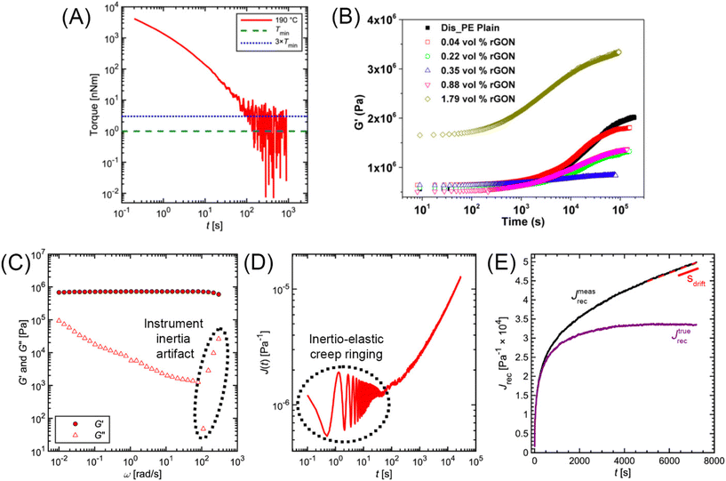

Fig. 14 (A) Minimum torque limits applied to commercial PS stress relaxation data at 190 °C. Data were collected using an Anton Paar MCR 302e rheometer. 3 × T_min was used as the torque cut-off. (B) Time sweep measurements to evaluate thermal degradation of polyethylene containing reduced graphene oxide. Adapted from ref. 73. Copyright 2015 American Chemical Society. (C) G′′ instrument inertia artifact observed at ω ≥ 100 rad s⁻¹. (D) Inertio-elastic creep ringing observed in the J(t) of a polybutadiene vitrimer at 160 °C. (C) and (D) Adapted from ref. 92. Copyright 2023 American Chemical Society. (E) Calculation of J^true_rec for commercial PS at 175 °C.

For stress relaxation and SAOS measurements, a minimum detectable modulus (G_min) may be estimated using the relationship

where γ₀ is the applied strain and K_τ is a constant that depends on the sample geometry. For a parallel plates configuration, where R is the plate radius. The measured G(t), G′, and G′′ must be larger than G_min for the data to be reliable.^33,71

For SAOS, low torque also leads to artifacts in the measured elastic modulus G′ of samples undergoing terminal relaxation. Specifically, the G′ uncertainty is expressed as , where is the phase angle. Within the terminal relaxation regime, decreasing ω not only amplifies the term due to diminished torque values, but also results in a substantial increase in tan δ dδ due to δ → 90°. Furthermore, at low torque the measured value of δ deviates greatly from its true value (greater than 5%).²⁷ The confluence of these errors can cause the measured G′ to deviate from the expected G′ ∝ ω² terminal relaxation scaling relationship, as seen in Fig. 2A in ref. 27.

Eqn (30) points towards strategies to improve the quality of stress relaxation and SAOS data via reducing G_min. For parallel plates, using a larger plate radius, larger γ₀, or both will decrease G_min. However, γ₀ must be less than γ_crit, as determined from strain amplitude sweeps, to ensure experiments are performed in the LVE regime.

3.2 Thermal degradation

For high T_g and well-entangled polymeric systems, significant relaxation may be only observed at temperatures well above 100 °C. Because most polymeric materials are organic, however, they are prone to oxidative degradation at these conditions. The molar mass of polydienes may increase due to radical-induced branching and cross-linking, leading to an increased plateau modulus. Poly(methyl methacrylate), in contrast, may depolymerize if its bulk ceiling temperature of 200 °C is surpassed.⁵⁹ Oxidation also causes polymer samples to discolor into a dark shade of brown, thereby ruining the optical properties. Furthermore, many CAN systems are susceptible to deterioration and side reactions when exposed to elevated temperatures for extended periods of time.^17,18 While thermal degradation may be impossible to fully inhibit, especially for very long experiments, its effects may be minimized to ensure that the measured data are representative of the original sample.

In addition to basic thermal characterization (e.g., thermal gravimetric analysis and differential scanning calorimetry), sample stability may be investigated using constant frequency time sweep SAOS measurements. Under this protocol, for a given angular frequency the evolution of G′ and G′′ are tracked over time to determine the extent of degradation. Increasing moduli suggest the sample is undergoing cross-linking, while the reverse insinuates depolymerization.⁷²

The main strategy for reducing thermal degradation is to perform the rheology measurements under an inert atmosphere. In this case, the sample geometry is encased in a hood that is flooded with nitrogen or argon gas. Increasing gas flowrate decreases the rate of degradation. Peltier hoods generally require much lower flowrates than convection ovens due to their difference in size, an especially important consideration for rheometers in which the inert gas is sourced from an individual cylinder rather than a shared storage tank. For systems involving solvent, however, flowing inert gas will induce evaporation.⁷²

A complementary strategy is to lace the sample with a stabilizing additive. Several types of antioxidants are commonly used for rubbers and styrenics. Polymeric epoxy and carbodiimides are effective for polyesters. Recent studies even suggest that reduced graphene oxide acts as an effective stabilizer (Fig. 14B). Trace amounts (≈0.1 wt%) are sufficient to minimize degradation.^73–75

3.3 Instrument inertia

Stress-controlled rheometers combine the motor and transducer onto a single shaft, thereby reducing cost and simplifying temperature control. While practical, this combination is prone to inertial effects because acceleration of the motor creates additional torque that is detected by the transducer. The transducer itself also has inertia that contributes to the torque signal. Although rheometer software accounts for some of these contributions, instrument inertia creates artifacts that may look like real data, thereby misrepresenting the sample response at very short time scales.

Instrument inertia creates several types of artifacts in linear rheology measurements. In SAOS, for example, it causes δ to be inaccurate at higher ω values. This is particularly problematic in scenarios where high ω coincides with tan δ → 0, such as within the rubbery plateau regime of entangled polymer and CAN melts. Because the measurement error of the viscous modulus is described by , the inaccuracy in δ creates sharp drops and upturns in the G′′ curves (Fig. 14C).²⁷ For low viscosity polymer melts and solutions, the increasing contribution of inertia causes G′ ∝ G′′ ∝ ω² and δ > 90°. Although inertial contributions can be subtracted from the total torque signal, this calculation becomes inaccurate at higher frequencies where inertia dominates the overall signal.⁷¹ For stress relaxation and creep measurements, inertia greatly impacts the quality of the data. The signal produced in response to a step strain or stress is not monotonic but is instead an oscillation that dampens over time (Fig. 14C). These oscillations – often referred to as inertio-elastic creep ringing – dampen more quickly if the sample thickness is reduced.⁷⁶ While this sinusoidal signal is generally considered a nuisance and is discarded, it does contain actual information about the sample viscoelasticity. Specifically, G′ and G′′ may be estimated for frequencies higher than those accessible by SAOS. The data analysis for this type of calculation, however, is non-trivial.⁷⁷

To alleviate the influence of inertia on stress relaxation and creep measurements, one viable approach is to decrease the thickness of the sample. An excessively thin sample, however, introduces additional complications, particularly for high modulus samples. In such cases, the rotational stiffness of the rheometer – i.e., the motor and measuring geometry – may become comparable to that of the sample, thereby corrupting the measured material properties.²⁸

Instrument inertia appears in creep recovery data as parasitic drift (Fig. 14D). Although the nominal shear stress during recovery should be zero, the air bearing that supports the rheometer drive shaft may retain some residual torque during the cessation of flow. As a result, J_rec does not reach a steady-state plateau, but instead exhibits a steady-state linear relationship with constant slope (i.e., parasitic drift). The magnitude and direction of the residual torque varies for each measurement. Fortunately, the residual torque artifact may be removed from the data using the following equation

where J^true_rec is the true recovery compliance of the sample, J^meas_rec is the measured recovery compliance, t_f is the time point in which the shear stress was removed, and s_drift is the slope of the parasitic drift portion of J^meas_rec.⁵⁶

3.4 Underfilling/overfilling

Modeling of a shear rheology experiment in a parallel plates geometry assumes that the edges of the sample are cylindrical and flush with the edges of the plates.³³ Underfilling of a sample between the plates will severely decrease the measured torque, leading to underestimated modulus and compliance values. The presence of an air/sample/plate interface creates surface tension forces that affect the torque. Overfilling the gap also will compromise the torque signal.⁷¹

Maintaining proper sample volume is especially challenging for experiments that span a wide temperature range due to thermal expansion or contraction of the sample. For example, Fig. 15A and B show a commercial polyisoprene sample that greatly contracts as it is cooled from 60 to −40 °C, leading to significant underfilling in the parallel plates geometry. To mitigate this issue, modern rheometers may be programmed to impose a normal force – i.e., a mechanical load perpendicular to the top face of the sample. As the sample changes temperature, the rheometer alters the sample height to maintain the prescribed normal force, thereby keeping the volume between the plates filled with material. For soft materials, a normal force ≈0 is sufficient. For stiffer materials, normal forces of approximately 1 N or greater may be needed. Too large of an applied normal force, however, can damage the rheometer.⁷⁸ For long experiments, relying solely on the normal force strategy may prove unsatisfactory, primarily because the gap height may evolve continuously throughout the measurement duration. The rheometer software may not accurately track the variations in strain resulting from the evolving gap, thereby introducing errors in the measured stress.²⁸

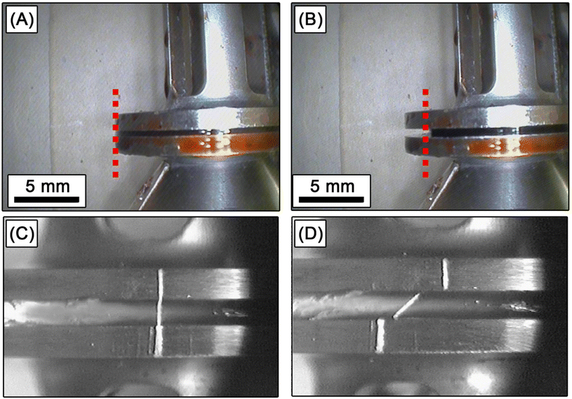Fig. 15 (A) and (B): Thermal contraction of commercial polyisoprene in a 25 mm parallel plates geometry. Red dashed line marks the outer edge of sample. (A) At 60 °C, sample is perfectly flush with edges of plates. (B) When cooled to −40 °C, sample volume significantly contracts. (C) and (D): Straight marker line test to identify wall slip during an applied step strain on molten polyethylene at 190 °C. 25 mm parallel plates geometry was used. (C) Before and (D) after step strain is applied. Adapted from ref. 79. Copyright 2001 American Institute of Physics.

3.5 Slip

Slip occurs when the sample interface and plate boundary have different velocities (Fig. 15C and D). In contrast to viscous liquids, polymer melts exhibit slip when the shear stress at the plate boundary exceeds a critical value σ_slip. Consequently, the actual strain experienced by the sample is smaller than the targeted value. The risk of slip is critical to consider for stress relaxation experiments due to the relatively high strain rate imposed when a step strain is applied.^79–81 Experimental investigations demonstrated that slip becomes more severe as polymer molar mass increases.⁸²

The main signifiers of slip are apparent stress and strain rates that change based on the geometry gap H. When slip occurs, it produces a gap independent contribution to the overall sample interface velocity v_top, thereby increasing the magnitude of the applied strain rate . Consequently, decreasing the geometry gap decreases the apparent stress.⁷¹

The contribution of slip may be minimized through careful experiment design strategies. Repeated measurements at varying H may be used to extrapolate the true stress value. Alternatively, adhesion between the sample and solid boundaries may be improved by using sandpaper or profiled plates. Application of a normal force also may minimize slip. As an extreme measure, the sample may be glued to the plate using adhesive. However, great care must be taken to ensure that the viscoelastic response of the glue does not affect the measured rheological signal.⁷¹

4. Best practices for covalent adaptable networks

Covalent adaptable networks (CANs) contain linkages between polymer chains that reversibly exchange by a chemical reaction, allowing the network topology to re-arrange. Cross-link exchange may proceed through either a dissociative or associative mechanism (Scheme 1). In the dissociative case, the two moieties connected at a cross-link junction (A and B) react with a neighboring functional group (C). B can switch places with C, leading to an overall change in topology. When this exchange occurs, the bond between A and B is first eliminated, leading to a reduction in the network connectivity during the reactive intermediate state. In the associative case, C connects to the cross-link junction before the bond between A and B is eliminated. Consequently, de-cross-linking does not occur because network connectivity is maintained.^17,18

Scheme 1 Mechanisms of cross-link exchange in CANs: (A) dissociative and (B) associative.

The difference in the cross-link exchange mechanism has significant impact on the viscoelastic behavior. When a dissociative CAN is heated, the loss of network connectivity causes a drastic reduction in G_XL. Eventually, it passes through a sol–gel transition to form a liquid. In contrast, an associative CAN does not exhibit a sol–gel transition due to its cross-link density being constant. Because the first generation of associative CANs exhibited rheological behavior similar to that of vitreous silica, associative CANs are more commonly referred to as vitrimers.^17,18

As rheology provides a framework for connecting the observable viscoelastic behavior of a material to its underlying chemical structure and morphology, it serves as the predominant tool for evaluating the impact of CAN molecular structure. The most practiced rheological approach demonstrated in the CAN literature is the use of stress relaxation measurements at varying temperature. Relaxation times are estimated by applying the single mode Maxwell model. While this strategy is common due to its convenience, it is flawed because it invokes an a priori assumption about the thermorheological behavior. Furthermore, the quality of stress relaxation degrades at longer times as the signal approaches the minimum torque limit of the rheometer. Because these issues create a severe risk of data misinterpretation and incorrect molecular understanding, stress relaxation measurements alone are not sufficient for accurately characterizing CAN viscoelasticity.

Fortunately, rheology offers great utility beyond stress relaxation measurements. Relaxation times may be determined directly from the data without the use of any restricting assumptions. As a complement to stress relaxation, SAOS and creep measurements offer deeper insight into the dynamics at short and long times, respectively. In the following sections, we highlight best practices for designing experiments and interpreting data for investigating CAN viscoelasticity.

4.1 Proper plotting of rheology data

CANs are complex materials comprising long chain molecules and transient covalent cross-links. Dynamics of the backbone and cross-links occur over widely separated time scales, and exhibit different temperature dependences. To resolve the viscoelastic fingerprints of CAN relaxation, rheological data must be plotted in a format that correctly represents the dynamics over a wide temporal range.

Fig. 16 illustrates the importance of correct plotting by graphing stress relaxation data of a polybutadiene vitrimer with dioxaborolane cross-links. Both panels A and B depict the same data sets at temperatures of 80 and 160 °C. Panel A, however, plots the data using a linear axis for modulus and a logarithmic axis for time. The modulus is also normalized by the value at t = 0.1 s, i.e., G(t = 0.1 s), the first recorded data point at each temperature. The dashed horizontal line indicates when the normalized moduli decay to a value of 1/e, frequently taken to be the terminal relaxation time τ_term. Panel B, in which the data are not normalized, uses logarithmic axes for both the modulus and time.

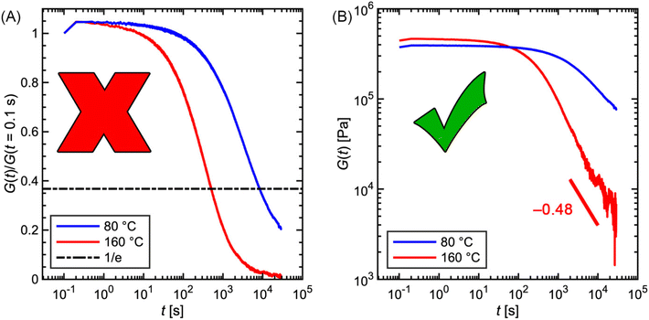Fig. 16 Comparison of polybutadiene vitrimer stress relaxation data presented in (A) normalized semi-log and (B) absolute double logarithmic formats. The black dashed line in (A) marks when the data decay to a value of 1/e. We strongly discourage plotting data in the panel A format because it grossly underestimates the terminal relaxation time of the sample. Panel B is the recommended format for plotting stress relaxation data. Data in both panels adapted from ref. 92. Copyright 2023 American Chemical Society.

The format of panel A misrepresents the viscoelastic behavior of the polybutadiene vitrimer. The normalization constant G(t = 0.1 s) is not only arbitrarily chosen, but also represents the portion of the curve that is subject to inertial artifacts. The linear y-axis overemphasizes the importance of the first decade of the modulus decay and undermines the long time data. The 1/e marking incorrectly suggests that the vitrimer reaches terminal relaxation over the course of the measurements.

In contrast to the semi-log format, the double logarithmic axes of panel B reveal a more detailed landscape of viscoelastic information. The plateau modulus regimes observed at short times indicate that the vitrimer initially behaves as a solid-like material. The absolute value of the plateau modulus provides a pathway towards estimating the cross-link density (see eqn (29)). The G(t) curves decay at longer times, but they do not exhibit the exponential shape indicative of a single mode MM, invalidating use of the 1/e criterion for estimating τ_term. Rather, the curves adopt a power law relationship with time. No features of terminal relaxation are observed, demonstrating that the vitrimer is not yet flowing like a Newtonian liquid, even after 8 h of measurement.

In general, stress relaxation, creep, and SAOS data should be plotted using double logarithmic axes to correctly capture viscoelastic behavior that occurs over time scales with different orders of magnitude. We discourage the use of semi-log or linear axes, as it risks underestimating the terminal relaxation time and greatly exaggerating the relaxation rate of a material.⁸³

4.2 Determination of terminal relaxation time

At sufficiently long times, viscoelastic liquids “flow” and LVE functions exhibit features of terminal behavior described in section 1.1.4. The terminal relaxation time τ_term is a timescale that attempts to characterize the location of this flow transition. In CAN studies, rheological experiments typically aim to connect the macroscopic flow behavior with the underlying network structure by measuring τ_term. However, several definitions of τ_term exist in the CAN literature, along with various measurement methods. The lack of a unified and rigorous protocol for evaluating τ_term in CANs inhibits identification of general guidelines for tuning their viscoelastic behavior.

To clarify the utility of measuring τ_term, it is helpful to understand the origin of these different definitions. An instructive anchor is the discrete RS {G_i,τ_i}ⁿ_i=1, which characterizes the strengths and relaxation times of the different relaxation modes. As before, the relaxation modes are arranged as τ₁ > τ₂ > … > τ_n, so that τ₁ is the longest relaxation time. Different definitions of τ_term correspond to different weighted averages of the relaxation times. Consequently, τ_term can be described using a statistical framework analogous to the one used for quantifying polymer molar mass averages.

For example, if the weight of each relaxation mode τ_i is proportional to the strength G_i, we obtain a definition based on the first moment as

τ ⁽¹⁾_term corresponds to the ratio of the viscosity and stiffness, and the superscript “(1)” indicates that it is based on the first moment. This is analogous to the number average molar mass of a polymer. In a stress relaxation experiment in which the terminal regime is reached, τ⁽¹⁾_term is formally equal to the ratio of the area under the curve divided by G(t) extrapolated to t = 0. That is

  However, G(0) is difficult to measure, and it is better to estimate τ⁽¹⁾_term from eqn (32) by first fitting a discrete RS. Thus, τ⁽¹⁾_term can be determined from either stress relaxation or SAOS measurements using this approach.

We can use the second moment of the RS to define

This is analogous to the weight average molar mass of a polymer. τ⁽²⁾_term is formally equivalent to the relaxation time τ_SS = J⁰_eη₀, which was defined using creep compliance (see eqn (16)). Since τ_SS corresponds to the second moment, it places a larger weight on longer relaxation times due to which τ⁽²⁾_term ≥ τ⁽¹⁾_term. Thus, τ⁽²⁾_term is best determined from creep and recovery measurements.

Proceeding in this fashion, we can consider a limiting case (“infinite” moment) where all the weight is placed solely on the longest relaxation time. Then

τ^(∞)_term = τ₁ (35)

This is the terminal relaxation time that is obtained from stress relaxation by calculating the slope of ln G(t) versus t in a semi-logarithmic plot, or from SAOS measurements viaeqn (21). Clearly,

τ^(∞)_term ≥ τ⁽²⁾_term ≥ τ⁽¹⁾_term (36)

As mentioned previously, the relaxation time τ_cross can be obtained from the cross-over frequency in SAOS tests. Mathematically, τ_cross ≤ τ₁. Its relationship to other moments of the RS, however, depends on the shape of the RS. For example, τ_cross is usually found to be larger than τ⁽¹⁾_term for materials that exhibit a broad RS; however, it is possible to artificially construct RS for which τ_cross < τ⁽¹⁾_term. Finally, it should be mentioned that for a single mode Maxwell model, all these different definitions of relaxation time collapse

τ⁽¹⁾_term = τ⁽²⁾_term = τ^(∞)_term = τ₁ = τ_cross (37)

Fortunately, rheology offers several techniques for determining τ_term that do not require the assumption of a single mode MM. SAOS measurements identify terminal relaxation when G′ ∝ ω² and G′′ ∝ ω¹ at low angular frequencies. If these power law scalings are observed, then τ₁ may be estimated using eqn (21). As SAOS is optimized for evaluating short time dynamics, this approach is suitable for materials that have τ₁ < 100 s. For materials with relatively slow relaxation rates, the use of creep and recovery experiments is the more appropriate method. Creep identifies terminal relaxation when the compliance J ∝ t¹. τ_SS is then calculated using eqn (16).

To aid the reader in calculating the different terminal relaxation times, the supplementary spreadsheet “Supplementary Information_Relaxation Times from Spectrum.xlsx” contains the discrete relaxation spectrum and formulas needed for analysis. Box 6 describes the stretched exponential function, an alternate model commonly used to evaluate CAN rheology.

Box 6 Stretched exponential function

The stretched exponential or Kohlrausch–Williams–Watts (KWW) function is a widely used phenomenological model for relaxation in disordered systems.^84,85 It is often used to describe stress or dielectric relaxation in polymeric systems, including CANs.^30,86,87 It takes the form

G(t) = G₀e^−(t/τ)β

where β is defined as the stretching exponent. When β = 1, the KWW function is equivalent to the single-mode Maxwell model that exhibits exponential decay. For 0 < β < 1, G(t) is “stretched out” relative to simple exponential decay, with lower values of β corresponding to a greater degree of stretching (Fig. 17). The KWW function corresponding to β > 1 is sometimes called the compressed exponential function since it decays faster than an exponential function. This case, however, is of limited practical importance.

Fig. 17 The stretched exponential function for three different values of the stretching parameter. β = 1 (blue line) corresponds to e^−t/τ. The vertical lines on the horizontal axis mark the terminal relaxation time, τ⁽¹⁾_term, for different β.

The stretched exponential function has several advantages for describing relaxation functions. It is compact and requires only a single additional parameter – the stretching exponent – to describe the broad relaxation profiles observed in numerous physical systems. It is superior to implicitly fitting a single Maxwell mode and inferring the relaxation time using the 1/e criterion. Nevertheless, some caution is necessary during use of the stretched exponential function because β is merely a convenient shortcut to specify indirectly the corresponding RS.^88,89 For small values of β, the underlying RS can extend several orders of magnitude beyond the timescale τ in the stretched exponential function. This has important consequences for inferring the terminal relaxation time in CANs. Indeed, for the KWW function the first moment terminal relaxation time is

where Γ is the Gamma function (Fig. 17). As an example, when β = 0.1, τ⁽¹⁾_term ≈ 3.6 × 10⁶τ– thus τ⁽¹⁾_term is over six orders of magnitude larger than τ. If the range of experimental data used to fit the stretched exponential function does not include τ⁽¹⁾_term, then there is some risk of incorrectly projecting observations at short timescales onto longer timescales. This concern is especially warranted for CANs because TTS often breaks down for these systems.

4.3 Alternative methods for evaluating temperature dependence of viscoelasticity

While terminal relaxation manifests as distinct fingerprints in SAOS and creep, these signatures may be challenging to observe in CANs due to their sluggish relaxation behavior. Without detecting terminal relaxation features, relaxation mechanisms cannot be precisely determined, even with the aid of a theoretical model. Nevertheless, the abundance of information provided by viscoelastic data offers additional avenues for investigating thermorheological properties.

4.3.1 Cross-over relaxation time from SAOS. Perhaps the most discernible feature in SAOS data is the cross-over point between G′ and G′′, i.e., . The angular frequency at which cross-over occurs may be translated to τ_crossvia the relationship . The temperature dependence of τ_cross offers insight into the molecular principles that control CAN viscoelasticity.

Fig. 18 highlights some literature examples that demonstrate the utility of τ_cross for investigating associative and dissociative CANs. Porath and Evans measured τ_cross for telechelic polydimethysiloxane vitrimers with boronic acid cross-links (Fig. 18A and B). For all cross-link densities, the authors found that τ_cross followed an Arrhenius relationship with an activation energy of approximately 30 kJ mol⁻¹. τ_cross was systematically larger than the relaxation times estimated using the 1/e criterion.³⁸ In another case, Adzima et al. related τ_cross = 1/ω_cross to the sol–gel transition of a polymer network bearing dissociative Diels–Alder cross-links (Fig. 18C). At 87 °C, 5 °C below the gel point temperature, τ_cross ≈ 2.5 s. As the temperature was increased to 91 °C, τ_cross decreased to approximately 1 s, indicating the acceleration of network dynamics. As the temperature was further increased beyond the gel point temperature to 95 °C, τ_cross shifted to a low value outside the measured angular frequency range.⁹⁰

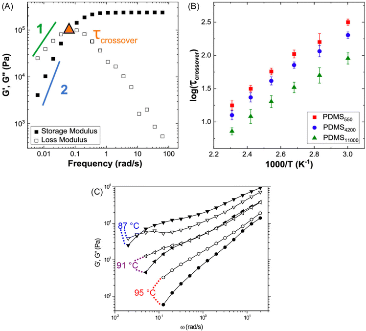Fig. 18 (A) SAOS and (B) Arrhenius plot of cross-over time versus inverse temperature for PDMS vitrimers. In (A), cross-over frequency and terminal relaxation scalings are identified. Adapted from ref. 38. Copyright 2021 American Chemical Society. (C) SAOS of a dissociative Diels–Alder polymer network below (87 °C), slightly below (91 °C), and above (95 °C) the gel point temperature. Filled and open symbols represent G′ and G′′, respectively. Adapted from ref. 90. Copyright 2008 American Chemical Society.

4.3.2 Time–temperature superposition on CANs. TTS is an especially powerful tool for studying polymer dynamics. Through systematic measurements at varying temperature, viscoelastic behavior can be investigated at time scales not normally accessible by experiment. While useful, TTS rigorously applies only to systems that are thermorheologically simple. For CANs, in which the backbone dynamics and cross-link kinetics have inherently different thermoresponsiveness, this assumption is violated. However, prudent application of TTS analyses can still clarify mechanisms that control viscoelasticity.

Fig. 19 shows some examples of TTS applied to CAN rheology data. Sheridan and Bowman attempted to apply TTS to the SAOS data of a dissociative Diels–Alder polymer network near its sol–gel transition temperature (Fig. 19A and B). The angular frequencies were shifted by dividing them by ω_cross, while G′ and G′′ were normalized by the magnitude of the moduli at cross-over. This normalization scheme exhibited superposition at frequencies below and near ω_cross, but did not overlap the data at higher frequencies. This failure of TTS suggested that the dynamics of the percolating network and sol clusters had distinct temperature dependences.⁹¹

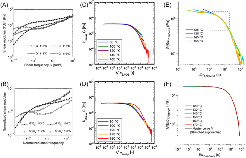Fig. 19 Examples of time–temperature superposition for CAN systems. (A) Raw and (B) shifted SAOS data for a polymer network with dissociative Diels–Alder cross-links. Adapted from ref. 91. Copyright 2012 American Chemical Society. (C) and (D) demonstrate polybutadiene vitrimer stress relaxation superposed using shift factors determined from other experiments. (C) SAOS shift factors a_SAOS used. (D) Creep shift factors a_creep used. Adapted from ref. 92. Copyright 2023 American Chemical Society. (E) Polystyrene CAN with dissociative cross-links. (F) Aliphatic CAN with associative cross-links. Adapted from ref. 93. Copyright 2020 American Chemical Society.

Fig. 19C and D focus on recent work by the authors of this tutorial review, in which we investigated the linear rheology of polybutadiene vitrimers through the lens of TTS. SAOS and creep data were superposed into master curves using two different sets of horizontal shift factors (a_SAOS and a_creep, respectively). Although both exhibited Arrhenius relationships with temperatures, a_creep had a significantly larger activation energy than a_SAOS. When applied to stress relaxation data, a_SAOS and a_creep separately collapsed the short and long time data. Based on this result, the short time dynamics were assigned to represent segmental motions of the polybutadiene backbone, while the long time dynamics were hypothesized to reflect the interplay among network strand relaxations, cross-link exchange, and cross-link mobility within the vitrimer matrix.⁹²

Fig. 19E and F detail stress relaxation master curves of two different CAN systems. Panel E centers on a styrenic network with benzylic 1,2,3-triazolium cross-links that engage in a two-step trans-N-alkylation dissociative exchange. G_XL and τ_cross each decrease with temperature, causing both the vertical and horizontal shift factors to obey Arrhenius relationships. Application of the SAOS shift factors on stress relaxation data, however, collapses only a narrow region of the curve. Panel F concentrates on an aliphatic network that also has 1,2,3-triazolium cross-links, but its G_XL is constant between 120 to 170 °C. Consequently, its rheological behavior approximates that of an associative CAN. The stress relaxation data for this material superposed over a wide time range.⁹³

4.3.3 Relaxation spectra for CANs. The various LVE protocols offer separate but complementary views of the RS by weighing the relaxation processes differently. Thus, the RS plays two important roles in linear rheology: (I) it offers a convenient basis for interconversion between different LVE functions, and (II) it decomposes the output of a standard rheological test into individual contributions by characterizing the timescale and intensity associated with different relaxation processes. Both roles have important ramifications for the study of CANs.

As mentioned previously, CANs are not thermorheologically simple. This complicates the application of TTS and limits the window of timescales or frequencies over which the material response can be characterized. One option for expanding the observation window that does not rely on TTS is to extract and merge the RS inferred from measurements using different experimental protocols. To our knowledge, this approach has not been explored much – for CANs or otherwise – although methods and tools to perform such analysis are available.^49,50,94 This may be a fruitful direction for future research on CAN viscoelasticity.

Fig. 20 highlights a few studies that have used the RS to get a direct understanding of CAN relaxation processes. Porath et al. compared the RS of equimolar mixtures of components with different boric acid cross-link chemistry (Fig. 20A). They found that the fast component controls the overall rheology of the mixtures. This is visually evident in Fig. 20A, as the RS of the mixture is pulled closer to the RS of the fast component (PDMS-BA) compared to the slow component (PDMS-NbDBA). The response of these networks differed from other studies of mixtures of CANs where multiple peaks corresponding to the two components remained distinct. The authors speculated that the telechelic nature of the networks – i.e., cross-link junctions occur at both ends of the chains – may be responsible for the observed difference.^95,96Fig. 20B, originally published in the ESI of ref. 97, illustrates how the distribution of cross-links on the chain affects the RS. When cross-links were distributed uniformly, the RS had a single peak. However, when cross-links were attached to only one block of a block copolymer, a qualitatively different RS was observed in which the presence of a distinct and slow relaxation process, a small fraction of permanent cross-linking, or both could be ascertained.⁹⁷

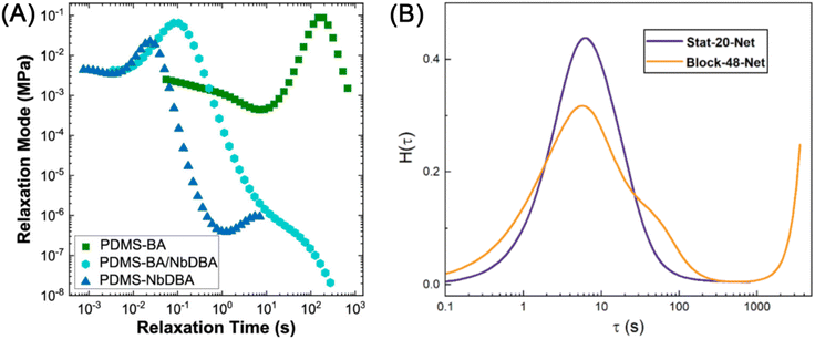Fig. 20 (A) Discrete relaxation spectra of poly(dimethylsiloxane) vitrimers with varying boric acid cross-link chemistry. Adapted from ref. 95. Copyright 2022 American Chemical Society. (B) Continuous relaxation spectra of acrylic vitrimers in which the cross-links are distributed in a statistical or blocky manner. Adapted from ref. 97. Copyright 2021 American Chemical Society.

Nevertheless, a few caveats regarding the use of RS are in order. First, LVE experiments probe relaxation timescales over a finite temporal window. The RS extracted from such measurements inherits this trait, and is necessarily incomplete as a consequence. Second, the discrete RS is not unique, and therefore, it is important not to over-interpret the individual weights and timescales. The terminal relaxation times based on the first and second moments of the discrete RS (section 4.2) are relatively stable, so long as the terminal regime is reached in the underlying stress relaxation or SAOS measurements. However, the same is not true for the longest relaxation time which is sensitive to the width of the experimental window, and the method used to calculate the discrete RS.

5. Summary and outlook

Over the past 100 years, linear rheology has played a pivotal role in decoding the relationship between the chemical structures of polymers and their macroscopic viscoelasticity. Through standardized experiments, it enables systematic examination of how the solid-like and liquid-like characteristics of polymers evolve across various time scales. The rigorous foundation formed by the pairing of experiment and theory was essential for creating the thorough understanding of classical thermoplastic and thermoset rheology that we have today. As we delve into the modern age of CAN materials, this well-established framework becomes indispensable.

Specifically, linear rheology offers many pathways towards investigating the impact of dynamic covalent chemistry on polymers. The trinity of stress relaxation, creep and recovery, and SAOS identifies relaxation modes that occur over a wide range of time scales. Discrete or continuous relaxation spectra provide a visual representation of these modes. Investigating the temperature dependence of terminal relaxation grants access towards quantifying the flow activation energy. Even in the absence of terminal relaxation, the use of a time–temperature superposition analysis may reveal different thermal dependences among the various relaxation modes.

While linear rheology is critical for studying the physical chemistry of CANs, the use of the technique alone is not sufficient for developing a comprehensive understanding. Because of the small strains that are applied, linear rheology only probes the viscoelastic behavior of polymers at rest. Nonlinear rheology measurements are needed to evaluate behavior under actual processing conditions. Furthermore, rheology can only suggest that a structural change has occurred, it does not actually reveal what the structure is. Generally, rheology is best when complemented by other experimental methods that directly characterize structure, such as scattering and microscopy.

Despite the initial learning curve, linear rheology is instrumental in elucidating the impact of dynamic covalent chemistry on CANs. Our goal with this tutorial review is to equip readers with fundamental tools not only to navigate the rheology literature, but also to craft experiments for evaluating their own unique materials. Numerous challenges persist in developing a complete understanding of the relationship between dynamic covalent chemistry and viscoelasticity. We firmly advocate that an intimate combination of synthesis, experiment, and theory is the essential approach for expanding our existing polymer rheology framework to encompass CANs.

Abbreviations

BSP	Boltzmann superposition principle
CAN	Covalent adaptable network
LVE	Linear viscoelasticity or linear viscoelastic
MM	Maxwell model
PS	Polystyrene
RS	Relaxation spectrum
SAOS	Small-amplitude oscillatory shear
TTS	Time–temperature superposition

Symbols

a T	Horizontal shift factor for time–temperature superposition
b T	Vertical shift factor for time–temperature superposition
G g	Glassy modulus
G 0	Shear modulus
G i	Modulus of the ith Maxwell mode
G Rouse	Modulus corresponding to the Rouse model
G ∞	Equilibrium shear modulus
G min	Minimum detectable modulus
G ^0 N	Plateau modulus contribution due to entanglements
G XL	Plateau modulus contribution due to cross-links
G(t)	Shear stress relaxation modulus
G′	Storage modulus
G′′	Loss modulus
G*(ω)	Complex shear modulus
H	Height of sample in a rheometer
J(t)	Creep compliance
N	Number of statistical segments per chain
γ	Shear strain
	Shear strain rate
η 0	Zero-shear viscosity
η i	Viscosity of the ith Maxwell mode
K τ	Sample geometry constant
J ^e0	Steady-state creep compliance
J rec	Recoverable compliance
σ	Shear stress
σ e	Elastic shear stress
σ v	Viscous shear stress
τ term	Terminal relaxation time
τ i	Relaxation time of the ith Maxwell mode
τ SS	Steady-state flow relaxation time
τ cross	Relaxation time based on the cross-over frequency
τ Rouse	Terminal relaxation time of the Rouse model
T ref	Reference temperature for time–temperature superposition
v top	Velocity of sample top layer during simple shear experiment
ω	Angular frequency
ω cross	Cross-over frequency at which G′ = G′′
γ crit	Critical strain above which nonlinear effects manifest

Conflicts of interest

There are no conflicts to declare.

Appendix: Experimental details of commercial polystyrene rheology measurements

Commercial polystyrene (PS, M_n = 220 kg mol⁻¹ and Đ = 1.61 based on light scattering) was sourced from Sigma Aldrich. Linear rheology assessments of PS were carried out using an Anton Paar MCR 302e rotational rheometer equipped with parallel plates geometry. The upper and lower geometries consisted of 25 mm stainless steel plates, with the lower plate featuring Peltier temperature control. To mitigate thermal degradation, the plate geometry was enclosed in a hood with a continuous 200 L h⁻¹ nitrogen flow. Temperature control was maintained with an accuracy of ±0.1 °C. An applied normal force ranging from 0.1 to 1 N facilitated contact between the PS sample and the parallel plates. PS discs (25 mm diameter and 2 mm thickness) were fashioned using stainless steel frames subjected to an applied load of 3 tons at 150 °C for 8 min.

Strain amplitude sweeps, small-amplitude oscillatory shear (SAOS), stress relaxation, and creep and recovery tests were conducted on the PS. As illustrated in Fig. 11A, the linear viscoelastic regime was determined at temperatures of 130 and 190 °C. For SAOS and stress relaxation, measurements on fresh samples were performed using an applied strain within the identified linear viscoelastic regimes at 130 and 190 °C.

The experimental protocol for PS rheology measurements involved placing the sample disc onto the preheated lower plate at 195 °C. The upper plate and Peltier hood were then slowly lowered onto the sample to create a plate gap of approximately 2 mm. The sample was cooled at a rate of 1 °C min⁻¹ to 190 °C and annealed for a period of 15 min. Following the annealing period, either SAOS, stress relaxation, or creep and recovery measurements were conducted. Subsequent measurements at 175, 160, 145, and 130 °C followed similar protocols, with increased annealing times to accommodate the slower polymer dynamics.

Acknowledgements

We would like to thank Prof. Hans Heuts for strongly encouraging us to write this tutorial review. We would like to thank Prof. Joseph Schlenoff, Daniel Barzycki, Marie Chmara, and Dana Ezzeddine for reviewing drafts of this manuscript and providing helpful feedback. We are very grateful to Prof. Rebekah Sweat and the Sweat Laboratory for use of their rheometer for photographing commercial polyisoprene measurements. We are very grateful to Prof. Justin Kennemur and the Kennemur Laboratory for use of their size-exclusion chromatography instrument. This work was supported primarily by the National Science Foundation (DMR-2144007, DMR-1727870). This work was partially supported by funds provided by the Oak Ridge Associated Universities Foundation, ORAU-Directed Research and Development Program. This work also was partially supported by the 3M Non-Tenured Faculty Award. This work also was supported using start-up funds from Florida State University and the Florida A&M University – Florida State University College of Engineering. SS would like to acknowledge support from the Department of Scientific Computing at Florida State University, and helpful discussions with Prof. Yogesh M. Joshi.

References

1. D. Hosler, S. L. Burkett and M. J. Tarkanian, Science, 1999, 284, 1988–1991,  DOI:10.1126/science.284.5422.1988.
2. M. J. Tarkanian, PhD thesis, Massachusetts Institute of Technology, 2003.
3. M. J. Tarkanian and D. Hosler, Lat. Am. Antiq., 2011, 22, 469–486,  DOI:10.7183/1045-6635.22.4.469.
4. M. Thurner and J. Pimentel, New World Objects of Knowledge: A Cabinet of Curiosities, University of London Press, London, 2021.
5. H. L. Fisher, Ind. Eng. Chem., 1939, 31, 1381–1389,  DOI:10.1021/ie50359a015.
6. C. Guise-Richardson, Technol. Cult., 2010, 51, 357–387,  DOI:10.1353/tech.0.0437.
7. L. H. Baekeland, J. Ind. Eng. Chem., 1909, 1, 149–161,  DOI:10.1021/ie50003a004.
8. H. A. Bruson and H. Staudinger, Ind. Eng. Chem., 1926, 18, 381–383,  DOI:10.1021/ie50196a013.
9. B. Veldman, T. Kaully, R. K. Feller, E. Falcao and F. Wudl, Macromolecules, 2009, 42, 6848–6850,  DOI:10.1021/ma901123p.
10. F. Wudl, in Hierarchical Macromolecular Structures: 60 Years after the Staudinger Nobel Prize I, ed. V. Percec, Springer, 2013, vol. 1, ch. 12, pp. 211–216.
11. L. Imbernon and S. Norvez, Eur. Polym. J., 2016, 82, 347–376,  DOI:10.1016/j.eurpolymj.2016.03.016.
12. J. M. Garcia and M. L. Robertson, Science, 2017, 358, 870–872,  DOI:10.1126/science.aaq0324.
13. D. K. Schneiderman and M. A. Hillmyer, Macromolecules, 2017, 50, 3733–3749,  DOI:10.1021/acs.macromol.7b00293.
14. T. Yan, A. H. Balzer, K. M. Herbert, T. H. Epps and L. T. J. Korley, Chem. Sci., 2023, 14, 5243–5265,  10.1039/d3sc00551h.
15. C. J. Kloxin and C. N. Bowman, Chem. Soc. Rev., 2013, 42, 7161–7173,  10.1039/c3cs60046g.
16. W. Zou, J. Dong, Y. Luo, Q. Zhao and T. Xie, Adv. Mater., 2017, 29, 1606100,  DOI:10.1002/adma.201606100.
17. G. M. Scheutz, J. J. Lessard, M. B. Sims and B. S. Sumerlin, J. Am. Chem. Soc., 2019, 141, 16181–16196,  DOI:10.1021/jacs.9b07922.
18. J. M. Winne, L. Leibler and F. E. D. Prez, Polym. Chem., 2019, 10, 6091–6108,  10.1039/c9py01260e.
19. M. K. McBride, B. T. Worrell, T. Brown, L. M. Cox, N. Sowan, C. Wang, M. Podgorski, A. M. Martinez and C. N. Bowman, Annu. Rev. Chem. Biomol. Eng., 2019, 10, 1–24,  DOI:10.1146/annurev-chembioeng-060718-030217.
20. V. Zhang, B. Kang, J. V. Accardo and J. A. Kalow, J. Am. Chem. Soc., 2022, 144, 22358–22377,  DOI:10.1021/jacs.2c08104.
21. L. Porath, B. B. Jing and C. M. Evans, ACS Macro Lett., 2022, 11, 475–483,  DOI:10.1021/acsmacrolett.2c00038.
22. F. Tanaka, Polymer Physics: Applications to Molecular Association and Thermoreversible Gelation, Cambridge University Press, 2011.
23. S. Wu and Q. Chen, Macromolecules, 2022, 55, 697–714,  DOI:10.1021/acs.macromol.1c01605.
24. T. Katashima, Nihon Reoroji Gakkaishi, 2022, 50, 51–56,  DOI:10.1678/rheology.50.51.
25. M. Ahmadi, A. Hanifpour, S. Ghiassinejad and E. van Ruymbeke, Chem. Mater., 2022, 34, 10249–10271,  DOI:10.1021/acs.chemmater.2c02853.
26. M. Hayashi, Nihon Reoroji Gakkaishi, 2022, 50, 15–20,  DOI:10.1678/rheology.50.15.
27. S. S. Velankar and D. Giles, Rheol. Bull., 2007, 76, 8–20.
28. F. J. Stadler, Korea-Aust. Rheol. J., 2014, 26, 277–291,  DOI:10.1007/s13367-014-0032-2.
29. H. Ramli, N. F. A. Zainal, M. Hess and C. H. Chan, Chem. Teach. Int., 2022, 4, 307–326,  DOI:10.1515/cti-2022-0010.
30. M. L. Martins, X. Zhao, Z. Demchuk, J. Luo, G. P. Carden, G. Toleutay and A. P. Sokolov, Macromolecules, 2023, 56, 8688–8696.
31. R. P. Chartoff, J. D. Menczel and S. H. Dillman, Dynamic Mechanical Analysis (DMA), in Thermal Analysis of Polymers: Fundamentals and Applications, 2009, pp. 387–495.
32. F. A. Morrison, Understanding Rheology, Oxford University Press, New York, New York, 2001.
33. C. W. Macosko, Rheology: Principles, Measurements, and Applications, VCH, Germany, 1994.
34. T. Mezger, The Rheology Handbook, Vincentz Network, Hanover, Germany, 2020.
35. R. Edgeworth, B. J. Dalton and T. Parnell, Eur. J. Phys., 1984, 5, 198–200,  DOI:10.1088/0143-0807/5/4/003.
36. R. G. Larson, The Structure and Rheology of Complex Fluids, Oxford University Press, New York, New York, 1999.
37. J. W. Goodwin and R. W. Hughes, Rheology for Chemists: An Introduction, RSC Publishing, United Kingdom, 2008.
38. L. E. Porath and C. M. Evans, Macromolecules, 2021, 54, 4782–4791,  DOI:10.1021/acs.macromol.0c02800.
39. J. Lee, B. B. Jing, L. E. Porath, N. R. Sottos and C. M. Evans, Macromolecules, 2020, 53, 4741–4747,  DOI:10.1021/acs.macromol.0c00784.
40. S. W. Provencher, J. Chem. Phys., 1976, 64, 2772–2777,  DOI:10.1063/1.432601.
41. S. W. Provencher, Comput. Phys. Commun., 1982, 27, 229–242,  DOI:10.1016/00104655(82)90174-6.
42. J. Honerkamp and J. Weese, Rheol. Acta, 1993, 32, 65–73,  DOI:10.1007/BF00396678.
43. H. H. Winter, J. Non-Newtonian Fluid Mech., 1997, 68, 225–239,  DOI:10.1016/S0377-0257(96)01512-1.
44. S. Shanbhag, Macromol. Theory Simul., 2019, 8, 1900005,  DOI:10.1002/mats.201900005.
45. S. Shanbhag, Rheol. Acta, 2020, 59, 509–520,  DOI:10.1007/s00397-020-01212-w.
46. Blind Men Appraising an Elephant, https://asia.si.edu/explore-art-culture/collections/search/edanmdm:fsg_F2019.3.34a-f/ (accessed September 2023).
47. W. Voigt, Ann. Phys., 1892, 283, 671–693,  DOI:10.1002/andp.18922831210.
48. W. Thomson, Proc. R. Soc. London, Ser. A, 1865, 14, 289–297 https://www.jstor.org/stable/112142 .
49. D. W. Mead, J. Rheol., 1994, 38, 1769–1795,  DOI:10.1122/1.550526.
50. R. J. Loy, F. R. de Hoog and R. S. Anderssen, J. Rheol., 2015, 59, 1261–1270,  DOI:10.1122/1.4929398.
51. K. Ninomiya, J. Phys. Chem., 1963, 67, 1152–1152,  DOI:10.1021/j100799a502.
52. Q. Chen, H. Masser, H.-S. Shiau, S. Liang, J. Runt, P. C. Painter and R. H. Colby, Macromolecules, 2014, 47, 3635–3644,  DOI:10.1021/ma5008144.
53. G. Schramm, A Practical Approach to Rheology and Rheometry, Thermo Electron, Germany, 2004.
54. J. D. Ferry, Viscoelastic Properties of Polymers, Wiley, United Kingdom, 1980.
55. M. O. Marasteanu and D. A. Anderson, Transp. Res. Rec., 2000, 1728, 1–6,  DOI:10.3141/1728-01.
56. H. Münstedt, J. Rheol., 2014, 58, 565–587,  DOI:10.1122/1.4866049.
57. R. G. Ricarte, F. Tournilhac, M. Cloître and L. Leibler, Macromolecules, 2020, 53, 1852–1866,  DOI:10.1021/acs.macromol.9b02415.
58. M. Rubinstein and R. H. Colby, Polymer Physics, Oxford University Press, United Kingdom, 2003.
59. T. P. Lodge and P. C. Hiemenz, Polymer Chemistry, CRC Press, Taylor & Francis Group, United Kingdom, 2020.
60. L.-I. Palade, V. Verney and P. Attané, Macromolecules, 1995, 28, 7051–7057,  DOI:10.1021/ma00125a003.
61. L.-I. Palade, V. Verney and P. Attané, Rheol. Acta, 1996, 35, 265–273,  DOI:10.1007/bf00366913.
62. D. J. Plazek, J. Rheol., 1996, 40, 987–1014,  DOI:10.1122/1.550776.
63. R. Cross, Am. J. Phys., 2012, 80, 870–875,  DOI:10.1119/1.4732086.
64. R. G. Larson, S. Goyal and C. Aloisio, Rheol. Acta, 1996, 35, 252–264,  DOI:10.1007/BF00366912.
65. M. J. Webber and M. W. Tibbitt, Nat. Rev. Mater., 2022, 7, 541–556,  DOI:10.1038/s41578-021-00412-x.
66. P. Grootenhuis, J. Sound Vib., 1970, 11, 421–433,  DOI:10.1016/S0022-460X(70)80004-9.
67. C. Chen and R. Lakes, Int. J. Solids Struct., 1990, 26, 1313–1328,  DOI:10.1016/0020-7683(90)90081-6.
68. S. Paje, M. Bueno, F. Terán, R. Miró, F. Pérez-Jiménez and A. Martínez, Appl. Acoust., 2010, 71, 578–582,  DOI:10.1016/j.apacoust.2009.12.003.
69. Modular Compact Rheometer: MCR 102e/302e/502e, https://www.anton-paar.com/us-en/products/details/rheometer-mcr-102-302-502/?sku=241353 (accessed September 2023).
70. Discovery HR 30, https://www.tainstruments.com/hr-30/ (accessed September 2023).
71. R. H. Ewoldt, M. T. Johnston and L. M. Caretta, in Complex Fluids in Biological Systems, ed. S. Spagnolie, Springer, 2015, vol. 1, ch. 6, pp. 207–241.
72. G. Filippone, S. C. Carroccio, R. Mendichi, L. Gioiella, N. T. Dintcheva and C. Gambarotti, Polymer, 2015, 72, 134–141,  DOI:10.1016/j.polymer.2015.06.059.
73. K. Liu, S. Ronca, E. Andablo-Reyes, G. Forte and S. Rastogi, Macromolecules, 2015, 48, 131–139,  DOI:10.1021/ma501729y.
74. C. R. Arza, P. Jannasch, P. Johansson, P. Magnusson, A. Werker and F. H. J. Maurer, J. Appl. Polym. Sci., 2015, 132, 41836,  DOI:10.1002/app.41836.
75. A. Fazlali, V. G. Khondabi, M. J. Sharifi and M. A. Nikoohemmat, Int. J. Ind. Chem., 2019, 10, 49–55,  DOI:10.1007/s40090-019-0170-y.
76. J. L. Schrag, Trans. Soc. Rheol., 1977, 21, 399–413,  DOI:10.1122/1.549445.
77. R. H. Ewoldt and G. H. McKinley, Rheol. Bull., 2007, 76, 4–24.
78. Tips and Tricks from Joe Flow – Normal Force Control: May the Force Be with You, https://crmdocs.anton-paar.com/crm/crmdocdownload.nsf/0/C4C28890D95CBDE2C12586FA001CEB89/$file/XRRIA019EN-B_Joe_Flow_normal_force_control.pdf, (accessed November 2023).
79. H. Gevgilili and D. M. Kalyon, J. Rheol., 2001, 45, 467–475,  DOI:10.1122/1.1339248.
80. L. A. Archer, Y.-L. Chen and R. G. Larson, J. Rheol., 1995, 39, 519–525,  DOI:10.1122/1.550710.
81. V. Mhetar and L. A. Archer, Macromolecules, 1998, 31, 6639–6649,  DOI:10.1021/ma971339h.
82. S. G. Hatzikiriakos, Prog. Polym. Sci., 2012, 37, 624–643,  DOI:10.1016/j.progpolymsci.2011.09.004.
83. R. G. Ricarte and S. Shanbhag, Macromolecules, 2021, 54, 3304–3320,  DOI:10.1021/acs.macromol.0c02530.
84. R. Kohlrausch, Ann. Phys., 1854, 167, 179–214,  DOI:10.1002/andp.18541670203.
85. G. Williams and D. C. Watts, Trans. Faraday Soc., 1970, 66, 80–85,  10.1039/tf9706600080.
86. J. C. Phillips, Rep. Prog. Phys., 1996, 59, 1133,  DOI:10.1088/0034-4885/59/9/003.
87. J. C. Phillips, J. Non-Cryst. Solids, 2011, 357, 3853–3865,  DOI:10.1016/j.jnoncrysol.2011.08.001.
88. D. C. Johnston, Phys. Rev. B: Condens. Matter Mater. Phys., 2006, 74, 184430,  DOI:10.1103/physrevb.74.184430.
89. J. C. Mauro and Y. Z. Mauro, Phys. A, 2018, 506, 75–87,  DOI:10.1016/j.physa.2018.04.047.
90. B. J. Adzima, H. A. Aguirre, C. J. Kloxin, T. F. Scott and C. N. Bowman, Macromolecules, 2008, 41, 9112–9117,  DOI:10.1021/ma801863d.
91. R. J. Sheridan and C. N. Bowman, Macromolecules, 2012, 45, 7634–7641,  DOI:10.1021/ma301329u.
92. R. G. Ricarte, S. Shanbhag, D. Ezzeddine, D. Barzycki and K. Fay, Macromolecules, 2023, 56, 6806–6817,  DOI:10.1021/acs.macromol.3c00883.
93. A. Jourdain, R. Asbai, O. Anaya, M. M. Chehimi, E. Drockenmuller and D. Montarnal, Macromolecules, 2020, 53, 1884–1900,  DOI:10.1021/acs.macromol.9b02204.
94. S. Shanbhag, J. Rheol., 2023, 67, 965–975,  DOI:10.1122/8.0000695.
95. L. Porath, J. Huang, N. Ramlawi, M. Derkaloustian, R. H. Ewoldt and C. M. Evans, Macromolecules, 2022, 55, 4450–4458,  DOI:10.1021/acs.macromol.1c02613.
96. B. M. El-Zaatari, J. S. A. Ishibashi and J. A. Kalow, Polym. Chem., 2020, 11, 5339–5345,  10.1039/d0py00233j.
97. J. S. A. Ishibashi, I. C. Pierce, A. B. Chang, A. Zografos, B. M. El-Zaatari, Y. Fang, S. J. Weigand, F. S. Bates and J. A. Kalow, Macromolecules, 2021, 54, 3972–3986,  DOI:10.1021/acs.macromol.0c02744.

---

Footnote

† Electronic supplementary information (ESI) available. See DOI: https://doi.org/10.1039/d3py01367g

---