
Ultrafast processes: coordination chemistry and quantum theory
Chantal
Daniel

Laboratoire de Chimie Quantique, Université de Strasbourg, CNRS UMR7177, Institut Le Bel, 4 Rue Blaise Pascal, 67000 Strasbourg, France. E-mail: c.daniel@unistra.fr
First published on 18th November 2020
Abstract
Coordination compounds, characterized by fascinating and tunable electronic properties, are capable of binding easily to proteins, polymers, wires and DNA. Upon irradiation, these molecular systems develop functions finding applications in solar cells, photocatalysis, luminescent and conformational probes, electron transfer triggers and diagnostic or therapeutic tools. The control of these functions is activated by the light wavelength, the metal/ligand cooperation and the environment within the first picoseconds (ps). After a brief summary of the theoretical background, this perspective reviews case studies, from 1st row to 3rd row transition metal complexes, that illustrate how spin–orbit, vibronic coupling and quantum effects drive the photophysics of this class of molecules at the early stage of the photoinduced elementary processes within the fs–ps time scale range.
1 Introduction
Electronic excited state decay in transition metal complexes started to be discussed in the 70s1 in terms of radiative/non-radiative processes, quantum yields and lifetimes. Very soon, the role of intersystem crossing was found to be very important on the basis of strong spin–orbit coupling (SOC) effects induced by the presence of heavy metal atoms.2 The earlier studies were mainly dedicated to molecules with a long-lived triplet excited state responsible for phosphorescence, such as Ru(II), Pt(II) and Ir(III) complexes obtained by direct metalation of an organic chromophore,3 bodipy being the most famous one.4 Investigation of radiative vs. non-radiative decay on the basis of Kasha's and El-Sayed's rules and the energy gap law was the norm following the success of these early concepts in interpreting the photophysics of organic molecules on the basis of almost pure S1/T1 electronic states within a weak coupling limit (Scheme 1(a)). This approach is still successful for coordination compounds specifically designed to avoid a high density of nearly degenerate low-lying excited states, important nuclear relaxation, strong coupling and large electronic mixing.5 Interpretation of the photophysics has been safely based on steady-state spectroscopies and single-determinant computational approaches focusing on the electronic and structural properties of the S0 ground state and S1/T1 excited states6 within either the metal-to-ligand-charge-transfer (MLCT) model or the intra-ligand (IL) model considering multi-step 100% ultrafast decay to S1.7 Refined zero magnetic field splitting studies varying the chemical environment, the temperature and the pressure can be performed for a quantitative assessment of SOC effects and a deep understanding of the photophysics.8 | ||
| Scheme 1 (a) Luminescence decay based on the two-state model. (b) Cartoon of the typical radiative and non-radiative decays in coordination compounds. | ||
When designing coordination compounds for specific functions and applications, the main concern is to tailor the photophysical properties by varying the metal center(s), the ligands and the environment in order to obtain large quantum yields and a palette of bright colors, efficient intersystem crossing (ISC) quantum yields, and various kinetics and time-scales.9 The probability of getting back to the S1/T1 “ideal” situation described above, allowing the use of simple techniques and concepts developed in the 60–70s for organic chromophores, is very low. Indeed, most of the time, the systems are characterized by a high density of excited states, nearly degenerate low-lying excited states of mixed character opening the route to a number of channels of deactivation of various time-scales before reaching the lowest long-lived T1 state (Scheme 1(b)).
Sophisticated time-resolved spectroscopies, sometimes supplemented by time-resolved X-ray absorption techniques, are mandatory to decipher the electronic excited state decays inherently linked to nuclear relaxation within the ps–fs time-scales.10
This is illustrated by recent studies dedicated to the 1st, 2nd and 3rd row transition metal complexes involved in chemical catalysis and biochemical processes,11 in metal-based charge transfer chromophores,12 phosphorescent materials for OLEDs,13 photosensitizers and photocatalysts,14 and metallophilic oligomers designed for functional molecular assemblies and light-emitting devices.15 Cu(I) complexes, characterized by large photoinduced structural changes in the low-lying electronic excited states, have motivated a number of illuminating experimental and theoretical studies.16 The ultimate goal of this field of research is to control the excited state dynamics by means of tailored pulses that manipulate the vibrations of the molecules to regulate the population of the key electronic states for specific processes (luminescence decay, ultrafast electron transfer at long distances, selective dissociation, thermally activated delay fluorescence (TADF), etc.).17
In parallel, theoretical investigations need robust and highly correlated electronic structure theory able to determine the molecular structure of both ground and low-lying excited states and to describe on the same footing various electronic states, namely metal-centered (MC), MLCT, IL, ligand-to-ligand charge transfer (LLCT), and ligand-to-metal charge transfer (LMCT) states of mixed character, relativistic, solvent and SOC effects. Ultimately, simulation of the evolution of the molecular states in real time by means of non-adiabatic quantum dynamics or semi-classical trajectories including SOC effects should give access to observables (time-resolved spectra, quantum yields, time-scales, etc.).
This perspective based on recent research in the field of coordination chemistry is organized as follows: the theoretical background is summarized in the next section with presentation of the most recent electronic structure methods available for providing excited state structures, transition energies, and spin and vibronic couplings subsequently used in molecular dynamics or wavepacket simulations. Then, case studies reporting the simulation of excited state non-adiabatic dynamics of the 1st row to 3rd row transition metal complexes illustrate how spin–orbit and vibronic couplings and quantum effects drive the photophysics of this class of molecules at the early stage of the photoinduced elementary processes within the fs–ps time scale range.
2 Theoretical background
2.1 Electronic structure theory
The density matrix renormalization group (DMRG) method,32 with more favorable scaling, allows the inclusion of about one hundred correlated electrons in one hundred active orbitals. In its automated version, based on iterative entanglement measures,33 a diagrammatic representation of the static correlation between each pair of orbitals and how their occupation diverges from 0 or 2 facilitates the choice of the active space without any a priori knowledge. Whereas CASPT2 calculations performed on top of limited CASSCF wavefunctions lead to results of limited value, its extension to a larger active space by using DMRG as the solver gives quantitative results for transition metal complexes, as shown recently.34
The drawbacks of TD-DFT in the context of excited state coordination chemistry are twofold: (i) the electronic diversity and flexibility of this class of molecules are not compatible with the approximations and limitations of the method; (ii) applying solvent or relativistic corrections by approximate approaches within the framework of an approximate method may result in a total misunderstanding of the physics and prevents any robust interpretation both of the calculated properties and defects of the method itself. Whereas developing hundreds of more and more sophisticated functionals35 may help to approach a realistic solution for the ground state physical system, the task would be titanic and useless for the excited states because of their diversity.36 The next breakthrough will certainly come from excited state specific methods developed within a hybrid DFT/wavefunction formalism, such as multiconfiguration pair-DFT (MC-PDFT)37 or DFT-multireference CI (DFT-MRCI).38 Nevertheless, TD-DFT and satellite developments39 are able to treat a number of problems related to excited-state coordination chemistry and most of the time result in appropriate qualitative insights. This contributes to the charm of the method provided that the conclusions are related to reliable experimental data and/or accurate ab initio results with a careful emphasis on the interpretation.40
| H(Q) = (TN + V0(Q))Π + W(Q) |
Most of the electronic structure theories described above provide electronic ground state to excited state transition energies, the gradient of the energy, the Hessian and the SOC—critical data for the construction of the W(Q) matrix.
Multiplet states, more particularly triplet states, govern the photophysics of coordination compounds,43 and SOC plays a key role in intersystem crossing, phosphorescence, TADF, singlet fission phenomena and magnetic properties.7,44 At the TD-DFT level of theory, SOC is perturbationally computed either within the relativistic two-component zero-order regular approximation ZORA scheme45 or according to more sophisticated methods.46 In multiconfiguration wavefunction approaches, SOC is often included a posteriori based on the concept of interacting electronic states via SOC using a part of the Douglas-Kroll Hamiltonian47 within the one-electron effective Hamiltonian scheme.48 A number of approximate SOC operators have been developed for practical use in molecular quantum chemistry and introduced either perturbationally or variationally in electronic structure theory.49
The intrastate κ(n)i and inter-state linear λ(nm)i vibronic coupling constants generated by the vibrational molecular activity regulated by molecular symmetry rules are obtained using analytical formula when only two electronic states are involved within the linear vibronic coupling model.41 The coupling constants can be deduced from electronic structure calculations using the first and second derivatives of the adiabatic potential energy surfaces Vn(Q) with respect to Qi at the ground state equilibrium geometry:

Alternatively and in order to go beyond the pair of states approximation and the linear formalism, λ(nm)i can be computed on the basis of the overlap matrix between the electronic wavefunctions at close-lying geometries50 as an adiabatic-to-diabatic transformation matrix, such that the linear vibronic coupling (LVC) constants can be obtained by means of numerical differentiation.

The method is applicable to wavefunction-based methods as well as to TD-DFT. In the latter case, the wavefunctions are replaced by auxiliary many-electron wavefunctions.51 Quadratic vibronic coupling terms γ(n)i and higher power terms may be added to the W(Q) coupling matrix in order to describe the differences between ground- and excited-state vibrational frequencies and to go beyond the harmonic approximation.52

2.2 Non-adiabatic dynamics: quantum vs. semi-classical
Two main approaches are available for simulating non-adiabatic dynamics, namely those intrinsically quantum and using basis functions, and those based on trajectories mixing a classical picture of the nuclei with a quantum description of the electrons. Since the original costly quantum method based on time-independent grid functions was reported to solve the time-dependent nuclear Schrödinger equation,53 several approaches have been developed aiming at increasing the number of degrees of freedom included in the simulation for a broader applicability. The most popular one is based on time-dependent compact basis sets as implemented in the variational multiconfiguration time-dependent Hartree (MCTDH) method.54 MCTDH and its multilayer extension55 have been used, including up to fifteen normal modes, for simulating the ultrafast non-adiabatic decay of a number of rhenium(I) complexes56 as well as in the study of excited state dynamics of 1st-row transition metal complexes.52,57In order to avoid the construction of full potential energy surfaces (PESs), “on-the-fly” methods in which the potential energies are computed at the critical nuclear geometries by using localized traveling Gaussian basis functions, have been developed. The evolution of the basis functions can be driven either by an algorithm based on a variational principle like in Gaussian-MCTDH (G-MCTDH),58 variational multiconfiguration Gaussian (vMCG)59 and direct-dynamics vMCG (DD-vMCG),60 or by classical mechanics like in multiconfigurational Ehrenfest (MCE)61 and the classical limit of G-MCTDH. In the ab initio multiple spawning (AIMS) approach,62 the Gaussian basis functions follow single-state forces but the basis set is expanded when the trajectory basis functions become sufficiently mixed. A variant, so-called ab initio multiple cloning (AIMC),63 combining the best features of MCE and AIMS keeps the benefits of mean-field evolution during periods of strong non-adiabatic coupling while avoiding mean-field artifacts of the Ehrenfest dynamics. The ultrafast non-adiabatic chemistry of the dimethylnitramine–Fe compound has been investigated by means of the AIMS method.64
Whereas the above quantum methods are in principle exact within the dimensionality limits in terms of basis set and degrees of freedom, the semi-classical methods described in the next paragraph have to be used with care when quantum effects control the excited state dynamics.
Mixed quantum-classical protocols based on classical point-like trajectories for the description of the nuclei and quantum-mechanical approaches for treating the electrons are an interesting alternative to fully quantum methods in the context of large molecular systems or when environment effects have to be taken into account. Indeed, in principle, all degrees of freedom are included, and the dynamics can be coupled with quantum mechanics/molecular mechanics (QM/MM) methods. In the most popular method, the so-called trajectory surface hopping (TSH),65 trajectories follow the gradient of the energy of one single electronic state, each trajectory being independent from the others. Despite the limitations in terms of time-scale, the number of trajectories and the description of pure quantum effects (tunneling, de-coherences, interferences, etc.), this efficient and simple method is widely used in chemistry, biology, and surface chemistry. Its extension to non-adiabatic dynamics including spin–orbit coupling66 paved the way to challenging applications, including transition metal complexes.67
Recent implementation of the linear vibronic coupling (LVC) model, described in the previous section, within the surface hopping approach68 resulted in an efficient feedback analysis of coherences and frequencies in the non-adiabatic dynamics of large transition metal complexes.69
Quantum de-coherence induced by trajectory-based methods within a non-adiabatic coupling picture can be captured more or less rigorously depending on the level of approximation of the mixed quantum-classical protocol. One promising approach to deal with this problem, especially crucial for the study of photophysical and photochemical processes, is the coupled-trajectory mixed quantum-classical (CT-MQC) method based on the exact factorization of the total molecular wavefunction.70 Its power lies in its capability to properly take into account quantum de-coherence effects in the simulation of excited state dynamics in the full electronic and nuclear molecular dimensionality, as illustrated by its application to the photochemistry of oxirane.71 In this pioneering simulation, trajectories adopt quantum wavepacket behaviors.
Further discussion on the new representation of the non-Born-Oppenheimer problem through the handling of the full molecular wavefunction can be found in a recent review describing the different approaches within the context of quantum as well as mixed quantum-classical dynamics.72
Whereas the cost and accuracy of fully quantum dynamics methods will be controlled by the reduction of dimensionality and basis set quality, a reduced number of trajectories, inappropriate initial conditions or de-coherence corrections and turn-on/off of the coupling activity on the fly can bias the results of quantum-classical methods. In both approaches, the accuracy of the chosen electronic structure method is critical. The next section gives some insight into the current simulations in our quest to understand and interpret ultrafast excited state dynamics in a number of coordination compounds having the potential for application as efficient photosensitizers, photoswitches, thermally activated delay fluorescence materials, luminescent molecular probes and electron transfer triggers.
3 From 1st to 3rd row transition metal complexes
3.1 Ultrafast decay in Fe(II) and Ru(II) complexes
Since the discovery of light-induced excited spin-state trapping (LIESST),73 ultrafast decay within the singlet/triplet/quintet manifold of spin-crossover Fe(II) complexes has fascinated experimentalists as well as theoreticians. Whereas both [Ru(bpy)3]2+ and [Fe(bpy)3]2+ feature ultrafast intersystem crossing,74 the 2nd-row complex gets trapped in a long-lived 3MLCT excited state suitable for photosensitizing and photocatalysis, while the ecologically compatible 1st-row compound relaxes into the non-emissive 5MC state within less than 100 fs, preventing photovoltaic applications. Exploiting ligand properties for tailoring the MLCT/MC ordering in transition metal complexes is one standard tool of coordination chemistry. By substituting the bipyridine ligands with strongly σ-donor N-heterocyclic carbene (NHC) in [Fe(bmip)2]2+ (bmip = 2,6-bis(3-methyl-imidazole-1-ylidine)-pyridine), (Fig. 1) Liu et al.75 paved the way to long-lived triplet MLCT states in iron complexes76 with up to ∼2 ns lifetimes. | ||
| Fig. 1 Schematic structures of [Fe(bpy)3]2+, [Fe(bmip)2]2+ and [Fe(btbip)2]2+ complexes. | ||
Papai et al.57b,d,79 performed full quantum dynamics calculations based on the spin–vibronic coupling model (linear and quadratic), involving 26 ([Fe(bmip)2]2+) and 36 ([Fe(btbip)2]2+) spin–orbit electronic states. Five degrees of freedom corresponding to three tuning modes (Fe–N/C stretching) that generate the intrastate couplings κ(n)i and two coupling modes that induce the non-adiabatic couplings λ(nm)i were included in the simulations with the possibility of an additional time-dependent electric field for a linear polarized laser pump pulse.
Although these pioneering quantum dynamics simulations provide a detailed and clear picture of the ultrafast decay observed in these iron complexes within a few ps, namely an ultrafast 1MLCT → 3MLCT transition within 100 fs followed by a more or less slow decay to the 3MC state due to the position of the MLCT/MC crossings, they do not enlighten the correlation between the electronic densities in play and the nuclear dynamics. For this purpose, a static analysis of the perturbation, in terms of energy and position, experienced at the Franck–Condon region by the electronic excited states is helpful as illustrated below.
Indeed, when examining the relative position of the MLCT and MC diabatic excited-state potentials as a function of the nuclear displacements from the Franck–Condon region under different conditions (functionalized NHC, laser field, and solvent),57b,d,79,80 we observe different responses of the MLCT and MC states to the tuning modes. These specific responses correlated with the electronic and nuclear flexibilities of coordination compounds are governed by the intrastate coupling κ(n)i. Indeed, in NHC substituted complexes, the tuning modes with a large contribution of Fe–C bond stretching generate a large κ(n)i in the MC states and moderate values of different signs in the MLCT states because of the nature of the Fe–carbene bonding.
The consequence is an important shift in position and energy of the MC states from the FC (Franck–Condon) region as compared to the MLCT states during early time nuclear vibrations, generating conical intersections far away from the Franck–Condon region (Fig. 2). When the Fe–N stretching dominates in the chosen tuning modes, κ(n)i becomes negligible in the MC states and it is significant in the MLCT states. Modifying the ligands, functionalizing them or adding solvent effects may affect the Fe–C/Fe–N stretching ratio in the tuning modes as well as the MC/MLCT electronic mixing and relative positions of the low-lying states.
 | ||
| Fig. 2 Cuts of the diabatic potential energy surfaces as a function of the nuclear displacements associated with the dominant normal modes in [Fe(bmip)2]2+ (bottom) and [Fe(btbip)2]2+ (top). (Adapted from ref. 57b and 79 with the permission of the American Chemical Society). | ||
This is illustrated by the different excited state dynamics observed in [Fe(bmip)2]2+ and [Fe(btbip)2]2+. In the bmip substituted complex, Fe–C bond stretching mostly contributes to the a1 breathing tuning mode ν6 generating a large κ(n)i (0.05 < |κ(MC)ν6| < 0.09 eV) for the two upper 1MC states and four lowest 3MC states and moderate intrastate couplings (0.003< |κ(MLCT)ν6| < 0.01 eV) in the two lowest 1MLCT and three upper 3MLCT states. In contrast, the Fe–N bond stretching dominates the other a1 tuning mode ν36, creating a large κ(n)i (0.05 < |κ(MLCT)ν36| < 0.07 eV) in the two lowest 1MLCT and three upper 3MLCT states and negligible intrastate couplings in the MC states (|κ(MC)ν36| < 0.005 eV).57b Consequently, activation of ν6 will drastically move the 3MC states (κ(MC)ν6 ∼ +0.09 eV) in position and in energy with respect to the 1,3MLCT states, as illustrated by the cuts through the diabatic PES along ν6 (Fig. 2c). In the btbip-substituted complex, the situation is less sharp79 with a similar activity of the a1 tuning breathing ν4 mode that generates smaller intrastate couplings in the MC states (κ(MC)ν4 ∼ −0.06 eV) than in [Fe(bmip)2]2+ and minor κ(n)i (|κ(MLCT)ν4| < 0.01) values of different signs in the MLCT states (Fig. 2a). More importantly, an equal contribution of the Fe–C and Fe–N bond stretching to the other a1 tuning mode ν33 in [Fe(btbip)2]2+ with large values of κ(n)i of the same sign (|κ(MC,MLCT)ν33| > 0.05 eV) in both MC and MLCT states will prevent large shifts in position and energy of the MC potentials with respect to the MLCT potentials (Fig. 2b), as observed in the bmip complex (Fig. 2d). Moreover, the sequence of MC/MLCT states is disrupted by the functionalization of the HNC ligand in [Fe(btbip)2]2+, generating 1,3MLCT/1MC crossings near the FC region.
Within the first 100 fs, the near-degeneracy of the 1MLCT/3MLCT states at the FC region and the limited nuclear motion make the 1MLCT → 3MLCT transition efficient and ultrafast in both complexes. Then, the dynamics beyond 200 fs is activated by the tuning modes. While ν6 induces a drastic shift of the 3MC potentials generating 1,3MLCT/3MC conical intersections far away from the FC region in the bmip complex, ν4 generates 1,3MLCT/1MC crossings around the FC region in the btbip complex (Fig. 2). When the second higher frequency tuning modes enter into play, the two molecules adopt different behaviors. In the case of [Fe(bmip)2]2+, ν36 creates large intrastate couplings in the 1,3MLCT states generating 1,3MLCT/3MC crossings and dominates the population of the 3MC states within a few hundreds of fs. At longer time-scales, the process is slowed down and part of the system gets trapped in the 3MLCT state for 4 ps, in agreement with the observed experimental time-scale of 9 ps. In [Fe(btbip)2]2+, the role of the second tuning mode ν33 is inhibited because it does not act on the MC and MLCT potentials in the same way, limiting the generation of accessible conical intersections (Fig. 2). Instead, coupling modes and SOC will activate efficient 1,3MLCT → 1MC transitions within 500 fs and population of the lowest 3MC state within 2 ps.
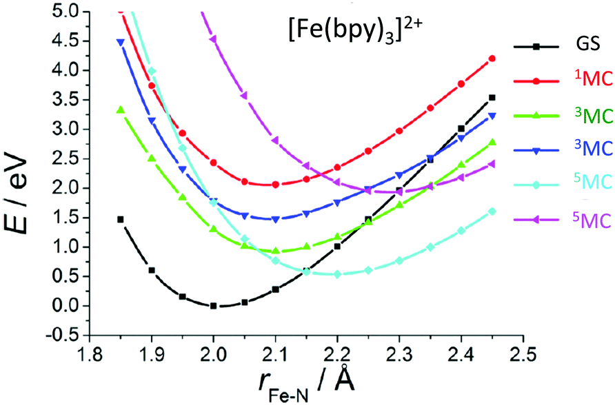
When studying in detail the theoretical results published on [Fe(bpy)3]2+![[thin space (1/6-em)]](https://www.rsc.org/images/entities/char_2009.gif) 81 for which the spin–vibronic coupling model has never been applied, we realized that we have here an ideal situation for ultrafast 1,3MLCT → 5MC decay (<100 fs) as compared to the NHC substituted molecules discussed above. Indeed, only the Fe–N stretching and bending modes are in play. Consequently, the early time vibrations affect less the MC states, excluding the opportunity for spawning conical intersections far away from the FC region as compared to the NHC substituted systems. In contrast, potentials associated with MLCT states may be slightly shifted in position and energy from the FC region, supporting an efficient 1,3MLCT → 1MC transition. Indeed, cuts of the calculated PES as a function of Fe–N bond stretching and calculated absorption spectra of [Fe(bpy)3]2+ at different levels (ab initio and TD-DFT)81 exhibit the presence of one 1MC state calculated at 2.61 eV (CASPT2) in the vicinity of the 1,3MLCT states calculated at 2.51 eV (CASPT2). In addition, a number of 3MC/5MC crossings coexist near the FC region (Fig. 3). We may expect ultrafast and efficient SOC driven vibronic assisted 1MLCT → 3MLCT and 1,3MLCT → 1,3MC transitions within a few tens of fs and population of the 5MC high-spin state as soon as the lowest 3MC state is populated. Further quantum dynamics simulations based on wavepacket propagations are needed to confirm the mechanism and put in evidence the role of the 1MC state.
81 for which the spin–vibronic coupling model has never been applied, we realized that we have here an ideal situation for ultrafast 1,3MLCT → 5MC decay (<100 fs) as compared to the NHC substituted molecules discussed above. Indeed, only the Fe–N stretching and bending modes are in play. Consequently, the early time vibrations affect less the MC states, excluding the opportunity for spawning conical intersections far away from the FC region as compared to the NHC substituted systems. In contrast, potentials associated with MLCT states may be slightly shifted in position and energy from the FC region, supporting an efficient 1,3MLCT → 1MC transition. Indeed, cuts of the calculated PES as a function of Fe–N bond stretching and calculated absorption spectra of [Fe(bpy)3]2+ at different levels (ab initio and TD-DFT)81 exhibit the presence of one 1MC state calculated at 2.61 eV (CASPT2) in the vicinity of the 1,3MLCT states calculated at 2.51 eV (CASPT2). In addition, a number of 3MC/5MC crossings coexist near the FC region (Fig. 3). We may expect ultrafast and efficient SOC driven vibronic assisted 1MLCT → 3MLCT and 1,3MLCT → 1,3MC transitions within a few tens of fs and population of the 5MC high-spin state as soon as the lowest 3MC state is populated. Further quantum dynamics simulations based on wavepacket propagations are needed to confirm the mechanism and put in evidence the role of the 1MC state.
 | ||
| Fig. 3 Cuts of the TD-DFT(B3LYP/TZP) calculated PES of [Fe(bpy)3]2+ as a function of Fe–N elongation (adapted from ref. 81a with permission from the American Chemical Society). | ||
The restricted number of normal modes included in the spin–vibronic Hamiltonian (up to five) and the accuracy of the electronic structure calculations are two limiting factors of fully quantum dynamics simulations that may bias the conclusions of the above studies dedicated to large transition metal complexes.
A recent work reported by Zobel et al.69c based on a LVC model coupled with TSH dedicated to [Fe(tpy)(pyz-NHC)]2+ (tpy = 2,2′:6′,2′-terpyridine;pyz-NHC = 1,1′-bis(2,6-diisopropylphenyl)pyrainyl-diimidazolium-2,2′-diylidene) illustrates the complexity of the analysis when increasing drastically the number of degrees of freedom in the simulation and the bias induced by reduced dimensionality. This study involving 20 singlet and 20 triplet electronic states, 244 normal modes, decoherence correction, SOC and solvent effects, while challenging, does not provide a sharp conclusion as far as the ultrafast dynamics is concerned in the absence of experimental data for this molecule. The manipulation of the LVC matrix by excluding some normal modes does not add clarity about the strong correlation between the electronic densities, tuning modes and intrastate coupling κ(n)i. The presence of one NHC ligand instead of two in [Fe(bmip)2]2+ and [Fe(btbip)2]2+ suggests that the Fe–C stretching modes will have less influence on the early time dynamics despite the presence of three 3MC states (2.56–2.76 eV) in the vicinity of the 1MLCT absorbing states (2.62–2.88 eV).
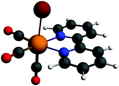
The two-step kinetics of ultrafast photolysis from a heme–CO complex (Fig. 4), namely τ < 50–70 fs attributed to the carbonyl loss and partial spin crossover and τ ∼300–400 fs ascribed to spin transition to high-spin states,82 has been investigated in detail using wavepacket quantum dynamics.52
 | ||
| Fig. 4 (a) Cartoon of the myoglobin active site. (b) Schematic structure of the heme–CO model complex. | ||
This complete quantum simulation includes 15 vibrational normal modes, and the low-lying 18 singlet, 20 triplet and 20 quintet electronic states coupled by SOC and vibronically up to the fifth order. The authors described an ultrafast CO release within 20 fs in the 1MLCT band prior to singlet to triplet transition estimated at 75 fs and triplet to quintet transition at 450 fs within a sequential mechanism. When scrutinizing the correlation between electronic densities, active normal modes and intrastate couplings in the heme–CO model complex used in the theoretical study, a more refined scenario can be proposed: after population of the Q band calculated at 2.73 eV, CO stretching (ν122 = 1478 cm−1), in-plane N-stretching (ν23 = 356 cm−1) and to a lesser extent out-of-plane porphyrin motion (ν26 =376 cm−1) (Fig. 5) generate large intrastate couplings in some specific excited states close to the Q band (Scheme 2).
 | ||
| Fig. 5 Major normal modes activated in the ultrafast CO photolysis in the heme-CO model complex (Fig. 4(b)) (adapted from ref. 52 with the permission of the authors). | ||

This leads to significant displacements of the potentials associated with the S41LMCT state calculated at 2.83 eV  with the T8 triplet mixed MLCT/MC/LLCT/LMCT state calculated at 2.56 eV
  and with the three lowest 1MC states
 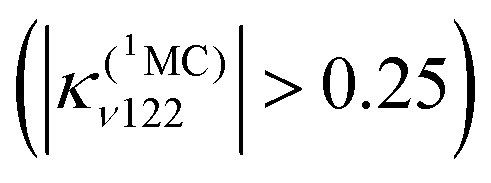 calculated between 1.90 eV and 2.36 eV.
Consequently, a negative shift in position and energy of these electronic states with respect to the initially populated Q state induces a number of conical intersections favouring their efficient and ultrafast population in the first few tens of fs, as illustrated by the diabatic population evolution shown in Fig. 6.
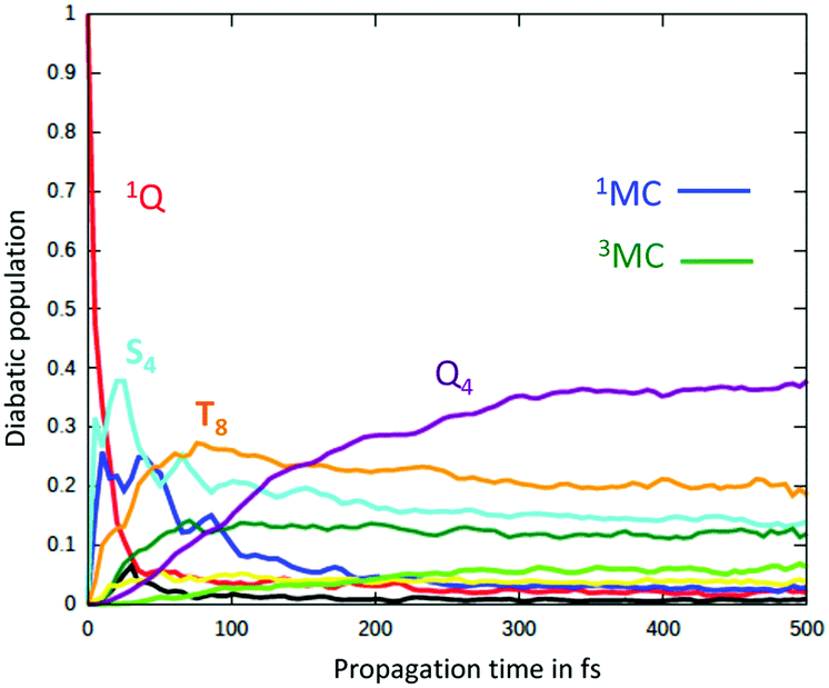 | ||
| Fig. 6 Time evolution of the diabatic population of the 1Q, S4, T8, 1MC and 3MC excited states of the heme–CO model complex (adapted from ref. 52 including SI with the permission of the authors). | ||
At the same time, Fe–CO stretching ν33 (Fig. 5) acts specifically on the pure 3MC states that involve Fe–CO bonding/antibonding orbitals, generating huge negative intrastate coupling  leading to drastic shifts of the associated potentials along this coordinate that drive their efficient population within about 70 fs (Fig. 6). These 3MC states certainly play a key role in the ultrafast dissociation of CO observed in the first few tens of fs, which cannot be solely attributed to the so-called 1MLCT band as proposed previously.52
Interestingly, the very close mode ν18, involving in addition to the Fe-out-of-plane CO dissociation the porphyrin ring motion (Fig. 5), acts similarly to ν33 on the lowest 3MC pure states but shifts the potentials in the opposite direction and less importantly. Moreover, these two modes generate large intrastate couplings of opposite signs in the quintet states as well  This certainly promotes triplet/quintet crossings that favour, together with SOC, efficient transition to the upper mixed MLCT/MC/LLCT/LMCT quintet state (Q4 calculated at 2.48 eV) within 100–150 fs (Fig. 6) and at longer time scales to the lowest 5MC states.
One of the most famous metal based photoswitches is the nitrosyl complex [RuCl(NO)(py)4]2+ (py = pyridine) depicted in Scheme 3.
 | ||
| Scheme 3 Schematic structure of [RuCl(NO)(py)4]2+. | ||
Its reversible high photoswitching ability has motivated a number of experimental84 and theoretical studies85 in the past ten years. Although the mechanism of NO photoisomerization (Fig. 7(a)) has been investigated using numerous static quantum chemical calculations, its nuclear dynamics has been recently studied for the first time.67c TSH including both non-adiabatic internal conversion and intersystem crossing has explored the early steps of the relaxation dynamics along different Ru–NO to Ru–ON pathways.
 | ||
| Fig. 7 (a) Mechanism of [RuCl(NO)(py)4]2+ photoisomerization based on DFT(B3LYP) and MS-CASPT2 calculations (adapted from ref. 87 with permission from the authors). (b) Three ultrafast decay pathways deduced from TSH dynamics.67c | ||
The difficulties here are twofold: (i) the electronic structure problem cannot be described consistently using density functional theory because the photoisomerization is a multiconfigurational problem; (ii) trajectory instabilities due to near-degeneracy of the electronic states cause collapses or divergences. Fortunately, previous ab initio calculations of the mechanism based on multiconfigurational methods provided a gauge for the reliability of TD-DFT results, especially the position of state crossings, for this specific complex potential energy surface landscape.
On the basis of highly accurate stationary MS-CASPT2 calculations and non-adiabatic TSH dynamic simulations in the gas phase, three mechanisms were proposed to coexist with a 3:2:4 branching ratio within the first 200 fs (Fig. 7(b)). The metastable isomer MS2 is accessible via two routes upon 1MLCT absorption at 473 nm, namely the triplet one combining fast ISC (∼200 fs) and internal conversion and the singlet one following the lowest singlet PES via several conical intersections. A third pathway, not envisioned by static calculations and involving an ultrafast ISC (80 fs), was evidenced by the non-adiabatic dynamics. Interestingly, the TSH non-adiabatic dynamics gives a nice picture of the electronic density evolution together with the Ru–N–O angle and Ru–NO bond length distribution as a function of time.
Simulation of the complete photo-isomerization pathway, until the formation of the metastable isomer MS1 (Fig. 7(a)), is beyond the current possibilities in terms of time-scale and trajectory stabilities. Although several approximations may be realistic for ultrafast photophysical processes, they are hardly applicable to complex photochemical mechanisms involving transition metal complexes.
3.2 Excited state dynamics in Cu(I) complexes
Early time-resolved spectroscopic and femtosecond fluorescence up-conversion experiments86 have shed new light on the photophysics of Cu(I)-phenanthroline complexes initially studied for their redox and luminescence properties in the 1980s87 as a competitor of [Ru(bpy)3]2+. [Cu(dmp)2]+ (dmp = 2,9-dimethyl-1,10-phenanthroline) (Scheme 4) and related complexes represent some of the best case studies in a number of misleading interpretations of the photophysics of transition metal complexes on the basis of the restrictive two-state (S1,T1) spin–orbit coupled model. | ||
| Scheme 4 Schematic structure of [Cu(dmp)2]+. | ||
As already pointed out by Zgierski in 200388 and discussed more recently within the context of TADF,89 Cu(I) complexes are characterized by closely low-lying triplet states near S1 and S2 that may participate in the photophysics, making the simple concept proposed for [Ru(bpy)3]2+ based on S1 → T1 (MLCT) ultrafast ISC invalid. Moreover, their excited state nuclear flexibility that provides their richness creates shallow minima and near-degeneracies on the low-lying PES requiring non-adiabatic quantum dynamics investigation based on accurate electronic structure data. By applying vibronic coupling Hamiltonian and wavepacket non-adiabatic dynamics to [Cu(dmp)2]+ within a fifteen “spin–orbit” states/eight normal modes model, including the pseudo-Jahn-Teller (PJT) coordinate, Capano et al.57c clarified the mechanism of ultrafast decay in the gas phase, putting an end to a long-standing controversy. A fast S3 → S2, S1 internal conversion (∼100 fs) occurs near the Franck–Condon region together with a flattening of the ligands activated by pseudo-JT distortion within 400 fs. This distortion creates S1/T2/T3 degeneracies favorable for efficient ISC within a sub-ps time-scale. The dominant normal modes are the symmetric Cu–N breathing mode ν8 calculated at 99 cm−1, which activates the initial S3 → S2, S1 transition, and the PJT rocking mode ν21 (b3) that couples strongly S1/S2 and T2/T3.57c
The kinetics associated with the pseudo-JT distortion (400 fs) and consequently the efficient occurrence of ISC depend drastically on the environment. A study combining TSH, wavepacket dynamics and QM/MM calculations16c argued that there was some influence of the solvent on the initial ultrafast decay within the singlet excited states. However, more recent studies dedicated to the early time structural dynamics of the lowest singlet states point to a nearly solvent independent fast component (∼100–200 fs) and to a slow component arising from the solvent/molecular vibration interplay within ∼1 ps.90 A detailed study in the gas phase by Du et al.91 evidenced the role of the assisting motion of the methyl substituents at the early stage of the dynamics together with an interligand flattening stabilized at ∼675 fs, in agreement with the most recent experiments.
The long story of Cu(I) complexes covering the last four decades clearly illustrates the necessity for an active and cooperative interplay between ultrafast time-resolved experiments and non-adiabatic dynamic simulations. This will be crucial to the success of potential applications in photovoltaic materials, OLEDs and TADF to name a few of them.
3.3 Ultrafast intersystem crossing in Re(I) complexes
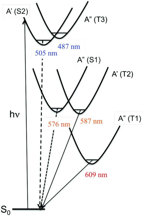
Rhenium(I) complexes are among the most investigated 3rd-row transition metal complexes, both experimentally and theoretically. This growing interest over the last two decades is due to their intriguing photophysical and photochemical properties that are able to generate specific functions in various environments, including large biological and macromolecular systems. These coordination compounds have been used as diagnostic and therapeutic tools, acting as luminescent and conformational probes92 or in light-triggered electron transfer processes.93 Rhenium(I) α-diimine carbonyls [Re(L)(CO)3(N,N)]n+ (L = halide, imidazole; N,N = bipyridine, phenanthroline) are thermally and photochemically robust and highly flexible synthetically. Structural variations of the N,N and L ligands have strong influences on the excited state properties of these chromophores. Visible light absorption provides the possibility of a wide range of applications such as sensors, probes, or emissive labels for bioimaging among others. One intriguing issue raised by the first time-resolved luminescence experiments94 is that the three energy domains and the three time domains reported are relatively constant within this class of molecules whatever the choice of the ligands and the solvent. Indeed, the 2D time-resolved luminescence spectra exhibit two luminescence signals at 500–550 nm and 550–600 nm associated with ultra-short time scales of 80 fs < τ1 < 150 fs and 0.3 ps < τ2 < 1.5 ps, respectively, and one signal below 610 nm with a phosphorescence time-scale varying from ns to ms, with only τ2 being slightly solvent dependent. The well accepted “cascade model” based on internal conversion (IC) vs. intersystem crossing (ISC) is unable to explain these experimental features. Early quantum dynamics simulations performed on this class of Re(I) complexes aimed at studying the role of structural dynamics in non-adiabatic ISC processes and at understanding why the “cascade model” breaks down.95 This work together with the quantum dynamics studies performed on Fe(II) and Cu(I) complexes described in the previous section shed new light on the spin–vibronic mechanism of ISC, establishing its importance in transition metal photophysics.42Another stimulating question has been raised by halide substituted complexes [Re(X)(CO)3(bpy)] (X = Cl, Br, or I; bpy = 2,2′-bipyridine), which exhibit complex electronic structure and large spin−orbit effects that do not correlate with heavy atom effects. Time-resolved luminescence experiments94 performed on this class of complexes have pointed to the role of structural dynamics in the kinetics of ISC. The 1MLCT → 3MLCT ISC kinetics in these 3rd-row compounds is slower than those in [Ru(bpy)3]2+ or [Fe(bpy)3]2+. Moreover, and counter intuitively, the expected heavy-atom effect within the series of halide-substituted complexes [Re(CO)3(bpy)] (X= Cl, Br, I) (Scheme 5), namely an increase of the ISC rate along the Cl, Br and I sequence, is not reproduced. Instead, the time scales of luminescence decays increase along the series with experimental values of τ1 = 85 ± 8 (Cl), 128 ± 12 (Br) and 152 ± 8 (I) fs, τ2 = 340 ± 50 (Cl), 470 ± 50 (Br) and 1180 ± 150 fs (I).94a Moreover, based on these experiments, a correlation has been proposed between the rhenium–halide stretch vibrational period and the kinetics of ISC (Fig. 8).
 | ||
| Scheme 5 Structure of the [Re(X)(CO)3(bpy)] complexes. | ||
 | ||
| Fig. 8 2D time-resolved luminescence spectrum of [Re(Cl)(CO)3(bpy)] in CH3CN (λexc = 400 nm) (a) and correlation of the ISC time-scales measured for [Re(X)(CO)3(bpy)] (X = Cl, Br, I) with the vibrational period of the Re–X stretching mode in similar complexes (adapted from ref. 94a with permission from the American Chemical Society). | ||
 | ||
| Scheme 6 Schematic representation of the potential energy curves associated with the low-lying excited states of [Re(Br)(CO)3(bpy)]. | ||
Static quantum chemical calculations based on TD-DFT calculations including solvent correction and SOC provide a clear qualitative picture of the photophysics of [Re(X)(CO)3(bpy)] controlled by the decay of two singlet (S1–S2) and three triplet (T1–T3) electronic excited states (Scheme 6).95b
The four lowest S1, S2, T1 and T2 photoactive electronic excited states of [Re(X)(CO)3(bpy)] are characterized by a mixed MLCT/XLCT (halide-to-ligand-charge-transfer) character, the composition of which depends significantly on the nature of the halide. In agreement with Raman experiments,96 the XLCT character of the S2/T2 and S1/T1 excited states increases with the heavy atom effect. T3 nearly degenerate with S2 corresponds to an intra-ligand (IL) excited state localized on the bpy.
Pioneering non-adiabatic quantum dynamics calculations performed on the bromide substituted complex [Re(Br)(CO)3(bpy)]95a,c evidenced the dominant normal modes able to activate significant vibronic couplings in this class of molecules. The normal mode activity is governed by symmetry rules (Cs symmetry in the present case), by absolute values of the generated coupling terms κ(n)i and λ(nm)i and by the character of the electronic excited state densities that correlate with the intrastate coupling term responsible for the shift in position and energy of the associated potential functions.95c,d For instance, ν9 and ν30 tuning modes associated with the CO vibrations (Fig. 9) activate rather large intrastate couplings in the MLCT/XLCT states and act differently on S1/T1 and S2/T2 (symmetry rules) with  and
and  generating conical intersections favorable to an efficient population of these electronic states. The key vibrational modes are the CO motions because of the metal-carbonyl bonding characteristics and the bpy vibrations, which act on the IL excited state (T3) and charge transfer electronic densities. The Re–X stretching mode ν11 acts similarly on the S1/T1 and S2/T2 excited state electronic densities (Fig. 9) with little impact on the potential shifts and generates rather small positive intrastate couplings in all states. The proposed correlation between the measured ISC time-scales and the Re–X vibration is fortuitous.
 | ||
| Fig. 9 Differences in electronic densities accompanying the S0 → S1/T1, S0 → S2/T2 and S0 → T3 transitions in [Re(Br)(CO)3(bpy)] (top) and some associated dominant symmetric tuning modes responsible for the intrastate coupling κ(n)i. | ||
A revealing illustration of the correlation between the vibrational activity, the electronic densities and the intrastate couplings was given by a recent study extended to the whole series of complexes [Re(X)(CO)3(bpy)] (X = F, Cl, Br, I).97 The non-adiabatic dynamics calculation of the complexes within 1.5 ps was performed using a multimode approach based on diabatic functions associated with S1, S2, T3, T2 and T1 giving rise to 11 “spin–orbit” electronic states and incorporating 14 normal modes (12a′ and 2a′′) within the quadratic vibronic coupling (QVC) model. The multiplet components were treated explicitly and SOC as well as the intra- and inter-state electron–vibration coupling terms was introduced into the W(Q) coupling matrix.
The time evolution of the diabatic population of the absorbing S2 excited state reveals an ultrafast exponential decay τ1 within a few tens of fs common to the four investigated complexes (Fig. 10). The early time theoretical decay of S2/T3 (in black in Fig. 10) coincides nearly perfectly with the experimental τ1 (in light blue in Fig. 10) extracted from a 3-parameter global fit for X = Cl and Br.94aτ1 was estimated at 93 ± 3 fs for X = Cl, comparable to the experimental value of 85 ± 8 fs.97
 | ||
| Fig. 10 Time-evolution of the population of the low-lying T3, S2/T2 and S1/T1 excited states in [Re(F)(CO)3(bpy)] (a), [Re(Cl)(CO)3(bpy)] (b) and [Re(Br)(CO)3(bpy)] (c). For the sake of clarity, the S2/T3 and S1/T2 populations are summed up.97 | ||
The simulations, including the one dedicated to the fluoride complex not investigated experimentally but predicted to decay within τ1 = 55 fs, reproduce rather well the trends within the series, namely an increase in the time scales within the halide series from the lighter to the heavier atom. The vibronic couplings induced by the carbonyl and bipyridine vibrations drive this ultra-fast decay, which is accompanied by population of the two intermediate states S1 and T2. The simulation performed on the iodide-substituted complex, not presented here, overestimates this effect with τ1 > 250 fs for an experimental value of ∼150 fs. This could be explained by the approach in perturbation used to describe the SOC effects that may amplify artificially the XLCT character in [Re(I)(CO)3(bpy)] leading to an underestimation of κ(n)i. The vibronic driven ultrafast decay of S2 is followed by the decay of the intermediate states S1 and T2 within a few hundreds of fs (τ2) and induced essentially by SOC with T1, the long-lived phosphorescent excited state. τ2 is estimated at 367± 31 fs vs. an experimental value of 340 ± 50 fs in [Re(Cl)(CO)3(bpy)].
The counterintuitive heavy atom effect observed experimentally is well reproduced by the quantum dynamics. Indeed, when increasing the XLCT character of the S1/T1 and S2/T2 electronic states within the series (Table 1), the tuning modes associated with the carbonyl vibrations induce a decrease of the κ(n)i intrastate couplings. As a consequence, perturbation of the diabatic potentials, namely shifts in position and in energy from the reference structure (Franck–Condon region), diminishes as well as the probability of occurrences of critical geometries favorable to efficient transfer of population from S2 to the intermediate states S1 and T2 and in fine to T1.
The mechanism of ultrafast ISC in [Re(X)(CO)3(bpy)] is stimulated by vibronic coupling and controlled by the XLCT electronic density contributions within the first 100 fs, with SOC being preeminent in the second step, namely the decay of the intermediate states and population of the long-lived T1 state. Remarkably, this mechanism differs from the one discovered for the imidazole substituted complex [Re(imidazole)(CO)3(phen)]+, which possesses pure MLCT states and an 3IL (T3) intermediate state efficiently populated within a few tens of fs. In this complex, the equilibration between T3 and T1 occurs within 70–80 fs and is observed both experimentally and in the quantum dynamics simulation. T3/T1 vibronic coupling controlled the transfer of population to T1. Interestingly, when the normal modes associated with the phenanthroline vibrations are frozen in the simulation, the T3 → T1 transition is quenched.95d,e
3.4 Other 3rd-row transition metal complexes
While excited state and photophysical properties of phosphorescent Ir(III) complexes have been extensively investigated because of their OLED potential, their early time dynamics is less explored. Following experimental studies98 dedicated to ultrafast ISC in [Ir(ppy)3] (ppy = 2-phenylpyridine), [Ir(ppy)2(bpy)] (bpy = 2,2′-bipyridine) and [Ir(ppz)2(dipy)] (ppz = 1-phenylpyrazole; dipy = 5-phenyldipyrrinato), Cui et al.99 studied the early time excited state non-adiabatic dynamics of the three complexes by means of a TD-DFT based mixed quantum-classical Generalized-TSH (G-TSH) method including 5 singlet and 10 triplet electronic states coupled by SOC. The simulations reproduce rather well the experimental trends, namely an increase in the ISC rate (65, 81 and 140 fs) along the [Ir(ppy)3], [Ir(ppy)2(bpy)], and [Ir(ppz)2(dipy)] series and the electronic properties of the ligands modulating the ultrafast Sn → Tn decay via ISC and IC processes. Combining their G-TSH method with QM/MM, the same authors investigated the ultrafast excited state relaxation in [Os(bpy)3] and [Os(bpy)2(dpp)] (dpp = 2,3-dipyridyl-pyrazine)100 that exhibit a rather significant inter-ligand-charge-transfer (ILCT) solvent dependence.101 The simulations show that ILCT plays a major role at the early stage of the relaxation dynamics.Finally, competition between the heavy atom effect and vibronic coupling in a series of donor–bridge–acceptor carbine metal–amide (metal = Cu, Ag, Au) emitter complexes was scrutinized by means of non-adiabatic quantum dynamics including SOC. This study points to the competition between direct ultrafast 1CT → 3CT ISC (Au; <100 fs) and population of an intermediate 3IL state populated within ∼65 fs in the Cu complex. The role of this intermediate state, largely stabilized when going from Au to Ag and Cu, becomes dominant in the Cu complex.102
4 Conclusion
The case studies presented in this perspective article illustrate with clarity why available quantum methods and current computational tools have to be used with care when dealing with ultrafast processes in transition metal complexes.Although the static picture based on stationary electronic structure properties (eigenstates, eigenenergies, and spin–orbit coupling) is correct for describing decays through “long-lived” S1 and T1 excited states following classical concepts developed in the 60s–70s for organic chromophores, this approach becomes inadequate for the interpretation of ultrafast relaxation processes within sub-ns time scales in coordination chemistry unless chemical and experimental environments can replicate “ideal” conditions. Indeed, the high density of states in a limited domain of energy, the variety of spin multiplicities, the nuclear flexibility, the degree of electronic mixing and the correlation between electronic densities and dominant normal modes generate crucial electron–vibration (vibronic) intrastate and inter-state couplings that control, together with SOC, the population in time of the individual excited states in the sub-ps regime. This opens a route to concurrent channels of deactivation, the interpretation of which is an experimental challenge.
For the further design of new coordination compounds with highly efficient functions applicable in various fields of chemistry and biology, one possibility is to tailor the photophysics chemically or environmentally to make the standard concepts pertinent for simple qualitative interpretation. The alternative is to modify our way of thinking complexity to obtain a correct interpretation and ultimately full control of the photophysics.
This complexity is even more dramatic when trying to properly include the environmental effects within the context of relaxation dynamics, another active field of research.103 The emergence of attoscience104 able to follow electron molecular dynamics in complex systems105 has opened a new domain dedicated to the correlated motion of electrons and nuclei in the attosecond (as) time scale,106 revealing a ground-breaking picture of molecular quantum properties with fundamental issues that remain to be discovered.
Conflicts of interest
There are no conflicts to declare.References
- M. K. DeArmond, Acc. Chem. Res., 1974, 7, 309–315 CrossRef CAS.
- K. W. Hipps, G. A. Merrell and G. A. Crosby, J. Phys. Chem., 1976, 80, 2232–2239 CrossRef CAS; D. R. Striplin and G. A. Crosby, Chem. Phys. Lett., 1994, 221, 426–430 CrossRef; D. R. Striplin and G. A. Crosby, J. Phys. Chem., 1995, 99, 7977–7984 CrossRef; A. F. Rausch, M. E. Thompson and H. Yersin, Inorg. Chem., 2009, 48, 1928–1937 CrossRef; A. F. Rausch, M. E. Thompson and H. Yersin, J. Phys. Chem. A, 2009, 113, 5927–5932 CrossRef; A. Bossi, A. F. Rausch, M. J. Leitl, R. Czerwieniec, M. T. Whited, P. I. Djurovich, H. Yersin and M. E. Thompson, Inorg. Chem., 2013, 52, 12403–12415 CrossRef.
- J. Z. Zhao, S. M. Ji, W. H. Wu, W. T. Wu, H. M. Guo, J. F. Sun, H. Y. Sun, Y. F. Liu, Q. T. Li and L. Huang, RSC Adv., 2012, 2, 1712–1728 RSC.
- J. Z. Zhao, K. J. Xu, W. B. Yang, Z. J. Wang and F. F. Zhong, Chem. Soc. Rev., 2015, 44, 8904–8939 RSC.
- B. K. T. Batagoda, P. I. Djurovich, S. Brase and M. E. Thompson, Polyhedron, 2016, 116, 182–188 CrossRef CAS; W. Wei, S. A. M. Lima, P. I. Djurovich, A. Bossi, M. T. Whited and M. E. Thompson, Polyhedron, 2018, 140, 138–145 CrossRef.
- Y. Xu, J. Wang, W. Zhang, W. Li and W. Shen, J. Photochem. Photobiol., A, 2017, 346, 225–235 CrossRef CAS.
- Photophysics of Organometallics, ed. A. J. Lee, Topics in Organometallic Chemistry, Springer-Verlag, Berlin-Heidelberg, 2010, vol. 29, pp. 1–237 CrossRef CAS; G. Baryshnikov, B. Minaev and H. Agren, Chem. Rev., 2017, 117, 6500–6537 CrossRef CAS.
- H. Yersin and J. Strasser, Coord. Chem. Rev., 2000, 208, 331–364 CrossRef CAS; H. Hofbeck and H. Yersin, Inorg. Chem., 2010, 49, 9290–9299 CrossRef; H. Yersin, A. F. Rausch, R. Czerwieniec, T. Hofbeck and T. Fischer, Coord. Chem. Rev., 2011, 255, 2622–2652 CrossRef; R. Czerwieniec, M. J. Leitl, H. H. H. Homeier and H. Yersin, Coord. Chem. Rev., 2016, 325, 2–28 CrossRef.
- Photochemistry and Photophysics of Coordination Compounds Top. in Curr. Chem., ed. V. Balzani and S. Campagna, 2007, vol. 280, Springer-Verlag, Berlin-Heidelberg CrossRef CAS; Photophysics of Organometallics Top. in Curr. Chem., ed. A. J. Lees, Springer-Verlag, Berlin-Heidelberg, 2010, vol 29 CrossRef CAS; F. N. Castellano, Acc. Chem. Res., 2015, 48, 828–839 CrossRef CAS; K. K.-W. Lo, Acc. Chem. Res., 2015, 48, 2985–2995 CrossRef; K. Y. Zhang, Q. Yu, H. J. Wei, S. J. Liu, Q. Zhao and W. Huang, Chem. Rev., 2018, 118, 1770–18390 CrossRef.
- M. Chergui, Acc. Chem. Res., 2015, 48, 801–808 CrossRef CAS; A. Vlček Jr, Coord. Chem. Rev., 2000, 200/202, 933–977 CrossRef; M. Chergui, Dalton Trans., 2012, 41, 13022–13029 RSC.
- S. Straub, L. I. Domenianni, J. Lindner and P. Vöhringer, J. Phys. Chem. B, 2019, 123, 7893–7904 CrossRef CAS.
- H. Song, X. Wang, W. W. Yang, G. He, Z. Kuang, Y. Li, A. Xia, Y.-W. Zhong and F. Kong, Chem. Phys. Lett., 2017, 683, 322–328 CrossRef CAS; A. M. Brown, C. E. McCusker, M. C. Carey, A. M. Blanco-Rodríguez, M. Towrie, I. P. Clark, A. Vlček and J. K. McCusker, J. Phys. Chem. A, 2018, 122, 7941–7953 CrossRef; M. C. Carey, S. L. Adelman and J. K. McCusker, Chem. Sci., 2019, 10, 134–144 RSC; I. V. Sazanovich, J. Best, P. A. Scattergood, M. Towrie, S. A. Tikhomirov, O. V. Bouganov, A. J. H. M. Meijer and J. A. Weinstein, Phys. Chem. Chem. Phys., 2014, 16, 25775–25788 RSC; P. A. Scattergood, M. Delor, I. V. Sazanovich, O. V. Bouganov, S. A. Tikhomirov, A. S. Stasheuski, A. W. Parker, G. M. Greetham, M. Towrie, E. S. Davies, A. J. H. M. Meije and J. A. Weinstein, Dalton Trans., 2014, 43, 17677–17693 RSC; P. A. Scattergood, M. Delor, I. V. Sazanovich, M. Towrie and J. A. Weinstein, Faraday Discuss., 2015, 185, 69–86 RSC.
- P. Kim, M. S. Kelley, A. Chakraborty, N. L. Wong, R. P. Van Duyne, G. C. Schatz, F. N. Castellano and L. X. Chen, J. Phys. Chem. C, 2018, 122, 14195–14204 CrossRef CAS.
- K. Kunnus, M. Vacher, T. C. B. Harlang, K. S. Kjær, K. Haldrup, E. Biasin, T. B. van Driel, M. Pápai, P. Chabera, Y. Liu, H. Tatsuno, C. Timm, E. Källman, M. Delcey, R. W. Hartsock, M. E. Reinhard, S. Koroidov, M. G. Laursen, F. B. Hansen, P. Vester, M. Christensen, L. Sandberg, Z. Németh, D. S. Szemes, E. Bajnóczi, R. Alonso-Mori, J. M. Glownia, S. Nelson, M. Sikorski, D. Sokaras, H. T. Lemke, S. E. Canton, K. B. Møller, M. M. Nielsen, G. Vankó, K. Wärnmark, V. Sundström, P. Persson, M. Lundberg, J. Uhlig and K. J. Gaffney, Nat. Commun., 2020, 11, 634–644 CrossRef CAS.
- M. Iwamura, K. Kimoto, K. Nozaki, H. Kuramochi, S. Takeuchi and T. Tahara, J. Phys. Chem. Lett., 2018, 9, 7085–7089 CrossRef CAS.
- (a) M. Iwamura, H. Watanabe, K. Ishii, S. Takeuchi and T. Tahara, J. Am. Chem. Soc., 2011, 133, 7728–7736 CrossRef CAS; (b) L. Hua, M. Iwamura, S. Takeuchi and T. Tahara, Phys. Chem. Chem. Phys., 2015, 17, 2067–2077 RSC; (c) G. Capano, T. J. Penfold, M. Chergui and I. Tavernelli, Phys. Chem. Chem. Phys., 2017, 19, 19590–19600 RSC; (d) L. Shen, T.-F. He, L.-Y. Zou, J.-F. Guo and A.-M. Ren, Org. Electron., 2020, 81, 105664–1056674 CrossRef CAS; (e) G. Levi, E. Biasin, A. O. Dohn and H. Jonsson, Phys. Chem. Chem. Phys., 2020, 22, 748–757 RSC.
- M. Delor, P. A. Scattergood, I. V. Sazanovich, A. W. Parker, G. M. Greetham, A. J. H. M. Meijer, M. Towrie and J. A. Weinstein, Science, 2014, 346, 1492–1494 CrossRef CAS; M. Delor, T. Keane, P. A. Scattergood1, I. V. Sazanovich, G. M. Greetham, M. Towrie, A. J. H. M. Meijer and J. A. Weinstein, Nat. Chem., 2015, 7, 689–695 CrossRef; M. Delor1, S. A. Archer, T. Kean, A. J. H. M. Meijer1, I. V. Sazanovich, G. M. Greetham, M. Towrie and J. A. Weinstein, Nat. Chem., 2017, 9, 1099–1104 CrossRef.
- Time-Dependent Density Functional Theory, ed. M. A. L. Marques, C. A. Ullrich, F. Nogueira, A. Rubio, K. Burke and E. K. U. Gross, Springer-Verlag, 2006, ISBN 978-3-540-35422-2 CrossRef CAS; M. E. Casida, Theoretical and Computational Chemistry, Elsevier, New York, 1996, vol. 4, pp. 391–439 CrossRef CAS; M. E. Casida, C. Jamorski, K. C. Casida and D. R. Salahub, J. Chem. Phys., 1998, 108, 4439 CrossRef CAS; R. E. Stratmann, G. E. Scuseria and M. J. Frisch, J. Chem. Phys., 1998, 109, 8218 CrossRef; S. Hirata and M. Head-Gordon, Chem. Phys. Lett., 1999, 302, 375 CrossRef.
- C. D. Sherrill and H. F. Schaefer III, in The Configuration Interaction Method: Advances in Highly Correlated Approaches. Advances in Quantum Chemistry. ed. P.-O. Löwdin, San Diego, Academic Press, 1999, vol. 34, pp. 143–269 Search PubMed.
- B. O. Roos, The Multiconfigurational (MC) Self-Consistent Field (SCF) Theory. in Lecture Notes in Quantum Chemistry. Lecture Notes in Chemistry, ed. B. O. Roos, Springer, Berlin, Heidelberg, vol. 58, 1992 Search PubMed.
- B. O. Roos, P. R. Taylor and P. E. M. Siegbahn, Chem. Phys., 1980, 48, 157–173 CrossRef CAS.
- K. Andersson, P.-Å. Malmqvist, B. O. Roos, A. Sadlej and K. Wolinski, J. Phys. Chem., 1990, 94, 5483–5486 CrossRef CAS; K. Andersson, P.-Å. Malmqvist and B. O. Roos, J. Chem. Phys., 1992, 96, 1218–1226 CrossRef.
- M. Turki, C. Daniel, S. Záliš, A. Vlček, J. van Slageren and D. J. Stufkens, J. Am. Chem. Soc., 2001, 123(46), 11431–11440 CrossRef CAS.
- M. Fumanal and C. Daniel, J. Comput. Chem., 2016, 37, 2454–2466 CrossRef CAS.
- J. Olsen, B. O. Roos, P. Jörgensen and H. J. A. Jensen, J. Chem. Phys., 1988, 89, 2185–2192 CrossRef CAS.
- D. Ma, G. Li Manni and L. Gagliardi, J. Chem. Phys., 2011, 135, 044128 CrossRef.
- G. Li Manni, F. Aquilante and L. Gagliardi, J. Chem. Phys., 2011, 134, 034114 CrossRef.
- M. R. Hermes and L. Gagliardi, J. Chem. Theory Comput., 2019, 15, 972–986 CrossRef CAS; R. Pandharkar, M. R. Hermes, C. J. Cramer and L. Gagliardi, J. Phys. Chem. Lett., 2019, 10, 5507–5513 CrossRef.
- J. Ivanic, J. Chem. Phys., 2003, 119, 9364–9376 CrossRef CAS.
- R. Pandharkar, M. R. Hermes, C. J. Cramer and L. Gagliardi, J. Phys. Chem. Lett., 2019, 10, 5507–5513 CrossRef CAS.
- M. Joani and M. S. Gordon, Phys. Chem. Chem. Phys., 2018, 20, 2615–2626 RSC; M. Joani and M. S. Gordon, J. Phys. Chem. A, 2019, 123, 1260–1272 CrossRef; M. Joani and M. S. Gordon, Phys. Chem. Chem. Phys., 2020, 22, 1475–1484 RSC.
- K. H. Marti and M. Reiher, Phys. Chem. Chem. Phys., 2011, 13, 6750–6759 RSC; S. Sharma and G. K.-L. Chan, J. Chem. Phys., 2012, 136, 124121 CrossRef CAS.
- C. J. Stein and M. Reiher, J. Chem. Theory Comput., 2016, 12, 1760–1771 CrossRef CAS; C. J. Stein and M. Reiher, J. Comput. Chem., 2019, 40, 2216–2226 Search PubMed.
- Q. M. Phung, S. Wouters and K. Pierloot, J. Chem. Theory Comput., 2016, 12, 4352–4361 CrossRef CAS; Q. M. Phung and K. Pierloot, J. Chem. Theory Comput., 2019, 15, 3033–3043 CrossRef; M. A. Reiher, Chimia, 2009, 63, 140–145 CrossRef.
- N. Mardirossian and M. Head-Gordon, Mol. Phys., 2017, 115, 2315–2372 CrossRef CAS.
- C. Daniel, Density Functional Theories and Coordination Chemistry, Reference Module in Chemistry, Molecular Sciences and Chemical Engineering, Elsevier, 2020, ISBN 9780124095472 DOI:10.1016/B978-0-12-409547-2.14828-0.
- L. Gagliardi, D. G. Truhlar, G. Li Manni, R. K. Carlson, C. E. Hoyer and J. W. L. Bao, Acc. Chem. Res., 2017, 50, 66–73 CrossRef CAS.
- A. Heil, M. Kleinschmidt and C. M. Marian, J. Chem. Phys., 2018, 149, 64106 CrossRef; C. M. Marian, A. Heil and M. Kleinschmidt, Wiley Interdiscip. Rev.: Comput. Mol. Sci., 2019, 9, E1394 Search PubMed.
- Density Functional Theory for Excited States, Topics in Current Chemistry, ed. N. Ferré, M. Filatov and M. Huix Rotllant, Springer, Berlin, 2016, vol. 368 Search PubMed; C. Daniel, Density Functional Theories and Coordination Chemistry, Reference Module in Chemistry, Molecular Sciences and Chemical Engineering, Elsevier, 2020, ISBN 9780124095472 DOI:10.1016/B978-0-12-409547-2.14828-0.
- C. Daniel, Coord. Chem. Rev., 2015, 282–283, 19–32 CrossRef CAS; S. Xu, J. E. T. Smith, S. Gozem, A. I. Krylov and J. M. Weber, Inorg. Chem., 2017, 56, 7029–7037 CrossRef; K. Falahati, C. Hamerla, M. Huix-Rotllant and I. Burghardt, Phys. Chem. Chem. Phys., 2018, 20, 12483–12492 RSC.
- H. Köppel, W. Domcke and L. S. Cederbaum, Adv. Chem. Phys., 1984, 57, 59–246 Search PubMed.
- T. J. Penfold, E. Gindensperger, C. Daniel and C. M. Marian, Chem. Rev., 2018, 118, 6975–7625 CrossRef CAS.
- D. C. Ashley and E. Jakubikova, Coord. Chem. Rev., 2017, 337, 97–111 CrossRef CAS; C. Daniel, Density Functional Methods for Excited States Book series: Topics in Current Chemistry, 2016, 368, 377–413 Search PubMed; N. M. S. Almeida, R. G. McKinlay and M. J. Paterson, in Computation of Excited States of Transition Metal Complexes. ed. Macgregor S. and Eisenstein O., Computational Studies in Organometallic Chemistry; Structure and Bonding, Springer, Cham, 2014, vol. 167 Search PubMed.
- L. Lang and F. Neese, J. Chem. Phys., 2019, 150, 10414 CrossRef CAS; F. Neese, J. Am. Chem. Soc., 2006, 128, 10213–10222 CrossRef; F. Neese, T. Petrenko, D. Ganyushin and G. Olbrich, Coord. Chem. Rev., 2007, 251, 288–327 CrossRef; C. Duboc, D. Ganyushin, K. Sivalingam, K. M.-N. Collomb and F. Neese, J. Phys. Chem. A, 2010, 114, 10750–10758 CrossRef.
- E. van Lenthe, A. E. Ehlers and E. J. Baerends, J. Chem. Phys., 1999, 110, 8943 CrossRef CAS.
- B. de Souza, F. Giliandro, F. Neese and R. Izsák, J. Chem. Theory Comput., 2019, 15, 1896–1904 CrossRef CAS.
- P.-Å. Malmqvist, B. O. Roos and B. Schimmelpfennig, Chem. Phys. Lett., 2002, 357, 230–240 CrossRef CAS.
- B. A. Heß, C. M. Marian, U. Wahlgren and O. Gropen, Chem. Phys. Lett., 1996, 251, 365–371 CrossRef.
- C. M. Marian, Wiley Interdiscip. Rev.: Comput. Mol. Sci., 2012, 2, 187–203 CAS.
- F. Plasser, M. Ruckenbauer, S. Mai, M. Oppel, P. Marquetand and L. Gonzalez, J. Chem. Theory Comput., 2016, 12, 1207–1219 CrossRef CAS.
- M. Fumanal, F. Plasser, S. Mai, C. Daniel and E. Gindensperger, J. Chem. Phys., 2018, 148, 124119 CrossRef.
- K. Falahati, H. Tamura, I. Burghardt and M. Huix-Rotlant, Nat. Commun., 2018, 9, 4502 CrossRef.
- N. Balakrishnan, C. Kalyanaraman and N. Sathymurthy, Phys. Rep., 1997, 280, 79–144 CrossRef CAS; G. G. Balint-Kurti, R. N. Dixon and C. C. Marston, Int. Rev. Phys. Chem., 1992, 11(2), 317–344 Search PubMed; H.-D. Meyer, F. Gatti, G. A. Worth, Multidimensional Quantum Dynamics, Wiley-VCH, Weinheim, 2009 Search PubMed.
- H. Beck, A. Jäckle, G. A. Worth and H.-D. Meyer, Phys. Rep., 2000, 324(1), 1 CrossRef.
- U. Manthe, J. Chem. Phys., 2008, 128, 164116 CrossRef.
- M. Fumanal, E. Gindensperger and C. Daniel, J. Chem. Theory Comput., 2017, 13, 1293–1306 CrossRef CAS; M. Fumanal, E. Gindensper and C. Daniel, Phys. Chem. Chem. Phys., 2018, 20, 1134–1141 RSC; Y. Harabuchi, J. Eng, E. Gindensperger, T. Taketsugu, S. Maeda and C. Daniel, J. Chem. Theory Comput., 2016, 12, 2335–2345 CrossRef; J. Eng, C. Gourlaouen, E. Gindensperger and C. Daniel, Acc. Chem. Res., 2015, 48, 809–817 CrossRef.
- (a) M. Fumanal, E. Gindensperger and C. Daniel, J. Phys. Chem. Lett., 2018, 9, 5189–5195 CrossRef CAS; (b) M. Pápai, G. Vankó, T. Rozgonyi and T. J. Penfold, J. Phys. Chem. Lett., 2016, 7, 2009–2014 CrossRef; (c) G. Capano, M. Chergui, U. Rothlisberger, I. Tavernelli and T. J. Penfold, J. Phys. Chem. A, 2014, 118, 9861–9869 CrossRef CAS; (d) M. Pápai, T. Rozgonyi, T. J. Penfold, M. N. Nielsen and K. B. Moller, J. Chem. Phys., 2019, 151, 104307 CrossRef.
- I. Burghardt, H.-D. Meyer and L. S. Cederbaum, J. Chem. Phys., 1999, 111, 2927–2939 CrossRef CAS.
- G. A. Worth, M. Robb and I. Burghardt, Faraday Discuss., 2004, 127, 307–323 RSC; B. Lasorne, G. A. Worth and M. A. Robb, Wiley Interdiscip. Rev.: Comput. Mol. Sci., 2011, 1, 460–475 Search PubMed.
- G. Richings, I. Polyak, K. Spinlove, G. Worth, I. Burghardt and B. Lasorne, Int. Rev. Phys. Chem., 2015, 34, 269–308 Search PubMed.
- D. V. Shalashilin, J. Chem. Phys., 2009, 130, 244101 CrossRef.
- M. Ben-Nun, J. Quenneville and T. J. Martinez, J. Phys. Chem. A, 2000, 104, 5161–5175 CrossRef CAS.
- D. V. Makhov, W. J. Glower, T. J. Martinez and D. V. Shalashilin, J. Chem. Phys., 2014, 141, 054110 CrossRef.
- A. Bera, J. Ghosh and A. Bhattacharya, J. Chem. Phys., 2017, 147, 044308 CrossRef.
- J. C. Tully, Chem. Phys., 1990, 93, 1061–1071 CAS.
- S. Mai, P. Marquetand and L. Gonzalez, Wiley Interdiscip. Rev.: Comput. Mol. Sci., 2018, 8, e1370 Search PubMed.
- (a) A. J. Atkins and L. Gonzalez, J. Phys. Chem. Lett., 2017, 8, 3840–3845 CrossRef CAS; (b) S. Mai and L. Gonzalez, Chem. Sci., 2019, 10, 10405–10411 RSC; (c) F. Talotta, M. Boggio-Pasqua and L. Gonzalez, Chem. – Eur. J., 2020, 26, 11522–11528 CrossRef CAS; (d) S. Mai, M. F. S. J. Menger, M. Marazzi, D. L. Stolba, A. Monari and L. Gonzalez, Theor. Chem. Acc., 2020, 139, 65 Search PubMed.
- F. Plasser, S. Gomez, M. F. S. J. Menger, S. Mai and L. Gonzalez, Phys. Chem. Chem. Phys., 2019, 21, 57–69 RSC.
- (a) F. Plasser, S. Mai, M. Fumanal, E. Gindensperger, C. Daniel and L. Gonzalez, J. Chem. Theory Comput., 2019, 15, 5031–5045 CrossRef CAS; (b) S. Mai and L. Gonzalez, J. Chem. Phys., 2019, 151, 244115-1-14 CrossRef; (c) J. P. Zobel, O. S. Bokareva, P. Zimmer, C. Wölper, M. Bauer and L. Gonzalez, Inorg. Chem., 2020, 59, 14666–14678 CrossRef CAS.
- S. K. Min, F. Agostini and E. K. U. Gross, Phys. Rev. Lett., 2015, 115, 073001 CrossRef CAS; F. Agostini, S. K. Min, A. Abedi and E. K. U. Gross, J. Chem. Theory Comput., 2016, 12, 2127–2143 CrossRef; J.-K. Ha, I. S. Lee and S. K. Min, J. Phys. Chem. Lett., 2018, 9, 1097–1104 CrossRef.
- S. K. Min, F. Agostini, I. Tavernelli and E. K. U. Gross, J. Phys. Chem. Lett., 2017, 8, 3048–3055 CrossRef CAS.
- F. Agostini and B. F. E. Curchod, Wiley Interdiscip. Rev.: Comput. Mol. Sci., 2019, 9, E1417 Search PubMed.
- S. Decurtins, P. Guthlich, C. Kohler, H. Spiering and A. Hauser, Chem. Phys. Lett., 1984, 105, 1–4 CrossRef CAS; A. Hauser, A. Vef and P. Adler, J. Chem. Phys., 1991, 95, 8710 CrossRef.
- O. Bräm, F. Messina, A. M. El-Zohry, A. Cannizzo and M. Chergui, Chem. Phys., 2012, 393, 51–57 CrossRef CAS; A. Cannizzo, F. van Mourik, W. Gawelda, G. Zgrablic, C. Bressler and M. Chergui, Angew. Chem., 2006, 118, 3246–3248 CrossRef; N. H. Damrauer, G. Cerullo, A. Yeh, T. R. Boussie, C. V. Shank and J. K. McCusker, Science, 1997, 275, 54–57 CrossRef; A. T. Yeh, C. V. Shank and J. K. McCusker, Science, 2000, 289, 935–938 CrossRef; A. Cannizzo, C. J. Milne, C. Consani, W. Gawelda, C. Bressler, F. van Mourik and M. Chergui, Coord. Chem. Rev., 2010, 254, 2677–2686 CrossRef; W. Zhang, et al. , Nature, 2014, 509, 345–348 CrossRef; G. AuBöck and M. Chergui, Nature, 2015, 7, 629–633 Search PubMed.
- Y. Liu, T. C. Harlang, S. E. Canton, P. Chabera, K. Suarez-Alcantara, A. Fleckhaus, D. A. Vithanage, E. Göransson, A. Corani, R. Lomoth, V. Sundström and K. Wärnmark, Chem. Commun., 2013, 57, 6412–6414 RSC.
- P. Chabera, K. S. Kjaer, O. Prakash, A. Honarfar, Y. Liu, L. A. Fredin, T. C. Harlang, S. Lidin, J. Uhlig, V. Sundström, R. Lomoth, P. Persson and K. Wärnmark, J. Phys. Chem. Lett., 2018, 9, 459–463 CrossRef CAS; K. S. Kjaer, et al. , Science, 2019, 363, 249–253 CrossRef.
- L. A. Fredin, M. Papai, E. Rozsalyi, G. Vanko, K. Wärnmark, V. Sundström and P. Persson, J. Phys. Chem. Lett., 2014, 5, 2066–2071 CrossRef CAS.
- M. Papai, T. J. Penfold and K. B. Moller, J. Phys. Chem. C, 2016, 120, 17234–17241 CrossRef CAS.
- M. Papai, M. Simmermacher, T. J. Penfold and K. B. Moller, J. Chem. Theory Comput., 2018, 14, 3967–3974 CrossRef CAS.
- M. Papai, M. Abedi, G. Levi, E. Biasin, M. M. Nielsen and K. B. Moller, J. Phys. Chem. C, 2019, 123, 2056–2065 CrossRef CAS.
- (a) M. Papai, G. Vanko, C. de Graaf and T. Rozgonyi, J. Chem. Theory Comput., 2013, 9, 509–519 CrossRef CAS; (b) C. Sousa, C. de Graaf, A. Rudavskyi, R. Broer, J. Tatchen, M. Etinski and C. M. Marian, Chem. – Eur. J., 2013, 19, 17541–17551 CrossRef CAS.
- M. Levantino, G. Schiro, H. T. Lemke and G. Cottone, Laser Nat. Commun., 2015, 6, 6772 CrossRef CAS; M. Levantino, et al. , Struct. Dyn., 2015, 2, 041713 CrossRef; S. Franzen, L. Kiger, C. Poyart and J. L. Martin, Biophys. J., 2001, 80, 2372–2385 CrossRef.
- I. Tavernelli, B. F. E. Curchod and U. Rothlisberger, Chem. Phys., 2011, 391, 101–109 CrossRef CAS.
- D. Schaniel, B. Cormary, I. Malfant, V. Lydie, V. Theo, V. Bernard, K. V. Kramer and H.-U. Gudel, Phys. Chem. Chem. Phys., 2007, 9, 3717–3724 RSC; B. Cormary, I. Malfant, L. Valade, M. Buron-Le-Cointe, L. Toupet, T. Todorova, B. Delley, D. Schaniel, N. Mockus, T. Voike, K. Fejfarova, V. Petricek and M. Dusek, Acta Crystallogr., Sect. B: Struct. Sci., Cryst. Eng. Mater., 2009, 65, 787 CrossRef CAS; B. Cormary, S. Ladeira, K. Jacob, P. G. Lacroix, T. Voike, D. Schaniel and I. Malfant, Inorg. Chem., 2012, 51, 7492–7501 CrossRef; A. G. De Candia, J. P. Marcolongo, R. Etchenique and L. D. Slep, Inorg. Chem., 2010, 49, 6925–6930 CrossRef.
- J. Sanz Garcia, F. Alary, M. Boggio-Pasqua, I. M. Dixon, I. Malfant and J.-L. Heully, Inorg. Chem., 2015, 54, 8310–8318 CrossRef CAS; J. Sanz Garcia, F. Alary, M. Boggio-Pasqua, I. M. Dixon and J.-L. Heully, J. Mol. Model., 2016, 22, 284 CrossRef; F. Talotta, J.-L. Heully, F. Alary, I. M. Dixon, L. Gonzalez and M. Boggio-Pasqua, J. Chem. Theory Comput., 2017, 13, 6120–6130 CrossRef.
- L. X. Chen, G. Shaw, I. Novozhilova, T. Liu, G. Jennings, K. Attenkofer, G. Meyer and P. Coppens, J. Am. Chem. Soc., 2003, 125, 7022–7034 CrossRef CAS; M. Iwamura, S. Takeuchi and T. Tahara, J. Am. Chem. Soc., 2007, 129, 5248–5256 CrossRef; G. B. Shaw, C. D. Grant, H. Shirota, E. W. Castner, G. J. Meyer and L. X. Chen, J. Am. Chem. Soc., 2007, 129, 2147–2160 CrossRef.
- M. W. Blaskie and D. R. McMillin, Inorg. Chem., 1980, 19, 3519–3522 CrossRef CAS; C. O. Dietrich-Buchecker, P. A. Marnot, J.-P. Sauvage, J. R. Kirchhoff and D. R. McMillin, J. Chem. Soc., Chem. Commun., 1983, 513–515 RSC; D. G. Cuttel, S.-M. Kuang, P. E. Fanwick, D. R. McMillin and R. A. Walton, J. Am. Chem. Soc., 2002, 124(1), 6–7 CrossRef; N. Armaroli, G. Accorsi, F. Cardinali and A. Listorti, Top. Curr. Chem., 2007, 280, 69–115 CrossRef Springer-Verlag Berlin Heidelberg.
- M. Zgierski, J. Chem. Phys., 2003, 118, 4045 CrossRef CAS.
- A. Stoianov, C. Gourlaouen, S. Vela and C. Daniel, J. Phys. Chem. A, 2018, 122, 1413–1421 CrossRef CAS.
- G. Levi, E. Biasin, A. O. Dohn and H. Jonsson, Phys. Chem. Chem. Phys., 2020, 22, 748–757 RSC.
- L. Du and Z. Lan, Phys. Chem. Chem. Phys., 2016, 18, 7641–7650 RSC.
- K. K. W. Lo, Acc. Chem. Res., 2020, 53, 32–44 CrossRef CAS; E. B. Bauer, A. A. Haase, R. M. Reich, D. C. Crans and F. E. Kühn, Coord. Chem. Rev., 2019, 393, 79–117 CrossRef; L. K. McKenzie, H. E. Bryant and J. A. Weinstein, Coord. Chem. Rev., 2019, 379, 2–29 CrossRef; A. M.-H. Yip and K. K. W. Lo, Coord. Chem. Rev., 2018, 361, 138–163 CrossRef; L. C. C. Lee, K.-K. Leung and K. K. W. Lo, Dalton Trans., 2017, 46, 16357–16380 RSC.
- J. J. Warren, M. E. Ener, A. Vlcek Jr, J. R. Winkler and H. B. Gray, Coord. Chem. Rev., 2012, 256, 2478–2487 CrossRef CAS; C. Shih, A. K. Museth, M. A. Brahamsson, A. M. Blanco-Rodriguez, A. J. Di Bilio, J. Sudhamsu, B. B. Crane, K. L. Ronayne, M. Towrie, A. Vlcek Jr., J. H. Richards, J. R. Winkle and H. B. Gray, Science, 2008, 320, 1760–1762 CrossRef; A. M. Blanco-Rodriguez, M. Busby, C. Gradinaru, B. R. Crane, A. J. Di Bilio, P. Matousek, M. Towrie, B. S. Leigh, J. H. Richards, A. Vlcek, Jr. and H. B. Gray, J. Am. Chem. Soc., 2006, 128, 4365–4370 CrossRef; A. J. Di Bilio, B. R. Crane, W. A. Wehbi, C. N. Kiser, M. M. Abu-Omar, R. M. Carlos, J. H. Richards, J. R. Winkler and H. B. Gray, J. Am. Chem. Soc., 2001, 123, 3181–3182 CrossRef.
- (a) A. Cannizzo, A. M. Blanco-Rodriguez, A. El Nahhas, J. Sebera, S. Zalis, A. Vlcek, Jr. and M. Chergui, J. Am. Chem. Soc., 2008, 130, 8967–8974 CrossRef CAS; (b) A. El Nahhas, C. Consani, A. M. Blanco-Rodriguez, K. M. Lancaster, O. Braem, A. Cannizzo, M. Towrie, I. P. Clark, S. Zalis, M. Chergui and A. Vlcek Jr, Inorg. Chem., 2011, 50, 2932–2943 CrossRef CAS.
- (a) J. Eng, C. Gourlaouen, E. Gindensperger and C. Daniel, Acc. Chem. Res., 2015, 48, 809–817 CrossRef CAS; (b) C. Gourlaouen, J. Eng, M. Otsuka, E. Gindensperger and C. Daniel, J. Chem. Theory Comput., 2015, 11, 99–110 CrossRef CAS; (c) Y. Harabuchi, J. Eng, E. Gindensperger, T. Taketsugu, S. Maeda and C. Daniel, J. Chem. Theory Comput., 2016, 12, 2335–2345 CrossRef CAS; (d) M. Fumanal, E. Gindenspeger and C. Daniel, J. Chem. Theory Comput., 2017, 13, 1293–1306 CrossRef CAS; (e) M. Fumanal, E. Gindensper and C. Daniel, Phys. Chem. Chem. Phys., 2018, 20, 1134–1141 RSC.
- B. D. Rossenaar, D. J. Stufkens and A. Vlcek Jr., Inorg. Chem., 1996, 35, 2902–2909 CrossRef CAS.
- J. Eng, C. Daniel and E. Gindenspeger, in preparation, 2020.
- K. C. Tang, K. L. Liu and I. C. Chen, Chem. Phys. Lett., 2004, 386, 437–441 CrossRef CAS; S.-H. Wu, J.-W. Ling, S.-H. Lai, M.-J. Huang, C.-H. Chen and I. C. Chen, J. Phys. Chem. A, 2010, 114, 10339–10344 CrossRef; E. Pomarico, M. Silatani, F. Messina, O. Bräm, A. Cannizzo, E. Barranoff, J.-H. Klein, C. Lambert, M. Chergui and M. Dual, J. Phys. Chem. C, 2016, 120, 16459–16469 CrossRef.
- X.-Y. Liu, Y.-H. Zhang, W.-H. Fang and G. Cui, J. Phys. Chem. A, 2018, 122, 5518–5532 CrossRef CAS.
- Y.-G. Fang, L.-Y. Peng, X.-Y. Liu, W.-H. Fang and G. Cui, Comput. Theor. Chem., 2019, 1155, 90–100 CrossRef CAS.
- J. L. Pogge and D. F. Kelley, Chem. Phys. Lett., 1995, 238, 16–24 CrossRef CAS; J. P. Cushing, C. Butoi and D. F. Kelley, J. Phys. Chem. A, 1997, 101, 7222–7230 CrossRef; O. Bräm, F. Messina, E. Barranoff, A. Cannizzo, M. K. Nazeeruddin and M. Chergui, J. Phys. Chem. C, 2013, 117, 15958–15966 CrossRef.
- J. Eng, S. Thompson, H. Goodwin, D. Credgington and T. J. Penfold, Phys. Chem. Chem. Phys., 2020, 22, 4659–4667 RSC.
- T. R. Nelson, A. J. White, J. A. Bjorgaard, A. E. Sifain, Y. Zhang, B. Nebgen, S. Fernandez-Alberti, D. Moyrsky, A. E. Roitberg and S. Tretiak, Chem. Rev., 2020, 120, 2215–2287 CrossRef CAS; J. Norell, M. Odelius and M. Vacher, Struct. Dyn., 2020, 7, 024101 CrossRef; O. Weingart, Curr. Org. Chem., 2017, 21, 586–601 CrossRef.
- P. M. Paul, E. S. Toma, P. Breger, G. Mullot, F. Auge, P. Balcou, H. G. Muller and P. Agostini, Science, 2001, 292, 1689–1692 CrossRef CAS; M. Hentschel, R. Kienberger, C. Spielmann, G. A. Reider, N. Milosevic, T. Brabec, P. Corkum, U. Heinzmann, M. Drescher and F. Kausz, Nature, 2001, 414, 509–513 CrossRef.
- F. Calegari, D. Ayuso, A. Trabattoni, L. Belshaw, S. De Camillis, S. Anumula, F. Frassetto, L. Poletto, A. Palacios, P. Decleva, J. B. Greenwood, F. Martin and M. Nisoli, Science, 2014, 346, 336–339 CrossRef CAS.
- M. Nisoli, P. Decleva, F. Calegari, A. Palacios and F. Martin, Chem. Rev., 2017, 117, 10760 CrossRef CAS; A. Palacios and F. Martin, Wiley Interdiscip. Rev.: Comput. Mol. Sci., 2020, e1430 Search PubMed.
| This journal is © the Owner Societies 2021 |