Quo vadis high-resolution continuum source atomic/molecular absorption spectrometry?

Abstract

After more than a decade since its commercial introduction, high-resolution continuum source atomic/molecular absorption spectrometry may be facing a mid-life crisis. Certainly, it is no longer a novel technique full of unknown potential, so it would already be time to establish the fields for which it is most suitable. This is, however, not so simple for a number of reasons. In the first place, more than a technique what we are discussing herein is a type of instrumentation with the potential to use two different techniques (atomic or molecular absorption), making it somewhat unique. Furthermore, the two techniques have not been explored equally, and more research on the mechanisms of formation of diatomic molecules is clearly needed. In the second place, new possibilities have recently appeared in the literature that need to be weighed as well. And there is the still unfulfilled, but nowadays more technically feasible than ever, promise to significantly increase the multi-elemental capabilities. This review critically examines the main research areas currently explored (namely, (i) direct analysis of solids and complex liquid materials, and (ii) determination of non-metals at trace levels via monitoring of molecular species) as well as the new venues (specifically, (i) isotopic analysis via monitoring of molecular species, and (ii) selective detection, quantification and sizing of nanoparticles) while also considering new instrumental developments, in an attempt to properly place high-resolution continuum source atomic/molecular absorption spectrometry in the field of trace element and isotopic analysis.

---

1. Introduction

There is little doubt at this point that the arrival of high-resolution continuum source atomic absorption spectrometry (HR CS AAS) instrumentation has revitalized this field,¹ to the point that it cannot be considered as only AAS anymore, because the use of molecular absorption spectrometry (MAS) in conjunction with this instrumentation provides some relevant advantages as well, particularly for the determination of non-metals.^2–4

It is worth mentioning that different authors explored the use of a continuum source to carry out AAS measurements over the years.^5–9 Finally, the work of Becker-Ross and co-workers^10–12 led to a device that was ultimately made commercially available in 2003, although it was only equipped with a flame as an atomizer. A modified version of this device, incorporating a graphite furnace as well, was released approximately five years later. The key components of such instruments are (1) a high-pressure xenon short-arc lamp that can provide a high intensity in the visible and UV region, which is a significant difference to some previous models; (2) an optical system based on a double monochromator (using a prism first and an echelle grating afterwards); and (3) a linear CCD array that is used for detection.

The number of advantages brought by this type of instrument is quite significant, such that it is hard to argue that the already famous title coined by Dr Welz “High-resolution continuum source AAS: the better way to perform atomic absorption spectrometry” is quite accurate.¹³ These aspects have been covered in detail in several reviews,^14–17 in addition to one book.¹ Let's just stress that the critical difference with traditional line source AAS is the addition of one extra dimension (wavelength), that permits actually seeing spectral overlaps, instead of trying to guess potential problems investigating 2D (absorbance versus time) signals under various conditions. Moreover, it is feasible to mathematically correct for some overlaps, and the high-spectral resolution provided also permits the monitoring of molecular transitions, which are useful for quantifying elements for which the atomic lines are hardly accessible (e.g., non-metals). Finally, the simultaneous monitoring of various lines is feasible, although with significant restrictions, limiting the potential of the technique in its current commercial configuration for multi-element analysis.^18,19 This latter topic will be discussed in more detail in Section 4.3.

At this point, HR CS AAS/MAS can no longer be considered as a novel technique, but at the same time, it is still premature to consider it as fully developed. In the authors' opinion, and bearing in mind that no general reviews on this topic have been published since 2014,²⁰ it seems timely to review the work carried out recently, discussing major research subjects, but particularly trying to identify emerging trends and those subjects that deserve further study.

2. Analysis of the literature

Fig. 1 shows the evolution of publications dealing with high-resolution continuum source atomic or molecular absorption spectrometry as a function of different parameters. In general, it can be seen that the trend goes upwards. The decrease observed for 2018 is simply due to the fact that only 8 months of the year were taken into account at the time of writing this review.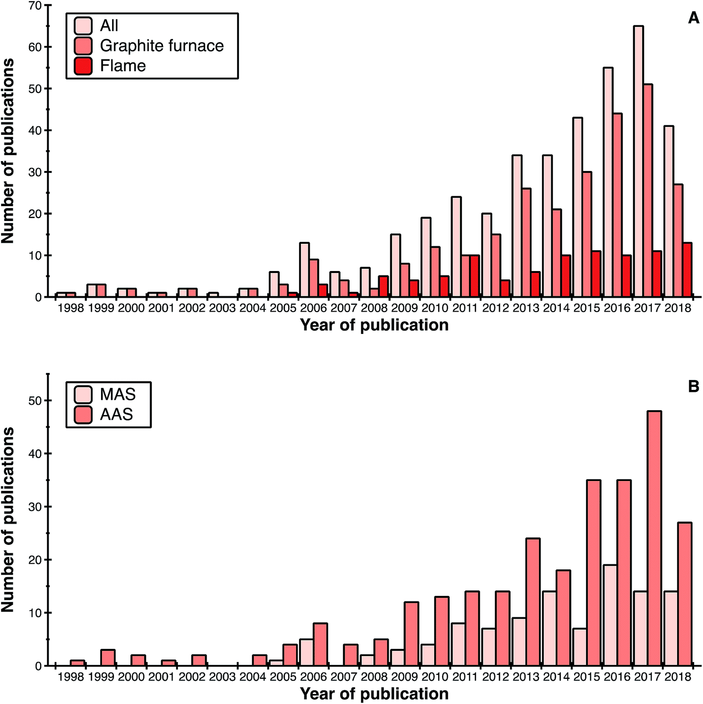

Fig. 1 Number of articles reporting on the use of HR CS depending on (A) the type of atomizer; and (B) the technique. Source: Scopus, September 2018. The search was carried out using the general term “high resolution continuum source” and the results were curated manually, in order to select only those related with the topic of the review.

If we focus on the type of atomizer, graphite furnace (GF) is the preferred one (selected in approximately 70% of publications), followed by flame (24%), as shown in Fig. 1a. Use of other atomizers (quartz, tungsten) is only residual. This could be anticipated, since graphite furnace and flame are the only commercially available atomizers, and graphite furnace offers superior potential in terms of sensitivity and capability to analyze samples directly when compared with flame. The latter is an important factor, as roughly 30% of the articles are devoted to direct analysis of solid or complex liquid samples. The number of articles using graphite furnace has continued to grow, while the number of those using flame seems to have reached a plateau over the last 4 years.

Regarding the measurement technique (see Fig. 1b), AAS articles are still predominant. Use of MAS, with its possibilities to determine non-metals, however, has been investigated in approximately 27% of the publications up to now. This type of research is still relatively new and the number of research groups exploring it is still limited.

Finally, an indication of the maturity of the technique is that, during the last decade, a significant number of papers have appeared in more applied journals, to the point that the articles published in these journals already represent 15–20% of the total number of HR CS AAS/MAS publications. While the term “applied” is always subjective, we are referring to journals devoted to food, clinical and environmental analysis. In particular, the number of articles appearing in journals devoted to food analysis is noteworthy. This number of applied publications will presumably continue to increase.

Overall, the field still shows potential to grow and has demonstrated possibilities to be applied to various fields.

3. Major research areas

This section will discuss the two current major areas of research, according to the number of articles published, which are the development of methods that enable direct analysis of samples (Section 3.1), and the development of methods for the determination of non-metals (Section 3.2). Those papers of higher novelty, in terms of methodology, will be highlighted. Tables 1 and 2 present the publications in both fields, respectively, starting from 2015. It also needs to be mentioned that those articles dealing with direct analysis while also targeting the determination of non-metals will be included only in Section 3.2 and in Table 2, in order to avoid duplications while achieving a better balance for both sections. For previous publications, the reader is referred to reviews on both topics published in 2014.^4,21

Table 1 Applications reporting on direct analysis using HR CS AAS since 2015. All of them used graphite furnace except for ref. 22

Analyte	λ (nm)	Chemical modifier	Type of sample	LOD/m0	Remarks	Ref.
Ag	328.07	No modifier	Biological matrices	—/—	Detection of Ag NPs based on atomization delay with respect to ionic silver. Study of the influence of the matrix with model matrices	71
Al	309.271	No modifier for Al; Pd(II) + Mg(II) nitrates for Si	Silicon carbide nanocrystals	0.5 μg L^−1/6.4 pg	External calibration with aqueous standards	27
Si	251.611			3 μg L^−1/389 pg
Al (AlH)	425.315	H2SO4 10% (v/v)	Soil samples	0.42 μg mg^−1/0.18 μg	All elements determined in the same sample aliquot. Cd was determined first at Tatom = 1700 °C. After changing the wavelength, Cr, Fe and Al (as AlH) were simultaneously determined at 2600 °C	29
Cd	228.802			7.3 pg mg^−1/3.9 pg
Cr	425.433			0.13 ng mg^−1/27 pg
Fe	425.076			0.07 μg mg^−1/0.09 μg
As	193.696	Pd(II) + Mg(II) nitrates + Triton X-100	Fish and seafood	0.05 μg kg^−1/20 pg	Maximum sample mass of 0.25 mg for avoiding matrix effects. Screening method for determination of inorganic As only. External calibration with aqueous standards	84
As	193.696	Zr (permanent modifier)	Soils	73 pg/22 pg	External calibration with aqueous standards	85
As	193.696	Ir (permanent modifier)	Marine sediments	0.02 ng/—	Calibration with solid reference materials. Fast temperature program with a short pyrolysis step	86
Cd	228.802			0.01 ng/—
Co	240.725			0.021 ng/—
Cr	359.349			0.015 ng/—
Cu	327.396			0.016 ng/—
Ni	341.477			0.011 ng/—
As	193.696	Ir (permanent modifier)	Marine biota samples	0.03 ng/40 pg	Fast temperature programs with short pyrolysis and drying steps. Calibration with solid reference materials. Least squares algorithm for correcting PO interference in As determination	87
Cd	228.802			0.014 ng/10 pg
Co	240.725			0.017 ng/77 pg
Cr	357.868			0.07 ng/66 pg
Cu	327.396			0.004 ng/77 pg
Ni	232.003			0.03 ng/12 pg
Au	242.795	No modifier	Geological samples	2.24 × 10^−6 μg g^−1/6 pg	Determination of Au after preconcentration of digested samples in carbon nanotubes. External calibration with aqueous standards	32
Cd	228.8	Pd(II) + Mg(II) nitrates	Facial make-up	0.0020 μg kg^−1/0.56 pg	External calibration with aqueous standards	88
Cd	228.802	Pd(II) nitrate	Lipsticks	5.0 pg/2.8 pg	External calibration with aqueous standards	89
Cd	228.801	No modifier	Ethanol fuels	0.006 mg kg^−1/C0 = 0.01 mg L^−1	Use of a flame atomizer. Multi-element fast sequential determination. External calibration with aqueous standards	22
Co	240.725			0.02 mg kg^−1/C0 = 0.06 mg L^−1
Cu	324.754			0.001 mg kg^−1/C0 = 0.02 mg L^−1
Fe	248.327			0.02 mg kg^−1/C0 = 0.05 mg L^−1
Mn	279.481			0.003 mg kg^−1/C0 = 0.01 mg L^−1
Na	589.592			0.1 mg kg^−1/C0 = 0.03 mg L^−1
Ni	232.003			0.04 mg kg^−1/C0 = 0.08 mg L^−1
Pb	217.000			0.06 mg kg^−1/C0 = 0.10 mg L^−1
Zn	213.857			0.024 mg kg^−1/C0 = 0.01 mg L^−1
Cd	228.802	No modifier	Tannin samples	0.5 μg kg^−1/0.3 pg	Sequential determination of Cd and Cr in the same sample aliquot. External calibration with aqueous standards	90
Cr	357.869			17 μg kg^−1/2.2 pg
Cd	228.802	No modifier	Yerba mate	0.25 ng/0.37 pg	Sequential determination for the same sample aliquot. External calibration with aqueous standards	91
Cr	357.869			0.72 ng/2.4 pg
Cd	228.802	Pd(II) + Mg(II) nitrates for Cd	Vegetables of the Solanaceae family	0.78 ng g^−1/0.42 pg	External calibration with aqueous standards	92
Cr	357.869			2.5 ng g^−1/2.7 pg
Cu	327.396			0.15 μg g^−1/19 pg
Cd	228.802	Pd(II) + Mg(II) nitrate for Cd; no modifier for Ni or V	Spices	0.2 ng g^−1/0.6 pg	Air-assisted pyrolysis step needed for enabling external calibration with aqueous standards	93
Ni	232.003			18 ng g^−1/14.0 pg
V	318.540			7 ng g^−1/18.6 pg
Co	240.725	No modifier	Wet animal feeds	0.051 μg g^−1/2.9 pg	External calibration with aqueous standards	94
Cr	357.869			0.009 μg g^−1/2.2 pg
Co	252.136	No modifier	High purity silicon	0.39 mg kg^−1/0.02 pg	External calibration with aqueous standards. Simultaneous determination of Fe and Ni	26
Fe	305.909			1.14 mg kg^−1/0.09 pg
Ni	305.760			5.71 mg kg^−1/0.54 pg
Co	304.400	Mg(II) nitrate for Ni. NH4F for Co and V	Soil	0.045 ng/0.093 ng	Co and V determined simultaneously. Different lines for Ni and Mo used for adjusting sensitivity. External calibration with aqueous standards feasible for all elements except Co. For Co, calibration with a solid reference material was carried out	95
Mo	313.259			5.4 pg/0.009 ng
Ni	341.347			1.8 ng/2.45 ng
	341.477			0.021 ng/0.045 ng
V	304.355			0.43 ng/0.43 ng
	304.494			0.59 ng/0.64 ng
Cr	357.869	Mixture of H2O2 + ethanol + HNO3 plus Mg(II) nitrate	Infant formulas	3.45 ng g^−1/1.2 pg	Mixture of modifiers needed for reduction of carbonaceous residues. External calibration with aqueous standards feasible	96
Cr	357.868	No modifier	Pharmaceutical drugs	2.9 μg kg^−1/2.0 pg	External calibration with aqueous standards	97
Cr	360.532	Ru (permanent modifier) + Pd(II) + Mg(II) nitrates + Triton X-100 for Pb	Industrial waste of oil shale and various reference materials	102 μg g^−1/25 pg	External calibration with aqueous standards	98
Cu	327.396			39 μg g^−1/19 pg
Pb	283.306			28 μg g^−1/24 pg
Cr	359.349	No modifier for Cr;	Sunscreen samples	1.0 μg kg^−1/2.5 pg	External calibration with aqueous standards	99
Pb	283.306	Pd(II) + Mg(II) nitrates in Triton X-100 for Pb		3.0 μg kg^−1/10 pg
Cr	427.5	Mg(II) nitrate in Triton X-100 (Cr);	Fertilizer samples	60 ng g^−1/88 pg	HR-CS GF AAS used to confirm the absence of spectral interference. Comparison with LS-GFAAS with the Zeeman effect	100
Tl	276.8	No modifier (Tl)		3 ng g^−1/11 pg
Cu	249.215	No modifier	Micro-volumes of distilled alcoholic beverages	0.03 mg L^−1/—	Calibration with matrix-matched liquid standards. Internal standardization with Cr, Fe and/or Rh feasible	101
Cu	327.396	KMnO4 for Hg; no modifier for Cu	Phosphate fertilizers	19 μg g^−1/25 ng	External calibration with aqueous standards	25
Cu	249.215			0.012 μg g^−1/1.12 ng
Hg	253.652			0.015 μg g^−1/39 ng
Cu	217.894	No modifier	Flours	0.11 mg kg^−1/14 pg	Simultaneous determination of the two analytes. External calibration with aqueous standards	102
Fe	217.812			0.03 mg kg^−1/77 pg
Cu	324.754	No modifier	Infant formula	0.003 μg g^−1/8.0 pg	External calibration with aqueous standards	103
Mn	403.076			0.01 μg g^−1/8.0 pg
Fe	352.614	Pd(II) nitrate	Solid magnetic nanoparticles	—/—	External calibration with aqueous standards. Method used for characterization of magnetic NPs	104
Fe	232.036	H2 gas admixed during pyrolysis	Fluoropolymers	221 ng g^−1/370 pg	Simultaneous determination of Fe and Ni. External calibration with aqueous standards	105
Ni	232.001			9.6 ng g^−1/7.7 pg
Fe	232.036	No modifier	Vegetables of the Solanaceae family	2 μg g^−1/340 pg	Simultaneous determination of Fe and Ni. Least squares algorithm for correcting interference from SiO. External calibration with aqueous standards	106
Ni	232.003			0.02 μg g^−1/95 pg
Fe	294.132	Ir (permanent modifier)	Fuel fly ash	3.19 ng/—	Simultaneous determination of Fe, Ni and V. External calibration with aqueous standards	107
Ni	294.391			1.20 ng/—
V	294.236			24.13 ng/—
Hg	253.652	Ir (permanent modifier)	Marine sediments and biota	0.025 ng sediments/—, 0.096 ng biota/—	Calibration with solid reference materials. Fast temperature program with a short pyrolysis step	108
Hg	253.652	Au NPs	Airborne particles	0.19 μg L^−1/0.004 μg L^−1	No pyrolysis step. Comparison of the effects of Ag and Au NPs as modifiers	109
Hg	253.652	Au nanoparticles	Blood and urine	2.3 μg L^−1/16 pg	External calibration with aqueous standards. Fast temperature program without pyrolysis	35
Li	610.353	No modifier	Yttrium oxyorthosilicate microsamples	20 μg g^−1/	Standard addition method for calibration	110
Na	285.301			80 μg g^−1/
Mg	215.435	No modifier	Lithium niobate crystals	0.7 mg g^−1/—	Calibration with powdered lithium niobate crystal standards	111
Mn	403.076	No modifier	Meat samples	0.005 μg g^−1/—	External calibration with aqueous standards for Mn. Calibration with solid reference materials for Ni and Rb. Least squares algorithm for correcting PO and SiO molecular interference in determination of Ni	112
Ni	231.096			0.002 μg g^−1/—
Rb	420.018			0.1 μg g^−1/—
Mn	403.076	No modifier	Powdered stimulant plants	0.05 μg g^−1/0.012 ng	External calibration with aqueous standards for Mn, Rb and Sr. Calibration with solid standards for Ni	113
Ni	231.096			0.02 μg g^−1/0.015 ng
Rb	420.018			0.1 μg g^−1/0.28 ng
Sr	407.771			0.01 μg g^−1/1.5 pg
Mo	313.259	No modifier	Plant materials	0.018 ng/0.12 ng	Simultaneous determination of Mo and Ni. Co used as an internal standard for avoiding matrix effects in Ni determination. External calibration with aqueous standards	31
Ni	313.410			0.025 ng/0.017 ng
Mo	313.259	No modifier	Reference materials of various natures	25 pg/7 pg	Atomization in disposable starch-based platforms made in-house for reducing tailing of the analyte signals. External calibration with aqueous standards	36
V	318.398			130 pg/18 pg
Pb	205.328	Pd(II) + Mg(II) nitrates	Glass	201.6 pg/1.6 ng	External calibration with aqueous standards compared with calibration with a NIST 612 glass sample. Both approaches provide similar results	114
	283.060			11.2 pg/0.1 ng
Pb	283.306	Pd(II) + Mg(II) nitrates	Eye shadow and blush	6 pg g^−1/—	External calibration with aqueous standards. Sample mass of 0.3 mg	115
Pb	217.001	Pd(II) + Mg(II) nitrates	Plastic food packaging	4.9 μg kg^−1/5.0 pg	External calibration with aqueous standards. Secondary line at 205.328 nm used for adjusting sensitivity	116
	205.328			0.5 mg kg^−1/0.4 ng
Pb	217.005	Pd(II) + Mg(II) nitrates	Plastic toys	0.037 mg kg^−1/9 pg	Ar gas flow during the atomization stage for adjusting sensitivity to the sample content. External calibration with aqueous standards	117
Pb	217.001	Pt chloride	Dried blood Spots	1 μg L^−1/26.6 pg	Screening method developed for Pb in DBS from newborns and pregnant women. External calibration with aqueous standards	118
Pb	217.001	No modifier	Biomass and products of the pyrolysis process	5 pg/4 pg	The line at 217.001 nm could not be used for some samples due to spectral interference. External calibration with aqueous standards	119
	283.306			9 pg/7 pg
Pb	283.306	Pd(II) + Mg(II) nitrates	Incense	Rod: 5.6 pg/8.2 pg, coating: 12 pg/29 pg	Analysis of rod and coatings of incense sticks. External calibration with aqueous standards for rods, but with solid matrix-matched standards for coatings	120
Pb	261.418	Pd(II) + Mg(II) nitrates + Triton X-100	Road dust and soil	0.65 mg kg^−1/1.20 ng	Investigation of molecules giving rise to spectral overlaps. Use of side pixels. External calibration with aqueous standards	121
	283.306			0.09 mg kg^−1/0.38 ng (using side pixels +4, −4)
Pd	360.955	No modifier for pharmaceuticals; NH4F·HF for catalysts	Automobile catalysts and active pharmaceutical ingredients	Pd, catalysts 6.5 μg g^−1/0.44 ng, pharm. 0.08 μg g^−1/0.18 ng	External calibration with aqueous standards for pharmaceuticals. Calibration with a solid reference material for the catalysts. Simultaneous determination of Pt + Rh and Pd + Rh feasible in both samples. An Ar flow of 0.1 L min^−1 during atomization used for analysis of catalysts	24
Pt	244.006			Pt, catalysts 8.3 μg g^−1/0.81 ng, pharm. 0.15 μg g^−1/0.32 ng
Rh	361.247			Rh (244.034 nm), catalysts 9.3 μg g^−1/0.84 ng, pharm. 0.10 μg g^−1/0.30 ng
Rh	244.034			Rh (361.247 nm), catalysts —/1.58 ng, pharm. 0.26 μg g^−1/0.68 ng
Rh	343.489	NH4F·HF	Spiked river water, road runoff and municipal sewage	1.0 μg L^−1/12.9 pg	Simultaneous determination of Rh and Ru. External calibration with aqueous standards	122
Ru	343.674			1.9 μg L^−1/71.7 pg
Sb	217.581	Pd(II) + Mg(II) nitrates	Cosmetics	0.27 mg kg^−1/0.028 ng	Study of different precursors for generating reference spectra for correcting the structural molecular background. Zeolite and mica were the most successful ones	123
Sb	217.582	Pd(II) nitrate	Waters subjected to micro-solid phase extraction with magnetic core-modified silver NPs	0.02 μg L^−1/—	Total Sb determination and determination of Sb(III) achieved by two extractions carried out at different acidities. Sb(V) calculated by difference. Comparison with the slurry approach. External calibration with aqueous standards	33
Si	221.174	Rh (permanent modifier) plus Pd(II) + Mg(II) nitrates in Triton X-100	Plant materials	2.5 ng/2.0 ng	Secondary line, Ar flow during atomization stage and absorbance in the center peak only used for adjusting sensitivity. External calibration with aqueous standards	124
Si	251.611	Rh (permanent modifier) plus Pd(II) + Mg(II) nitrates	Biomass and products of the pyrolysis process	0.09 mg kg^−1/0.3 ng	External calibration with aqueous standards	125
	221.174			3 mg kg^−1/2 ng
Tl	276.786	Pd(II) nitrate	Spruce needles	1.2 μg kg^−1/—	Comparison of four methods of analysis	126

---

Table 2 Applications reporting on the determination of non-metals using HR CS MAS since 2015

Vaporizer	Analyte	Species monitored	λ (nm)	LOD/m0	Chemical modifier	Type of sample	Remark	Ref.
Graphite furnace	Br	Ca^79Br	600.492	4.0 ng/—	Pd nanoparticles	CRMs: PVC and tomato leaves	Isotopic analysis of Br. Direct solid sampling with ID calibration	55
		Ca^81Br	600.467
		CaBr	625.315
Graphite furnace	Br	CaBr	625.315	10 μg g^−1 (LOQ)	Zr (permanent modifier) + Pd	6 polymeric CRMs	Direct solid sampling. Comparison with LA-ICP-MS	127
Graphite furnace	Br	TlBr	342.982	0.3 ng/4.4 ng	Ag	Water	Direct analysis. The modifier prevents losses of Br through precipitation as AgBr	56
Graphite furnace	Cl	Al^35Cl	262.238	0.25 mg L^−1/—	Pd	Water CRMs and mineral waters	Isotopic analysis of Cl. ID for calibration	54
		Al^37Cl	262.222
Graphite furnace	Cl	SrCl	635.862	0.85 ng/0.24 ng	Zr (permanent modifier)	Coal (5 CRMs)	Direct solid sampling. External calibration with aqueous standards	128
Graphite furnace	Cl	AlCl	261.418	2.1 ng/0.28 ng	Zr (permanent modifier)	NIST 1634c fuel oil, crude oils	Direct analysis. External calibration with aqueous standards. Sr also added to increase the sensitivity for AlCl and InCl molecules	129
		InCl	267.281	3.5 ng/1.7 ng
		SrCl	635.862	0.7 ng/1.0 ng
Graphite furnace	Cl	InCl	267.217	0.10 ng /0.21 ng	Pd + Mg	Water samples, a diclofenac pill and CRM QC 1060 anions-WP	Non-spectral interference in the presence of other halogens	130
Graphite furnace	Cl	SrCl	635.862	1.76 μg mL^−1/—	Zr (permanent modifier)	Milk and one CRM (wastewater)	Dilution of the sample to adjust the sensitivity. External calibration with aqueous standards	131
Graphite furnace	Cl	CaCl	620.862	0.75 ng/0.072 ng	Pd	CRMs of varying nature	Direct solid sampling. External calibration with aqueous standards	50
			377.501	14.2 ng/25.9 ng
Graphite furnace	Cl	CaCl	621.145	1.4 ng/—	No modifier	Cement	Direct solid sampling. External calibration with aqueous standards. Ca compounds present in cement samples acted as the CaCl-forming reagent	132
Graphite furnace	Cl	SrCl	635.862	1.8 ng/0.32 ng	Zr (permanent modifier)	Fish oil samples	Dilution with L-propanol. External calibration with aqueous standards	133
Graphite furnace	Cl	MgCl	377.010	1.7 ng/7.1 ng	W (permanent modifier) + Pd	Water samples from an offshore oil platform and two CRMs	Wall vaporization. Direct analysis of water samples. External calibration with aqueous standards	52
Graphite furnace	Cl	MgCl	377.010	3.0 μg g^−1/—	W (permanent modifier) + Pd	Crude oil samples and NIST 1634c (fuel oil) and NIST 1848 (lubricating oil)	Analysis after emulsification. External calibration with aqueous standards	134
Graphite furnace	Cl	GaCl	249.060	2.3 ng/6.5 ng	Zr (permanent modifier), Pd(II) + Mg(II) in solution	Milk, mineral water and a certified wastewater sample	GaCl vaporizes at a low temperature (1100 °C)	51
Graphite furnace	F	CaF	606.440	0.3 ng/0.1 ng	Pd (permanent modifier)	Coal CRMs	Direct solid sampling. Comparison of different modifiers. External calibration with aqueous standards	135
Graphite furnace	F	CaF	606.440 + 606.231	0.18 ng/0.058 ng	No modifier	Turkish wines	Summation of the absorbances at two λ in order to increase the sensitivity and reduce the LOD	136
Flame	F	AlF	227.66	—/—			Research on how the chemical form of F species affects the sensitivity of AlF	59
C2H2/N2O		BF	195.59	—/—
Graphite furnace	F	CaF	606.045	2 mg kg^−1/0.68 ng	No modifier	Eye shadow samples and two CRMs	Direct solid sampling. External calibration with aqueous standards	137
Graphite furnace	F	CaF	606.440	0.20 ng/0.17 ng	No modifier	Baby food and one CRM (bush branches)	Direct solid sampling. External calibration with aqueous standards	138
Graphite furnace	F	CaF					Thermodynamic simulation of the mechanism of formation of CaF	139
Graphite furnace	F	CaF	606.440	0.22 ng/0.16 ng	No modifier	Flour samples and one CRM (bush branch NCS DC 73349)	Slurry sampling. External calibration with aqueous standards feasible	140
Graphite furnace	F	CaF	606.432	—/—	Pd (permanent modifier)	Airborne particulate matter (PM10) and CRMs (NIST 1648 and 1648a)	Direct solid sampling. Determination of Cl, Br and I by ETV-ICP-MS	141
Graphite furnace	F	SrF	651.187	0.36 ng/—		PM2.5 airborne particulates and wastewater CRM	Determination of F in particulate loaded quartz filters	142
Graphite furnace	F	CaF	606.440	0.72 ng mg^−1/0.13 ng	No modifier	Soil samples and one CRM (lake sediment)	Direct solid sampling. External calibration with aqueous standards	143
Graphite furnace	F	CaF	606.440	0.13 ng mL^−1/—	No modifier	Herbs, water samples and various CRMs	Use of slurries combined with preconcentration on nano-TiO2 prior to injection to HR CS MAS. External calibration with aqueous standards	144
Graphite furnace	F	GaF	211.248	8.1 μg L^−1/—	Pd/Mg + Zr + CH3COONa	Surface waters and two river water CRMs	Comparison with ion chromatography. HR-CS-GFMAS offers higher throughput, a lower LOD and higher selectivity	145
Graphite furnace	F	SrF	651.187	30 μg L^−1/—		Mineral waters and a water CRM	Chemical interference was caused only by high chlorine concentrations	146
Graphite furnace	F	CaF	606.440	—/—	No modifier	Tea leaves	Study of the mechanism of formation of CaF	58
Graphite furnace	F	CaF	583.069	0.1 ng/—	Zr (permanent modifier)	Sweat samples of cancer patients	Use of mini graphite tubes with low sample consumption (down to 30 nL)	82
			606.440	0.01 ng/0.1 ng
Graphite furnace	I	CaI	638.904	0.041 mg g^−1/23 ng	Pd/Mg	Pharmaceutical (one liquid drug and sodium levothyroxine pills)	Even a low Cl concentration reduces the absorbance of both molecules significantly. External calibration with aqueous standards and standard addition (pills)	57
		SrI	677.692	0.021 mg g^−1/18 ng
Graphite furnace	NO2^− + NO3^−	NO	215.360	0.16 mg dm^−3/—	Ca	Water CRM	Total NO2^− + NO3^− content monitoring NO	147
Graphite furnace	NO2^− + NO3^−	NO	215.371	0.3 mg L^−1/—	Ca	Herbal infusions	Standard addition method for calibration	148
Quartz cell	NO2^− + NO3^− + PNP	NO	215.360	0.16 mg dm^−3/—	Ca	Food and water samples	Speciation method for nitrite, nitrate and p-nitrophenol via photochemical vapor generation. Nitrate and p-nitrophenol need to be reduced to nitrite first to be determined	60
Graphite furnace	P	P2	204.205	7 ng/10 ng	Zr (permanent modifier) plus sodium tetra-borate	CRMs (Spinach leaves and pine needles) and serum reference materials	Use of P2 enables gentle temperature conditions and multi-line evaluation to improve the LOD	80
Flame C2H2/air	P	PO	327.04	1.0 mg L^−1/—	Al	Ferrovanadium sample and CRM	Ca and Mg interfere, but Al reacts with them forming stable compounds and eliminating the interference	149
Graphite furnace	P	PO	213.561	2.35 mg g^−1/—	Mg	Soybean lecithin samples	Samples diluted in MIBK. The signal was obtained by summing four PO lines surrounding 213 nm to increase the sensitivity	150
			213.526
			213.617
			213.637
Flame C2H2/air	S	CS	258.056	1.5 mg g^−1/—		Food samples and CRMs	Microwave-assisted digestion of samples	151
Graphite furnace	S	CS	258.056	7.5 ng/8.7 ng	Ru (permanent modifier) plus Pd and citric acid	Vegetables and CRMs	Direct solid sampling. External calibration with aqueous standards prepared with thioacetamide	152
Graphite furnace	S	CS	258.056	1.4 mg kg^−1/17 ± 3 ng	Ir (permanent modifier) plus Pd/Mg	Diesel fuel samples and CRMs	Dilution of samples with L-propanol. External calibration with aqueous standards prepared with L-cysteine	153
Flame C2H2/air	S	CS	257.961	52.4 mg kg^−1/—		Preserved fruits	A method to detect SO2 in this kind of sample	154
Flame C2H2/air	S	CS	258.056	25 mg L^−1/—		Bovine serum albumin and L-cysteine	During MW digestion S is converted to SO4^2− prior to the determination. Standard addition method for calibration	155
Flame C2H2/air	S	CS	258.056	11.6 mg L^−1/—		Vinegars	Due to non-spectral interference, all sulfur species were oxidized to SO4^2−. Standard addition method for calibration	156
Graphite furnace	S	CS	258.056	0.0001% (w/v)/—		Particulate loaded filter samples and one CRM	PM2.5 airborne particulates collected in quartz filters	157
Graphite furnace	S	SnS	271.624	5.8 ng/13.3 ng	Pd	Crude oil samples and CRMs	Samples were prepared as a micro-emulsion due to their high viscosity. External calibration with aqueous standards	158
Graphite furnace	S	CS	258.056	0.018%/—	No modifier	Human hair samples and two hair CRMs	Correlation of sulfur levels of autistic children's hair with total protein and albumin	159
Graphite furnace	S	SiS	282.910	—/15.7 ng	Zr (permanent modifier) plus sodium tetra-borate		GeS provides the best sensitivity while PbS offers the lowest sensitivity and a low bond strength	44
		GeS	295.209	—/9.4 ng
		SnS	271.578	—/20 ng
		PbS	335.085	—/220 ng
Graphite furnace	S	CS	258.033	0.30 mg g^−1/—	W (permanent modifier) plus KOH	Petroleum green coke samples and a CRM (NIST 2718)	Slurry sampling. External calibration with aqueous standards prepared with thiourea	160
Quartz cell	Free and total S(IV)	SO2	215.356	0.36 mg L^−1/—		Coconut water	Measurement of SO2 generated after the addition of HCl. For total S, NaOH was added before to release the sulfite bound to organics. Summation of three SO2 transitions to improve sensitivity	61
			215.416
			215.486
Graphite furnace	S	CS	258.056	6 ng/—	Zr (permanent modifier) plus Ca and Pd	Milk, orange juice, swamp water, urine and two biological CRMs	Direct analysis of liquid samples and digestion of the solid CRMs. External calibration with aqueous standards	161
Graphite furnace	S (as proxy for cysteine)	CS	258.034	0.4 mg kg^−1/—	Pd/Mg	Pharmaceutical formulations and a CRM (NIST 1573a)	Summation of two CS transitions	162
			258.056
Graphite furnace	S	CS	257.958	23 ng/—	Pd/Mg	Apricot and grape samples and a CRM (NIST 1568a)	258.056 nm line not used due to potential overlap with the Fe line	163

---

3.1. Direct analysis of samples

This remains the most popular research area. As mentioned in the previous section, approximately 30% of all the papers devoted to HR CS AAS/MAS focused on this topic. The percentage would be higher (roughly 40%) if only graphite furnace articles are taken into account, since, obviously, flame is not as suitable for direct analysis (although it also shows some potential: one study by Leite et al.²² demonstrated that it is possible to carry out the direct analysis of ethanol fuel, determining 9 analytes).

It has to be stated that by direct analysis we are not referring to solid sampling only, but also to those other papers in which generally complex liquid samples can be analyzed directly. In fact, in such cases, the procedure used is sometimes very similar to that of solid sampling (e.g., deposition of the sample onto the external platform). However, in practice, almost 90% of the articles are actually devoted to the analysis of solid materials.

It certainly makes sense that solid sampling HR CS GFAAS/MAS is a major area of research because this technique is particularly suitable for such an approach. This was, in fact, the topic of one previous review published in JAAS in 2014.²¹ The temperature control, the potential for chemical modification, and the possibilities of the technique to detect and deal with spectral overlaps make it possible in many occasions to analyze difficult materials and even to simply use aqueous standards to construct the calibration curve (an approach that will be referred to as external calibration with aqueous standards from now on). This characteristic is quite unique in comparison with many of the other solid techniques that require solid standards for calibration.²³ One may in fact wonder if this technique could become the method of choice for trace element analysis of solid samples, letting aside imaging applications, if higher multi-element capabilities would be available at some point, but this topic will be discussed in Section 4.3.

An examination of the recent literature on direct analysis using HR CS GFAAS/MAS (see Table 1) reveals a period of maturity. From a methodological point of view, practically all that was discussed in the review mentioned before²¹ holds true. The technique has shown potential to analyze very different types of materials, from some that could be considered as relatively easy for graphite furnace decomposition, such as polymers, biological materials or pharmaceuticals, to others that are quite refractory and, also, very difficult to bring into solution quantitatively, such as automobile catalysts,²⁴ fertilizers,²⁵ high-purity silicon²⁶ or silicon carbide,²⁷ in addition to many types of environmental samples.

A significant number of the articles presented in Table 1 (twelve studies) have reported the simultaneous determination of two analytes, or else their sequential determination, but from the same sample aliquot. Thus, this is an aspect that continues being investigated, even though the main characteristics that the analytes need to exhibit and the key aspects for optimizing the analytical procedure for such type of determination have already been well-established before.²⁸

The most interesting and elegant of these approaches, in the authors' opinion, was published by Boschetti et al.,²⁹ as it takes advantage of various possibilities to achieve the determination of four different elements in soil samples. In that paper, the determination of Al, Cr, Cd, and Fe was aimed at. These elements do not show atomic lines sufficiently close to be simultaneously monitored by HR CS AAS instrumentation (see Section 4.3 for further discussion on this topic). However, as already discussed by Resano et al.,¹⁸ it is often not as important to determine the analytes in a truly simultaneous fashion, as it may be to determine them from the very same sample aliquot. Since Cd is much more volatile than the other analytes, it is possible to atomize first this element at 1700 °C and monitor it using the main Cd line (228.802 nm), and then change the wavelength, increase the temperature and vaporize/atomize the rest. There is an alternative line for Cr (425.433 nm) that is suitable for the expected analyte content, and very close to it there is an Fe line (425.076 nm), also appropriate for the expected sample concentrations. That is not so surprising giving the abundance of Fe lines over the whole UV-vis spectrum. There is no Al line close, but there are rotational lines corresponding to AlH that are found in the vicinity. It has to be remembered that molecular lines can be used not only to determine non-metals, but in some occasions, it may be beneficial to use them for metals as well, as shown in the past using AlF to determine Al.³⁰

Summing up, by using both a sequential (Cd atomization first) and later a simultaneous (Cr and Fe atomization) AAS approach, combined with MAS (AlH simultaneous monitoring), the authors managed to determine four elements in every single aliquot of soil samples directly, using external calibration with aqueous standards, which is remarkable. It is certainly not common to be able to deploy simultaneously two different techniques with the same instrument, but that is an existing possibility that should be explored in more HR CS AAS/MAS applications.

The use of an internal standard (IS) is related to this topic of simultaneous monitoring. A work by De Babos et al.³¹ demonstrated how the use of cobalt as an internal standard helps in circumventing matrix effects for the simultaneous determination of Ni and Mo in plants. In fact, the use of this IS was only necessary for Ni, as the sensitivity obtained for aqueous solutions and for solid samples was found to be significantly different. Co was selected as an IS since it shows an atomic line (313.221 nm) close to those used for Ni (313.410 nm) and Mo (313.259 nm) and, also, because its thermochemical properties are very similar to those of Ni. The suitability of Co as an IS for Ni determination by HR CS GFAAS has already been demonstrated in the literature.¹⁸ This is probably the first time, however, that such an approach is used to perform direct solid sampling via HR CS GFAAS. The IS was added in solution, and its use enabled accurate results to be obtained for all the plants investigated using external calibration with aqueous standards.

Another topic that could be mentioned is the possibility to use solid sampling HR CS GFAAS after some sample preparation. Obviously, in that way, some of the intrinsic advantages of direct analysis are lost, but some benefits can also be obtained. For instance, it is possible to preconcentrate the analyte in a solid phase and analyze such solid phase without any dilution. One example of this approach was published by Dobrowolski et al.,³² who reported the use of modified carbon nanotubes for the solid-phase extraction of Au in a digest of geological samples, with the subsequent SS HR CS GFAAS analysis, resulting in an enrichment factor of 100.

A similar idea but adding speciation potential to the preconcentration efficiency was described by López-García et al.³³ They proposed a micro-solid phase extraction procedure, based on magnetic nanoparticles covered with Ag nanoparticles and functionalized. This magnetic character enables an easy separation of the solid phase containing the analytes, which can then be directly analyzed via SS HR CS GFAAS, or else slurried and injected into the furnace, achieving enrichment factors of 325 and 205, respectively. Moreover, by controlling the pH during the extraction, quantitative information on both total Sb (pH = 2) and Sb(III) only (at pH = 9) can be achieved, such that the amount of Sb(V) can be calculated by difference. A similar speciation approach, but not using solid sampling this time, was reported by the same research group to determine both total Cr and Cr(III) only (and thus, Cr(VI) by difference), which were retained in a graphene oxide suspension.³⁴

Use of nanomaterials/nanoparticles is, therefore, also enabling some improvements in HR CS AAS procedures. Another recent example was reported by Aramendía et al.,³⁵ who proposed the use of AuNPs aiming at the direct determination of Hg in blood and urine via HR CS GFAAS. The rationale is that one of the challenges for Hg determination is the extreme volatility of Hg(0), for which use of an oxidizing agent (e.g., KMnO₄) as a chemical modifier is common. However, it is well-known that Hg(0) amalgamates with Au. Thus, instead of preventing Hg(0) formation, it may be beneficial to favor it, and already have Hg in the metallic state, thermally stabilized by means of this interaction with AuNPs to avoid any losses during the drying step, but ready for fast atomization at a low temperature (500–700 °C), before the bulk of the matrix is released. This approach basically eliminates the pyrolysis step, resulting in a very fast temperature program and yet improved sensitivity, because the samples are not diluted.

HR CS GFAAS can also be deployed for quantifying and even for sizing NPs, but this topic will be covered in detail in Section 4.2.

The last topic worth mentioning in relation with direct analysis is the use of a disposable platform made of corn starch and sorbitol, as proposed by Colares et al.³⁶ This platform permits the transport of the solid sample to the graphite tube, but then it decomposes during the pyrolysis step, so the final effect is similar to using wall atomization. This is beneficial for refractory elements, as it minimizes tailing, enabling atomization in shorter times, thus enhancing the lifetime of the tubes. The reduction of memory effects also improves precision. Mo and V were chosen to prove these concepts and were successfully determined in different reference materials.

3.2. HR CS MAS for determination of non-metals

An examination of the recent literature (since 2015) shows that the elements more often determined via HR CS MAS are F, S, and Cl, in that particular order. The articles devoted to these elements represent approximately 80% of the total number in this period. These results can be explained considering the importance of the elements, the possibilities to determine them via HR CS MAS, and the difficulties observed for competing techniques.

For instance, F and S were already the most investigated elements in previous years using HR CS MAS.⁴ This is not so surprising as F forms very stable bonds (typically the most stable ones among halogens), favoring the formation and persistence of diatomic molecules at the high temperatures used in the atomizers. Moreover, the sensitivity of these molecules is rather high and the determination of F by competing techniques is complicated (e.g., F does not get positively ionized in an inductively coupled plasma (ICP), making the use of ICP-mass spectrometry (MS) poorly suitable to determine this element at trace levels³⁷), while HR CS GFMAS can provide LODs of a few picograms only when the most sensitive molecule (GaF) is used.^38–41 Therefore, HR CS MAS is an important tool to quantify F traces.⁴² However, the literature shows that the popularity of this molecule has decreased very much in favor of CaF, which has been selected in more than 70% of the articles published since 2015. The main reasons for this are discussed by Morés et al. when they first reported on the use of CaF.⁴³ Targeting CaF does not require a complex mixture of modifiers, as in fact Ca acts as both a modifier and molecule forming reagent. Moreover, the CaF main absorption head is found in the visible (606.440 nm) region of the spectrum (GaF is measured at 211.248 nm), where spectral interference is rare. Thus, unless required by the analyte content (use of CaF results in roughly two orders of magnitude lower sensitivity), most studies preferred the simplicity of monitoring CaF.

In the case of S, the most favored molecule continues to be CS, except in a few specific cases. Possibilities of other molecules will be discussed in Section 4.3.⁴⁴ It is interesting to note that the majority of articles discussed in this section propose the use of the graphite furnace, but in the case of S determination, several articles demonstrate the benefits of using flame or quartz vaporization. This is mostly because S needs to be determined at trace levels, and a cheap and fast approach for S determination at higher levels is useful, particularly for food control.

Investigations on P have significantly decreased in comparison with previous years.⁴ This is however not so rare because many of the previous P papers corresponded to basic research in which the problem of the potential appearance of both atomic and molecular (PO) lines was analyzed in detail depending on the type of modifiers, conditions used and/or BG correction method. In fact, the appearance of HR CS GFAAS instrumentation served to explain many of the issues associated with P monitoring by AAS.^45,46 Since the situation is now clear and the conditions to determine this analyte, either as P or as PO and even using direct solid sampling, are well-established,⁴⁷ a lower production of articles can be seen as normal.

Cl, on the other hand, has been the subject of more research in the period covered. This fact is very welcome. Actually, one review on the determination of non-metals published in 2014 noted the surprisingly low number of papers devoted to Cl determination via HR CS MAS, despite the importance of this element.⁴ Three new molecules have been proposed in this period to accompany the ones previously explored (AlCl,³⁸ InCl,⁴⁸ and SrCl⁴⁹), namely CaCl,⁵⁰ GaCl⁵¹ and MgCl.⁵²

Having different molecules to choose from for every particular application is important. Nevertheless, the increasing popularity of Ca, already noted for F and also the main choice for Br determination, is noteworthy. CaX (where X represents a halogen) molecules typically offer various (but not too many) transitions of different sensitivities in the visible region, making it easy to set the baseline, adjust the working range and minimize spectral interference. Moreover, Ca is an element present at high content in many types of samples (e.g., biological), so it could cause strong interference if any other molecule is targeted instead.⁵⁰ Use of Ca also represents some disadvantages in practice, as this element is well known to deteriorate the lifetime of the graphite parts.⁴³

Determination of Br and, particularly, I is more challenging because their bonds with metals are much less strong than those of F and Cl. Thus, determining them in samples in which the presence of F and/or Cl is significant can be problematic.⁵³ A potential solution for such a situation based on the use of isotope dilution will be discussed later.^54,55 Recently, the use of TlBr has been proposed for Br determination,⁵⁶ as well as the use of CaI and SrI for I determination.⁵⁷ In any case, for these two elements, more research on the use of different molecules is needed.

Another topic that requires further research is the way in which the different modifiers and molecule forming agents interact with the analyte. It has to be considered that former studies on chemical modification were mainly carried out to investigate the best ways to achieve the atomization of metals. Therefore, there is not so much information on situations in which the analyte is a non-metal and the goal is to ultimately form a molecule in the gas phase. It is not so clear, for instance, when using a classical combination of modifiers (e.g., Pd and Mg), plus Ca as a molecule forming agent, which element will interact with the target non-metal and how, and if the targeted molecule will be formed first in the solid phase, or only later on in the gas phase.⁵⁸ Supplementary research in this area may enable the development of better general strategies to determine non-metals using HR CS MAS.

Finally, a significant number of articles (fifteen, representing almost 30% of the studies shown in Table 2) have demonstrated the potential of the technique for direct analysis of solid and complex samples (and that is not counting approaches based on slurries), also when targeting non-metals. Direct analysis may be particularly beneficial in this field because sample pretreatment is particularly problematic owing to the volatility of many species in which the non-metals are usually found, and the problems associated with contamination. In fact, the signal obtained for non-metals might be significantly affected by the way in which they are found in the sample,⁵⁹ and the way in which such samples are pretreated. This is a challenge when aiming at bulk analysis, but it can be transformed into an advantage to perform some speciation studies. Two recent articles have reported on the determination of nitrite, nitrate, and p-nitrophenol⁶⁰ and free and total sulfur(IV)⁶¹via the selective formation of volatile species after suitable sample treatment and the monitoring of NO and SO₂, respectively, using HR CS MAS with a quartz vaporizer in both cases.

4. New possibilities

Apart from these major areas, there are some new and intriguing possibilities that have appeared more recently and are covered in a few papers only. They are, however, worth commenting on because they may have a significant effect in the future use of the technique.

4.1. Isotopic analysis via molecular monitoring

It has been well-documented for years that it is, in principle, possible to use atomic absorption to obtain isotopic information because the atomic lines of different isotopes do not appear at exactly the same wavelength. However, in practice, being able to appreciate these transitions separately is very challenging. The differences among isotopic lines are very small (a few picometers only) and, furthermore, even if such a high resolution is attainable, it has to be considered that broadening of the peaks due to different effects (i.e., collisional broadening, and Doppler and Stark effects) occurs, further complicating the separate monitoring of isotopic lines.

It is therefore not surprising that only one paper to date has made use of HR CS AAS for isotopic analysis. In that study, Wiltsche et al. focused on boron isotopes.⁶² This selection is not casual. For such a light element, the mass difference between ¹⁰B and ¹¹B atoms is quite significant, and therefore, the isotopic shift should be much larger. In fact, Wiltsche et al. discussed that it was preferable to use the less sensitive atomic line observed in the vicinity of 208.9 nm because the isotopic shift of this transition was higher than that observed for the B main line, found at approximately 249.8 nm. This loss of sensitivity in order to achieve better spectral resolution is a compromise that will be necessary also when using MAS, as will be discussed below, somewhat limiting the applicability of the method. The goal of the work was the determination of boron isotopes in steel, which could be done for samples containing at least 1% of boron, or else, a preconcentration was required.

To provide an idea of the small differences that we are discussing when it comes to atomic isotopic shifts, the line for pure ¹⁰B has been reported to be found at 208.95898 nm and, for pure ¹¹B, at 208.95650 nm. In practice, it was not possible to observe two fully resolved peaks with the HR CS AAS instrument, as could be anticipated for the reasons discussed above (broadening effects). What could be appreciated was that the peak maximum of the boron absorption line shifted as a function of the boron isotopic ratio, moving towards higher wavelengths with higher ¹⁰B content.

It has to be mentioned that the authors used a flame as the atomizer. Use of a graphite furnace could improve sensitivity, but it has to be remembered that boron is a defying analyte for GFAAS⁶³ and, also, that the authors simultaneously monitored either Fe or Ni lines, together with those of boron, because the use of an internal spectral standard was recommended to correct for instabilities of the monochromator (such as wavelength drifts and changes in the optical resolution). This truly simultaneous monitoring is easier to perform with a flame because with a graphite furnace there would be a delay between the atomization of Fe or Ni and the atomization of a refractory element, such as boron.

In the end, the method proposed was deemed satisfactory as a cheap and simple approach for the identification of steel scrap enriched in ¹⁰B, accepting an uncertainty level of 5% for the ¹⁰B content.

However, it has been proposed more recently that, if instead of using HR CS AAS, HR CS MAS is chosen, the isotopic analysis potential could be enhanced.⁵⁴ This seems like a logical evolution for two reasons: (i) MAS is an important area of research in this particular field of high-resolution continuum source, as discussed before, because diatomic molecules can be formed and their spectra resolved; (ii) it has already been shown for laser induced breakdown spectrometry (LIBS) by Russo et al. that the monitoring of molecular spectra provides higher isotopic shifts.^64,65 Therefore, the same idea could also be applied to HR CS MAS.

And this idea was demonstrated for Cl using a graphite furnace as the vaporizer. Al was chosen as the counterion in solution, in order to form the AlCl molecule in the gas phase. The selection of Al was based on several aspects: (i) AlCl is a stable molecule (bond dissociation energy, 511 kJ mol⁻¹), even at high temperatures; (ii) it shows good sensitivity, as reported before;³⁸ (iii) Al is monoisotopic, which is always preferable, as the shifts will thus only depend on Cl isotopes; and (iv) the shift observed for Al³⁵Cl and Al³⁷Cl lines is significant.

This shift can be predicted with accuracy using the first three terms of the following equation, which was proposed by Herzberg:⁶⁶

In that equation, Δν is the isotopic shift expressed in cm⁻¹, v stands for the vibrational quantum number, ω_e represents the harmonic frequency, ω_ex_e is the first anharmonic constant and ω_ey_e is the second anharmonic constant. As for the term ρ it equals (μ/μⁱ)^1/2, where μ is the reduced mass of the molecule and i corresponds to the heavier isotope. The number of apostrophes denotes the electronic levels involved in the electronic transition: two for the lower one, and one for the upper one.

As shown in Table 3, the shift can be predicted with great accuracy, as demonstrated by the excellent agreement found between theoretical and experimental values.

Table 3 Theoretical and experimental isotopic shifts calculated and observed via HR CS GFMAS, respectively, for the analytical band heads of the AlCl molecule (X¹Σ⁺ → A¹Π electronic transition) for different vibrational transitions (v′, v′′). Reproduced with permission from the Royal Society of Chemistry (https://pubs.rsc.org/en/content/articlehtml/2015/ja/c5ja00055f)⁵⁴

λ/nm	λ exp/nm	v′, v′′	Δλcalc/pm	Δλexp/pm	Relative sensitivity/%
261.44	261.418	0, 0	1.37	—	100
261.70	261.695	1, 1	4.86	4.8	62
261.82	261.819	2, 2	9.61	9.6	30
262.24	262.238	3, 3	16.0	15.6	26
262.70	262.697	4, 4	24.2	24.3	16
263.22	263.216	5, 5	34.8	35.3	7.4
263.81	263.807	6, 6	48.0	48.1	3.2
264.49	264.490	7, 7	64.3	64.5	1.1

---

Unfortunately, the magnitude of the shift was found to be inversely proportional to the sensitivity of the transition, as it is related to the vibrational level. Higher vibrational levels produce higher shifts, but also lower sensitivities because their population is also lower.

This can be seen both in Table 3 and, more visually, in Fig. 2, which shows the signals obtained for different transitions. The 261.418 nm transition, the most sensitive one, is not useful for isotopic analysis, as the signals for the two isotopes are not resolved (see Fig. 2A). The next transition, 261.695 nm, still does not show two different peaks, but the exact wavelength of the maximum depends on the isotopic composition (see Fig. 2B), shifting to higher values with higher ³⁵Cl content. The next transition already shows two separate peaks (see Fig. 2C), but they are not perfectly resolved. The resolution further improves (in Fig. 2D the ratio of the peaks is already correct, close to 1) for the next transitions, although for the last one the sensitivity is too low for the Cl content used in the experiment.

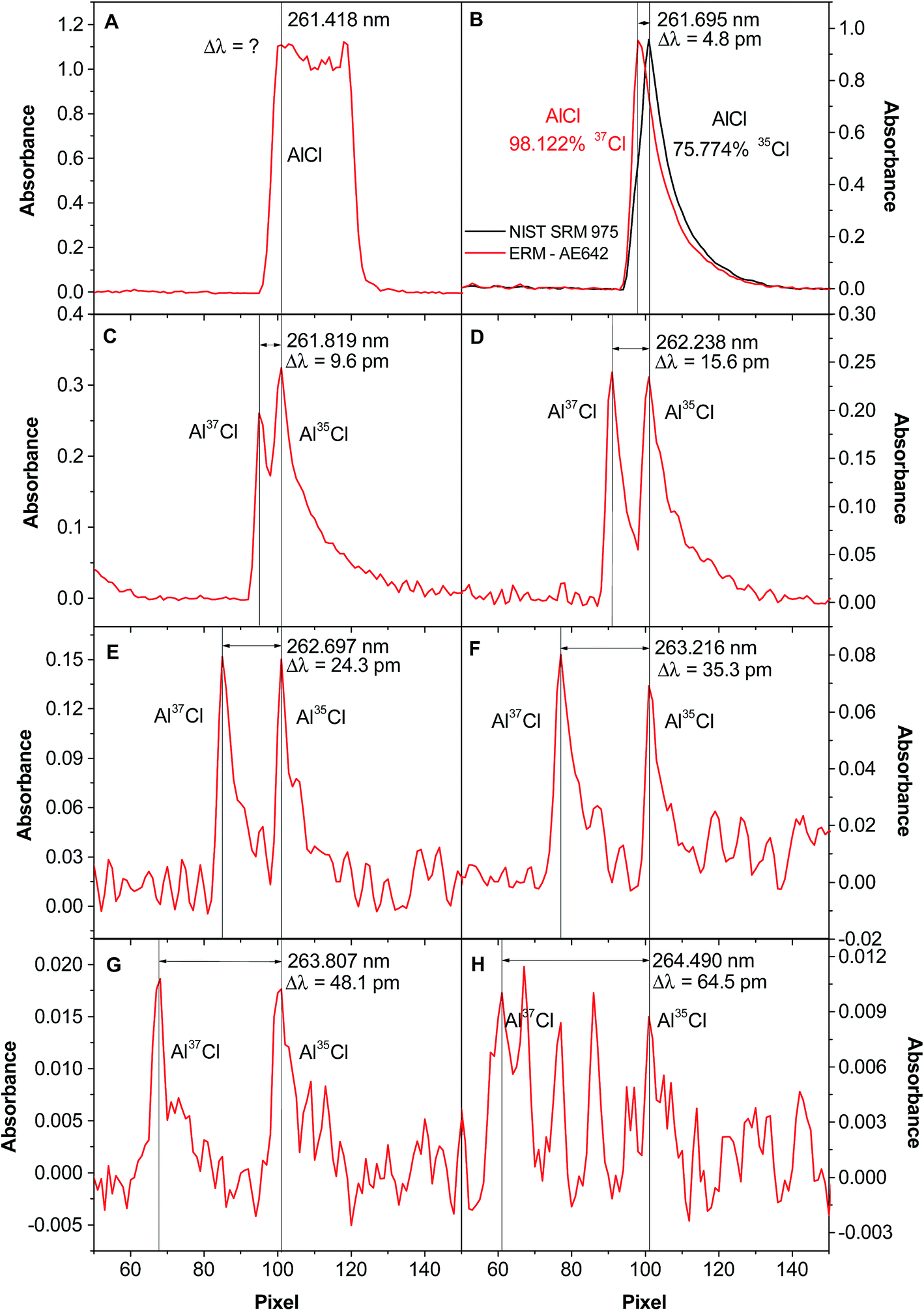Fig. 2 Spectra of AlCl when vaporizing 400 ng of Cl from an approximately 1 : 1 ³⁵Cl/³⁷Cl molar ratio solution, in the presence of 10 μg Al and 20 μg Pd, and monitoring the following wavelengths via HR CS GFMAS: (A) 261.418 nm; (B) 261.695 nm; (C) 261.819 nm; (D) 262.238 nm; (E) 262.697 nm; (F) 263.216 nm; (G) 263.807 nm; and (H) 264.490 nm. In Fig. 1B, the spectrum obtained for CRM NIST 975a (³⁵Cl 75.774%) is shown in black, and the one obtained for CRM AE642 (³⁷Cl 98.122%) is highlighted in red. Reproduced with permission from the Royal Society of Chemistry (https://pubs.rsc.org/en/content/articlehtml/2015/ja/c5ja00055f).⁵⁴

Fig. 3A shows that the transition selected and the way in which signals are processed may have an effect on the results obtained. Peak height seems to be less affected by overlaps than peak area (therefore, peak height was selected as measuring mode), and the number of detector pixels used also needs optimization.

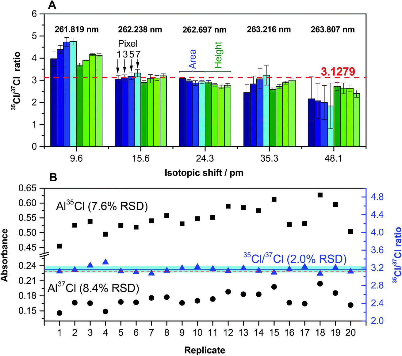Fig. 3 (A) Quantification of the Cl ratio for a solution (200 ng Cl) of CRM NIST 975a (35/37 = 3.1279 ± 0.0047) for different AlCl transitions. Values in blue were obtained using peak area, and values in green were obtained using peak height. In both cases, a lighter color intensity indicates a higher number of detector pixels (1, 3, 5 or 7). Error bars represent the standard deviation (n = 5). (B) Peak height values of 20 replicates of the same solution obtained for 262.222 (Al³⁷Cl) and 262.238 (Al³⁵Cl) nm transitions (left y-axis), and Cl ratios calculated from the same set of data (right y-axis). The red dashed line indicates the certified value. The blue line and the blue interval surrounding it represent the average value of the 20 replicates and its standard deviation, respectively. Reproduced with permission from the Royal Society of Chemistry (https://pubs.rsc.org/en/content/articlehtml/2015/ja/c5ja00055f).⁵⁴

Under optimized conditions, it is possible to carry out the isotopic analysis of Cl in 20 mg L⁻¹ solutions with precision values around 2% RSD (see Fig. 3B), without the need for any mass bias correction. This precision is not sufficient to monitor Cl isotopic natural variations, but it may be enough if the goal is to carry out tracer experiments, or to be able to calibrate by means of isotope dilution (ID). In fact, it was demonstrated in this work via analyses of natural water CRMs and well as commercially available mineral water samples that the use of ID serves to correct for interferences caused by chemical reactions (e.g., presence of high levels of Ca, thus leading to some Cl forming CaCl and not AlCl), as these interferences should affect both isotopes in practically the same way. This is one important conclusion of the work, as in GFMAS the occurrence of interferences of chemical origin is more common than in GFAAS.

A subsequent study by the same authors showed the potential of HR CS GFMAS for isotopic analysis of Br, using the CaBr molecule, after evaluating some alternative ones (such as AlBr and BaBr). In that case, the spectrum obtained was richer in lines, and there were several lines that responded selectively to the presence of Ca⁷⁹Br and Ca⁸¹Br. Interestingly, there were other lines in which both Ca⁷⁹Br and Ca⁸¹Br transitions overlapped, so they could be used for determining total Br content with higher signals.

The precision obtained for Br solutions of 10 mg L⁻¹ was 2.6%. Again, this is not sufficient for monitoring natural variations in Br isotopic composition. However, it was demonstrated that it is feasible to directly determine Br in solid samples despite the presence of interferences of chemical origin (e.g., very high Cl levels, which decrease the formation of CaBr due to the formation of CaCl instead⁵³) using ID for calibration. Fig. 4 shows the spectrum of a solid biological (tomato leaves) reference material vaporized together with a liquid spike. The peak profiles obtained are well-defined and unimodal, indicating that proper isotopic equilibration between the Br present in the solid and in the spike solution has occurred during the development of the temperature program, thus enabling ID to work properly.

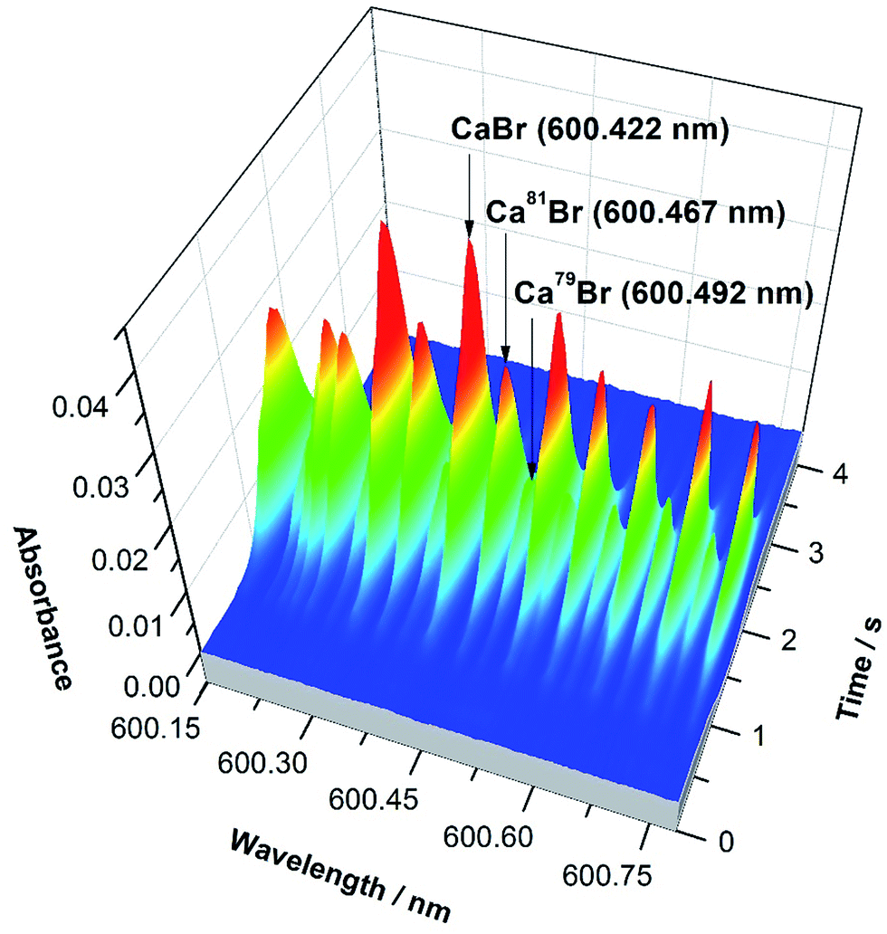Fig. 4 CaBr 3-D spectrum observed in the region of 600.4 nm when using HR CS GFMAS for the direct vaporization of a solid sample (SRM NIST 1573a tomato leaves) containing approximately 1.0 μg Br, mixed with a spike enriched in ⁸¹Br. The main band heads are highlighted. Reproduced with permission from the Royal Society of Chemistry https://pubs.rsc.org/en/content/articlehtml/2016/JA/C6JA00114A.⁵⁵

The last study reporting on this approach has been published by Abad et al.⁶⁷ In this work, B is the analyte, but instead of monitoring B atomic lines, BH was formed and measured via HR CS GFMAS. The expected difficulties for B vaporization discussed before were circumvented by a mixture of liquid and gas phase modifiers: a CaCl₂ solution with the aim to minimize the level of oxygen in the furnace and decrease the formation of boron carbide; a mannitol solution to prevent the formation of volatile boron species; X-100 triton as a surfactant; 2% CHF₃ in Ar to minimize memory effects; and 2% H₂ in Ar as a primary gas.

Two different portions of the spectrum were measured, in the vicinity of 433 nm and in the vicinity of 437 nm, both of them showing several lines, of which some were completely resolved for ¹⁰BH and ¹¹BH in the latter spectral region. The method finally developed was not very sensitive, requiring at least 1 g L⁻¹ of B. However, by using partial least regression and building a library of BH molecular spectra by monitoring solutions with different ¹¹B fractions, it was possible to report precisions in the range between 0.013 and 0.05%, which may suffice for monitoring B isotopic natural variations.

4.2. Nanoparticle characterization

HR CS AAS offers some possibilities for research in the nano field. In the beginning, some early studies were focused on the analysis of nanomaterials such as carbon nanotubes,²⁸ or the determination of nanoparticles (NPs) in tissues.⁶⁸ These studies, while relevant as applications, did not represent much of a change in the working procedure in comparison with analysis of other samples or other analytes. In other words, carrying out the direct analysis of impurities in carbon nanotubes is not so different from performing the direct analysis of impurities in other hard-to-dissolve carbonaceous materials, such as graphite. And those early studies aiming at the determination of NPs were, in fact, determining only the total elemental content, which was the result of exposure to NPs.

This situation has recently changed. It has been reported that it is feasible to obtain information on whether a particular element is found in the form of nanoparticles or in ionic form, and it may even be possible to calculate its size, when present as nanoparticles, all of this using GFAAS.

The first article to report on this aspect was published by Gagné et al.⁶⁹ It was demonstrated for Ag that atomization of nanoparticles requires more energy, and thus higher atomization temperatures, than the atomization of ionic species. And the greater the particle size, the higher the temperature required. Thus, they proposed the approach of either determining the atomization temperature or monitoring the changes in absorbance at different atomization temperatures, to detect the presence of AgNPs in biological samples (after sample preparation) and to have a rough estimation of their size.

This pioneering work did not make use of HR CS GFAAS but of line source GFAAS. However, there is an important reason for using HR GFAAS in that type of study, and that is the expanded possibility to directly analyze solid samples and complex materials in general.²¹ That is an intriguing aspect since many of the techniques that can be used for quantifying both the total content and the size distribution of nanoparticles, such as the increasingly popular single particle (SP)-ICP-MS, while offering several advantages, do not allow direct analysis of the samples. This could be an important issue because, as in every speciation/fractionation study, ensuring the preservation of the exact way in which the analyte is originally found in the sample during sample preparation is not trivial.

The next papers on this topic explored this possibility. In a first study, Feichtmeier and Leopold⁷⁰ showed the potential of SS HR CS GFAAS for the direct detection of Ag nanoparticles in parsley samples. They evaluated two different parameters, the so-called atomization delay (the time period between the beginning of the atomization step and the appearance of the peak maximum) and the atomization rate (the slope of a polynomial fitted curve calculated at the first inflection point of the absorbance vs. time peak profile). In the end, they proposed an approach based on both aspects. It is possible to assess if Ag is present in ionic form or as NPs simply by calculating this atomization delay (normalized to the sample mass): a difference of 6.27 ± 0.96 s mg⁻¹ between parsley samples containing ionic silver and AgNPs was found under optimum conditions. Furthermore, if AgNPs were found, the determination of the atomization rate permitted differentiation between NPs of 20, 60 and 80 nm.

A second study expanded the applicability of this method to different types of biological samples (namely parsley, apple, pepper, cheese, onion, pasta, maize meal, and wheat flour).⁷¹ This work focused on the use of the atomization delay to establish the presence of either ionic silver or AgNPs of 20 nm. It was found that the matrix plays an important role in the values found but, nevertheless, significant differences in this parameter between samples exposed to ionic silver or to AgNPs were observed in all cases investigated.

It is important to stress that this type of research abandons some of the classical GFAAS paradigms. In fact, the whole concept of stabilized temperature platform furnace (STPF) tries to minimize any potential difference in the signals obtained for the analyte, even when it could be present in various forms in the sample. In this particular case, the goal is exactly the opposite, and thus the conditions selected must be chosen with the aim of exacerbating the differences between the vaporization/atomization mechanisms of every species.

The work by Resano et al.⁷² showed that HR CS GFAAS could be applied to other NPs beside Ag, which was the focus of the previous studies. Also, the use of different parameters to quantify the presence and the size of NPs was discussed, and it was concluded that the time of appearance of the peak maximum was the preferred one in this case, as it did not depend on the concentration and permitted appreciation of clear differences according to the particle size, as shown in Fig. 5. It can also be appreciated in this figure that, under the conditions used (no modifier added and a very slow atomization ramp (150 °C s⁻¹)), the signal profiles observed for ionic Au and AuNPs were dissimilar: in the case of AuNPs, the signal is not only delayed according to its size, but its shape is practically Gaussian; on the other hand, the signals obtained for ionic Au show much more tailing, to the point that a secondary, smaller peak is found. This fact not only hints at different atomization mechanisms, but permits easy screening of the presence of either NPs or ions from an unknown solution.

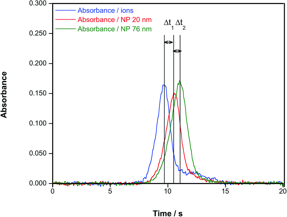Fig. 5 Time-resolved absorbance for a Au aqueous standard and for aqueous suspensions of AuNPs of 20 nm (diameter 19.6 nm; standard deviation: 2.1 nm, as estimated via TEM by the manufacturer) and 76 nm (diameter 75.7; standard deviation: 10.1 nm), respectively. In all cases, a concentration of 50 μg L⁻¹, an atomization temperature of 2000 °C and a heating ramp of 150 °C s⁻¹ were used. Reproduced with permission from the Royal Society of Chemistry https://pubs.rsc.org/en/Content/ArticleLanding/2016/JA/C6JA00280C.⁷²

Further work has basically confirmed the potential of the technique for sizing Au⁷³ and Au and Ag NPs,⁷⁴ respectively, despite some differences in the programs used by the different authors, and in the relation found between size and time of appearance (completely linear or not). Finally, another study demonstrated⁷⁵ the potential of solid sampling HR CS GFAAS for determining both the total Fe content (via measurement of the peak area) and the particle size (via evaluation of the atomization rate) in solid magnetic NPs.

Overall, this seems to be a relevant and growing field, where GFAAS can provide at least complementary information to other techniques. So far it cannot provide the same type of information as SP-ICP-MS, where not only the mean particle size but also the whole number-size distribution is obtained. But, as discussed before, the GFAAS capability to directly analyze complex samples is very interesting, and so is its ability to detect very small NPs (below 10 nm), which are not easily detected via SP-ICP-MS.

Still, more work is needed in order (i) to develop a more unified methodology and even terminology; (ii) to further improve the selectivity of the technique, as right now it is difficult to resolve mixtures of NPs or NPs with ionic species, requiring the use of deconvolution approaches,^72,73 or of previous separations (in this regard, cloud point extraction has been reported to enable the selective quantification of AgNPs and total Ag in waters with a LOD of 2 ng L⁻¹ using HR CS GFAAS⁷⁶); and (iii) to demonstrate the applicability of this approach to other types of NPs.

4.3. New instrumental developments

Perhaps the most critical aspect to move forward the application of HR CS AAS/MAS would be enhancing its multi-element capabilities.

In fact, one of the main historical motivations for the development of CS AAS was the possibility to implement higher multi-element capabilities, and when HR CS AAS instrumentation was made commercially available there were great expectations in this regard. It is necessary to state, however, that the potential of such commercial instrumentation to carry out the truly simultaneous monitoring of lines corresponding to different elements is rather limited.

The reason is simple and it is related with the optics and the detector capabilities: besides the optical system, in order to cover the whole UV-vis range with the resolution required (pm level), use of megapixel array detectors with a sufficiently fast response for transient signals would be required. Instead, the current instrument possesses a detector with only 588 pixels, but most of those are used for corrections, and only 200 are used to monitor the analytical signals. That is why the current instrumentation can measure simultaneously only a very small portion of the spectrum (0.2–1.0 nm, depending on the wavelength) with the required resolution.

The limitations of this instrumentation and the possibilities for multi-line monitoring are discussed in detail in previous studies,^18,19 so they will not be repeated herein. Also, a paper discussing the evolution of CS AAS, with an emphasis on detector requirements, was published by Becker-Ross et al.⁷⁷

It suffices to say that, at this point, with the commercially available instrumentation it is in principle possible to determine simultaneously several elements (a paper in which Co, Fe, Ni, and Pb were determined in solid samples has been reported²⁸), but this is more the exception than the rule, and most papers determine only one element and, in a few cases, two. It is also important to stress that this limitation is more relevant for GFAAS than for flame AAS, because in the latter case a fast sequential method may be sufficient in most practical situations, and the current instrumentation already enables this approach.²²

The important point regarding this aspect is that several recent studies demonstrate that it is technically possible to monitor a much wider portion of the spectrum simultaneously while still keeping the resolution required, which is always key (monitoring the whole UV-vis range with low resolution is not challenging at this point, but this approach is hardly suitable for analysis of complex samples⁷⁸). In order to do that, Geisler et al. proposed the use of a laser-driven xenon lamp as a continuum source, a CCD detector, and a modular simultaneous echelle spectrograph (MOSES).⁷⁹

A scheme of such instrumentation is shown in Fig. 6. This instrument can be operated in two modes (panorama or zoom), the former providing a wider spectral interval, and the latter higher resolution to focus on particular lines. Practically the whole UV spectrum (from 193 nm to 390 nm) can be covered with this instrument in four sub-areas (tiles): from 193.24 to 211.21 nm; from 209.83 to 236.00 nm; from 234.37 to 280.69 nm; and from 278.47 to 389.89 nm. These are the spectral windows that can be simultaneously monitored. Fig. 7 shows an example of all the elemental and molecular lines that can be seen using the last tile. This obviously represents a significant step forward in terms of multi-element possibilities. Again, as discussed in Section 3.1, it is worth stressing that this instrumentation offers the intriguing possibility of making simultaneous use of two techniques, AAS and MAS.

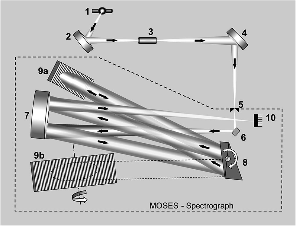Fig. 6 Schematic diagram of the experimental set-up including a MOSES spectrograph: (1) laser-driven continuum source, (2 and 4) transfer optics consisting of two elliptical mirrors, (3) atomizer, (5) entrance slit, (6) folding mirror, (7) off-axis parabolic mirror, (8) prism stage with two Littrow prisms, (9a and 9b) echelle gratings, and (10) CCD array detector. Reproduced with permission from Elsevier (https://www.sciencedirect.com/science/article/pii/S0584854715000543).⁷⁹

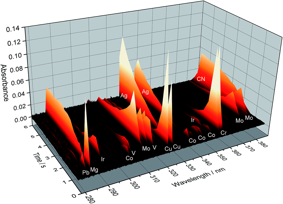Fig. 7 Temporally and spectrally resolved simultaneous multi-element absorption signals obtained by the MOSES spectrograph in the tile no. 4 setup, as obtained for 20 μL of a standard solution containing 50 μg L⁻¹ Cr and Cu; 100 μg L⁻¹ Co; 200 μg L⁻¹ As, Mo, Se, and V; and 2000 μg L⁻¹ Ir. Reproduced with permission from Elsevier (https://www.sciencedirect.com/science/article/pii/S0584854715000543).⁷⁹

In a second article of the same research group, this instrumentation was used to evaluate complete spectra of different diatomic molecules that can be used for S determination via HR CS GFMAS.⁴⁴ These molecules are GeS, SiS, SnS, and PbS, and the authors report the benefits of choosing GeS over the most popular today, CS, as it provides a (very slightly) lower characteristic mass (9.4 ng for GeS vs. 12 ng for CS using their most sensitive transitions) and its generation can be adjusted by controlling the Ge amount. Certainly, use of this type of instrument is beneficial to help in selecting the best transitions when molecular spectra very rich in lines are investigated.

Also, the possibility to monitor P₂ when aiming at P determination was investigated by Huang et al.⁸⁰ using a MOSES. The main advantage of selecting this molecule, in comparison with the measurement of P atomic absorption, is that it shows thousands of sharp transitions in the range between 196 and 245 nm that could be measured simultaneously and summed, in order to provide a better LOD,⁸¹ in addition to the much more gentle temperature program required.

Finally, the most recent work of this research group features the use of a MOSES to investigate CaF spectra,⁸² and also the use of minitubes of only 2 mm diameter to increase the sensitivity (an approach evaluated in a previous study⁸³) and of an autosampler capable of delivering volumes down to 30 nL. In this way, determination of F in sweat samples (12 to 49 mg L⁻¹) from cancer patients with volumes below 1 μL was achieved. The possibilities of this approach for situations in which sample volume is scarce or precious are therefore remarkable.

5. Conclusions

HR CS AAS/MAS is at a crossroads. It is no longer a young technique, but still too young to be considered as fully matured. While many of the research articles published provide a sense of continuity and a trend towards more applied work, there are also some promising novel areas, such as characterization of NPs or isotopic analysis, and a need for more fundamental studies, particularly in the case of HR CS MAS.

However, the final fate of the technique may well be related to the development of instrumentation commercially available with more multi-element potential, which seems possible from a technical point of view. It is however uncertain when (and if) this will happen. The fact that to this day only a manufacturer produces HR CS AAS/MAS instrumentation can be regarded as a drawback because, in principle, more competition should favor the development of new instrumental devices and also affect the price of acquisition of such instruments.

Conflicts of interest

There are no conflicts to declare.

Acknowledgements

The authors acknowledge funding from CTQ2015-64684-P (MINECO/FEDER) and from the Aragon Government (Grupo E43_17R, Fondo Europeo de Desarrollo Regional, Construyendo Europa desde Aragón).

References

1. B. Welz, H. Becker-Ross, S. Florek and U. Heitmann, High-resolution Continuum Source AAS. The Better Way to Do Atomic Absorption Spectrometry, Wiley-VCH, Weinheim, 2005.
2. B. Welz, F. G. Lepri, R. G. O. Araujo, S. L. C. Ferreira, M. D. Huang, M. Okruss and H. Becker-Ross, Anal. Chim. Acta, 2009, 647, 137–148.
3. D. J. Butcher, Anal. Chim. Acta, 2013, 804, 1–15.
4. M. Resano, M. R. Flórez and E. García-Ruiz, Anal. Bioanal. Chem., 2014, 406, 2239–2259.
5. P. N. Keliher and C. C. Wohlers, Anal. Chem., 1974, 46, 682–687.
6. A. T. Zander, T. C. O'Haver and P. N. Keliher, Anal. Chem., 1976, 48, 1166–1175.
7. B. T. Jones, B. W. Smith and J. D. Winefordner, Anal. Chem., 1989, 61, 1670–1674.
8. J. B. True, R. H. Williams and M. B. Denton, Appl. Spectrosc., 1999, 53, 1102–1110.
9. J. Harnly, J. Anal. At. Spectrom., 1999, 14, 137–146.
10. H. Becker-Ross, S. Florek, U. Heitmann and R. Weisse, Fresenius. J. Anal. Chem., 1996, 355, 300–303.
11. H. Becker-Ross and S. V. Florek, Spectrochim. Acta, Part B, 1997, 52, 1367–1375.
12. H. Becker-Ross, S. Florek and U. Heitmann, J. Anal. At. Spectrom., 2000, 15, 137–141.
13. B. Welz, Anal. Bioanal. Chem., 2005, 381, 69–71.
14. B. Welz, D. L. G. Borges, F. G. Lepri, M. G. R. Vale and U. Heitmann, Spectrochim. Acta, Part B, 2007, 62, 873–883.
15. B. Welz, M. G. R. Vale, D. L. G. Borges and U. Heitmann, Anal. Bioanal. Chem., 2007, 389, 2085–2095.
16. B. Welz, S. Morés, E. Carasek, M. G. R. Vale, M. Okruss and H. Becker-Ross, Appl. Spectrosc. Rev., 2010, 45, 327–354.
17. M. Resano and E. García-Ruiz, Anal. Bioanal. Chem., 2011, 399, 323–330.
18. M. Resano, L. Rello, M. Flórez and M. A. Belarra, Spectrochim. Acta, Part B, 2011, 66, 321–328.
19. M. Resano, M. R. Flórez and E. García-Ruiz, Spectrochim. Acta, Part B, 2013, 88, 85–97.
20. B. Welz, M. G. R. Vale, É. R. Pereira, I. N. B. Castilho and M. B. Dessuy, J. Braz. Chem. Soc., 2014, 25, 799–821.
21. M. Resano, M. Aramendía and M. A. Belarra, J. Anal. At. Spectrom., 2014, 29, 2229–2250.
22. C. C. Leite, A. de Jesus, M. L. Potes, M. A. Vieira, D. Samios and M. M. Silva, Energy Fuels, 2015, 29, 7358–7363.
23. M. Resano, F. Vanhaecke and M. T. C. De Loos-Vollebregt, J. Anal. At. Spectrom., 2008, 23, 1450–1475.
24. M. Resano, M. D. R. Flórez, I. Queralt and E. Marguí, Spectrochim. Acta, Part B, 2015, 105, 38–46.
25. S. de Oliveira Souza, L. L. François, A. R. Borges, M. G. R. Vale and R. G. O. Araujo, Spectrochim. Acta, Part B, 2015, 114, 58–64.
26. M. A. Bechlin, A. I. Barros, D. V. Babos, E. C. Ferreira and J. A. Gomes Neto, At. Spectrosc., 2017, 38, 62–67.
27. G. Dravecz, L. Bencs, D. Beke and Á. Gali, Talanta, 2016, 147, 271–275.
28. M. Resano, E. Bolea-Fernández, E. Mozas, M. R. Flórez, P. Grinberg and R. E. Sturgeon, J. Anal. At. Spectrom., 2013, 28, 657–665.
29. W. Boschetti, M. Orlando, M. Dullius, M. B. Dessuy, M. G. Vale, B. Welz and J. B. de Andrade, J. Anal. At. Spectrom., 2016, 31, 1269–1277.
30. M. Aramendía, M. R. Flórez, M. Piette, F. Vanhaecke and M. Resano, J. Anal. At. Spectrom., 2011, 26, 1964–1973.
31. D. V. de Babos, M. A. Bechlin, A. I. Barros, E. C. Ferreira, J. A. Gomes Neto and S. R. de Oliveira, Talanta, 2016, 152, 457–462.
32. R. Dobrowolski, A. Mróz, M. Dąbrowska and P. Olszański, Spectrochim. Acta, Part B, 2017, 132, 13–18.
33. I. López García, S. Rengevicova, M. J. Muñoz-Sandoval and M. Hernández-Córdoba, Talanta, 2017, 162, 309–315.
34. I. López García, M. J. Muñoz-Sandoval and M. Hernández-Córdoba, Talanta, 2017, 172, 8–14.
35. M. Aramendía, A. Guarda, D. Leite and M. Resano, J. Anal. At. Spectrom., 2017, 32, 2352–2359.
36. L. Colares, É. R. Pereira, J. Merib, J. C. Silva, J. M. Silva, B. Welz, E. Carasek and D. L. G. Borges, J. Anal. At. Spectrom., 2015, 30, 381–388.
37. N. L. A. Jamari, A. Behrens, A. Raab, E. Krupp and J. Feldmann, J. Anal. At. Spectrom., 2018, 33, 1304–1309.
38. U. Heitmann, H. Becker-Ross, S. Florek, M. D. Huang and M. Okruss, J. Anal. At. Spectrom., 2006, 21, 1314–1320.
39. H. Gleisner, B. Welz and J. W. Einax, Spectrochim. Acta, Part B, 2010, 65, 864–869.
40. H. Gleisner, J. W. Einax, S. Morés, B. Welz and E. Carasek, J. Pharm. Biomed. Anal., 2011, 54, 1040–1046.
41. I. Würtenberger and R. Gust, Anal. Bioanal. Chem., 2014, 406, 3431–3442.
42. Z. Qin, D. McNee, H. Gleisner, A. Raab, K. Kyeremeh, M. Jaspars, E. Krupp, H. Deng and J. Feldmann, Anal. Chem., 2012, 84, 6213–6219.
43. S. Morés, G. C. Monteiro, F. da Silva Santos, E. Carasek and B. Welz, Talanta, 2011, 85, 2681–2685.
44. M. D. Huang, H. Becker-Ross, S. Florek, C. Abad and M. Okruss, Spectrochim. Acta, Part B, 2017, 135, 15–21.
45. M. Dessuy, M. G. Vale, F. Lepri, B. Welz and U. Heitmann, Spectrochim. Acta, Part B, 2007, 62, 429–434.
46. F. G. Lepri, B. Welz, M. B. Dessuy, M. G. Vale, D. Bohrer, M. T. C. de Loos-Vollebregt, M. D. Huang and H. Becker-Ross, Spectrochim. Acta, Part B, 2010, 65, 24–32.
47. M. Resano, J. Briceño and M. A. Belarra, J. Anal. At. Spectrom., 2009, 24, 1343–1354.
48. M. D. Huang, H. Becker-Ross, S. Florek, U. Heitmann and M. Okruss, Spectrochim. Acta, Part B, 2006, 61, 959–964.
49. É. R. Pereira, B. Welz, A. H. D. Lopez, J. S. de Gois, G. F. Caramori, D. L. G. Borges, E. Carasek and J. B. de Andrade, Spectrochim. Acta, Part B, 2014, 102, 1–6.
50. A. Guarda, M. Aramendía, I. Andrés, E. García-Ruiz, P. C. do Nascimento and M. Resano, Talanta, 2017, 162, 354–361.
51. H. Tinas and S. Akman, Spectrochim. Acta, Part B, 2018, 148, 60–64.
52. R. L. da S Medeiros, S. O. Souza, R. G. O. Araujo, D. R. da Silva and T. de A Maranhão, Talanta, 2018, 176, 227–233.
53. M. R. Flórez and M. Resano, Spectrochim. Acta, Part B, 2013, 88, 32–39.
54. F. V. Nakadi, M. A. M. S. da Veiga, M. Aramendía, E. García-Ruiz and M. Resano, J. Anal. At. Spectrom., 2015, 30, 1531–1540.
55. F. V. Nakadi, M. A. M. S. da Veiga, M. Aramendía, E. García-Ruiz and M. Resano, J. Anal. At. Spectrom., 2016, 31, 1381–1390.
56. F. Čacho, Ľ. Machyňák, M. Němeček and E. Beinrohr, Spectrochim. Acta, Part B, 2018, 144, 63–67.
57. M. B. T. Zanatta, F. V. Nakadi and M. A. M. S. da Veiga, Talanta, 2018, 179, 563–568.
58. N. Ozbek and S. Akman, J. Anal. At. Spectrom., 2018, 33, 111–117.
59. J. Acker, S. Bücker and V. Hoffmann, J. Anal. At. Spectrom., 2016, 31, 902–911.
60. L. F. C. Gouvêa, A. J. Moreira, C. D. Freschi and G. P. G. Freschi, J. Food Compost. Anal., 2018, 70, 28–34.
61. M. L. Oliveira, G. C. Brandao, J. B. de Andrade and S. L. C. Ferreira, Talanta, 2018, 179, 810–815.
62. H. Wiltsche, K. Prattes, M. Zischka and G. Knapp, Spectrochim. Acta, Part B, 2009, 64, 341–346.
63. M. Resano, J. Briceño, M. Aramendía and M. A. Belarra, Anal. Chim. Acta, 2007, 582, 214–222.
64. R. E. Russo, A. A. Bol'shakov, X. Mao, C. P. McKay, D. L. Perry and O. Sorkhabi, Spectrochim. Acta, Part B, 2011, 66, 99–104.
65. A. A. Bol'shakov, X. Mao, J. J. Gonzalez and R. E. Russo, J. Anal. At. Spectrom., 2016, 31, 119–134.
66. G. Herzberg, Molecular Spectra and Molecule Structure. Diatomic Molecules, D. Van Nostrand, 2nd edn, 1950.
67. C. Abad, S. Florek, H. Becker-Ross, M. D. Huang, H.-J. Heinrich, S. Recknagel, J. Vogl, N. Jakubowski and U. Panne, Spectrochim. Acta, Part B, 2017, 136, 116–122.
68. M. Resano, E. Mozas, C. Crespo, J. Briceño, J. Del Campo Menoyo and M. A. Belarra, J. Anal. At. Spectrom., 2010, 25, 1864–1873.
69. F. Gagné, P. Turcotte and C. Gagnon, Anal. Bioanal. Chem., 2012, 404, 2067–2072.
70. N. S. Feichtmeier and K. Leopold, Anal. Bioanal. Chem., 2014, 406, 3887–3894.
71. N. S. Feichtmeier, N. Ruchter, S. Zimmermann, B. Sures and K. Leopold, Anal. Bioanal. Chem., 2016, 408, 295–305.
72. M. Resano, E. García-Ruiz and R. Garde, J. Anal. At. Spectrom., 2016, 31, 2233–2241.
73. K. Leopold, A. Brandt and H. Tarren, J. Anal. At. Spectrom., 2017, 32, 723–730.
74. T. Panyabut, N. Sirirat and A. Siripinyanond, Anal. Chim. Acta, 2018, 1000, 75–84.
75. M. M. L. Guerrero, M. T. S. Cordero, E. V. Alonso, J. M. C. Pavón and A. García de Torres, J. Anal. At. Spectrom., 2015, 30, 1169–1178.
76. I. López-García, Y. Vicente-Martínez and M. Hernández-Córdoba, Spectrochim. Acta, Part B, 2014, 101, 93–97.
77. H. Becker-Ross, S. Florek, U. Heitmann, M. Huang, M. Okruss and B. Radziuk, Spectrochim. Acta, Part B, 2006, 61, 1015–1030.
78. D. Katskov, Spectrochim. Acta, Part B, 2015, 105, 25–37.
79. S. Geisler, M. Okruss, H. Becker-Ross, M. D. Huang, N. Esser and S. Florek, Spectrochim. Acta, Part B, 2015, 107, 11–16.
80. M. D. Huang, H. Becker-Ross, M. Okruss, S. Geisler and S. Florek, Spectrochim. Acta, Part B, 2016, 115, 23–30.
81. U. Heitmann, B. Welz, D. Borges and F. Lepri, Spectrochim. Acta, Part B, 2007, 62, 1222–1230.
82. Y. Xing, H. Fuss, J. Lademann, M. D. Huang, H. Becker-Ross, S. Florek, A. Patzelt, M. C. Meinke, S. Jung and N. Esser, Spectrochim. Acta, Part B, 2018, 142, 91–96.
83. M. D. Huang, H. Becker-Ross, M. Okruss, S. Geisler and S. Florek, J. Anal. At. Spectrom., 2012, 27, 982–988.
84. A. V. Zmozinski, T. Llorente-Mirandes, I. C. F. Damin, J. F. López-Sánchez, M. G. R. Vale, B. Welz and M. M. Silva, Talanta, 2015, 134, 224–231.
85. M. Schneider, H. R. Cadorim, B. Welz, E. Carasek and J. Feldmann, Talanta, 2018, 188, 722–728.
86. A. M. Orani, E. Han, P. Mandjukov and E. Vassileva, Spectrochim. Acta, Part B, 2015, 103–104, 131–143.
87. A. M. Orani, P. Mandjukov and E. Vassileva, Int. J. Environ. Anal. Chem., 2017, 97, 710–729.
88. A. I. Barros, K. Miranda, E. C. Ferreira and J. A. Gomes Neto, At. Spectrosc., 2015, 36, 102–107.
89. H. Tinas, N. Ozbek and S. Akman, Microchem. J., 2018, 138, 316–320.
90. A. V. Zmozinski, T. Pretto, A. R. Borges and M. G. R. Vale, Anal. Methods, 2015, 7, 3735–3741.
91. A. R. Borges, D. N. Bazanella, Á. T. Duarte, A. V. Zmozinski, M. G. R. Vale and B. Welz, Microchem. J., 2017, 130, 116–121.
92. M. Pozzatti, A. R. Borges, M. B. Dessuy, M. G. R. Vale and B. Welz, Anal. Methods, 2017, 9, 329–337.
93. A. Virgilio, J. F. Rêgo, A. I. Barros and J. A. Gomes Neto, J. Braz. Chem. Soc., 2015, 26, 1988–1993.
94. D. V. L. Ávila, A. R. Borges, M. G. R. Vale, R. G. O. Araujo and E. A. Passos, Microchem. J., 2017, 133, 524–529.
95. D. V. Babos, A. I. Barros, E. C. Ferreira and J. A. Gomes Neto, Spectrochim. Acta, Part B, 2017, 130, 39–44.
96. A. S. Silva, G. C. Brandao, G. D. Matos and S. L. C. Ferreira, Talanta, 2015, 144, 39–43.
97. E. G. Barrera, D. Bazanella, P. W. Castro and W. Boschetti, Microchem. J., 2017, 132, 365–370.
98. A. S. dos Passos, G. F. Tonon, F. V. Nakadi, A. S. Mangrich, J. B. de Andrade, B. Welz and M. G. R. Vale, Anal. Methods, 2018, 10, 3645–3653.
99. A. V. Zmozinski, T. Pretto, A. R. Borges, A. T. Duarte and M. G. R. Vale, Microchem. J., 2016, 128, 89–94.
100. A. R. Borges, L. L. François, E. M. Becker, M. G. R. Vale and B. Welz, Microchem. J., 2015, 119, 169–175.
101. Z. Ajtony, N. Laczai, G. Dravecz, N. Szoboszlai, Á. Marosi, B. Marlok, C. Streli and L. Bencs, Food Chem., 2016, 213, 799–805.
102. L. O. dos Santos, G. C. Brandao, A. M. P. dos Santos, S. L. C. Ferreira and V. A. Lemos, Food Anal. Method., 2017, 10, 469–476.
103. R. R. Gamela, A. T. Duarte, E. G. Barrera, B. Welz, M. B. Dessuy, M. M. da Silva and M. G. R. Vale, Anal. Methods, 2017, 9, 2321–2327.
104. E. Vereda Alonso, M. López Guerrero, M. Siles Cordero, J. M. Cano Pavón and A. García de Torres, J. Anal. At. Spectrom., 2016, 31, 2391–2398.
105. B. M. Soares, R. F. Santos, R. C. Bolzan, E. I. Muller, E. G. Primel and F. A. Duarte, Talanta, 2016, 160, 454–460.
106. M. Pozzatti, F. V. Nakadi, M. G. R. Vale and B. Welz, Microchem. J., 2017, 133, 162–167.
107. A. C. Valdivia, E. V. Alonso, M. M. L. Guerrero, J. Gonzalez-Rodriguez, J. M. C. Pavón and A. García de Torres, Talanta, 2018, 179, 1–8.
108. P. Mandjukov, A. M. Orani, E. Han and E. Vassileva, Spectrochim. Acta, Part B, 2015, 103–104, 24–33.
109. A. Baysal and S. Akman, Anal. Lett., 2016, 49, 1896–1902.
110. N. Laczai, L. Kovács, Á. Péter and L. Bencs, Spectrochim. Acta, Part B, 2016, 117, 8–15.
111. G. Dravecz, N. Laczai, I. Hajdara and L. Bencs, Spectrochim. Acta, Part B, 2016, 126, 1–5.
112. R. M. Andrade, J. S. Gois, I. M. Toaldo, D. B. Batista, A. S. Luna and D. L. G. Borges, Food Anal. Method., 2017, 10, 1209–1215.
113. J. S. de Gois, T. S. Almeida, R. M. de Andrade, I. M. Toaldo, M. T. Bordignon-Luiz and D. L. G. Borges, Microchem. J., 2016, 124, 283–289.
114. S. Kelestemur and M. Özcan, Microchem. J., 2015, 118, 55–61.
115. A. I. Barros, T. V. Silva, E. C. Ferreira and J. A. Gomes Neto, J. Braz. Chem. Soc., 2015, 26, 140–146.
116. T. V. Silva, K. Miranda, E. C. Ferreira, M. C. Santos, J. A. Gomes Neto and F. Barbosa, At. Spectrosc., 2015, 36, 182–186.
117. N. Ozbek, S. Ustabası and S. Akman, J. Anal. At. Spectrom., 2015, 30, 1782–1786.
118. L. Rello, M. Aramendía, M. A. Belarra and M. Resano, Bioanalysis, 2015, 7, 2057–2070.
119. A. T. Duarte, A. R. Borges, A. V. Zmozinski, M. B. Dessuy, B. Welz, J. B. de Andrade and M. G. R. Vale, Talanta, 2016, 146, 166–174.
120. J. Coco, M. A. Bechlin, A. I. Barros, E. C. Ferreira, M. A. M. S. Veiga and J. A. Gomes Neto, At. Spectrosc., 2017, 38, 208–212.
121. S. S. Fick, F. V. Nakadi, F. Fujiwara, P. Smichowski, M. G. R. Vale, B. Welz and J. B. de Andrade, J. Anal. At. Spectrom., 2018, 33, 593–602.
122. E. Zambrzycka-Szelewa, M. Lulewicz and B. Godlewska-Żyłkiewicz, Spectrochim. Acta, Part B, 2017, 133, 81–87.
123. A. I. Barros, D. V. de Babos, E. C. Ferreira and J. A. Gomes Neto, Talanta, 2016, 161, 547–553.
124. W. Boschetti, L. M. G. Dalagnol, M. Dullius, A. V. Zmozinski, E. M. Becker, M. G. R. Vale and J. B. de Andrade, Microchem. J., 2016, 124, 380–385.
125. F. V. Nakadi, C. Prodanov, W. Boschetti, M. G. R. Vale, B. Welz and J. B. de Andrade, Talanta, 2018, 179, 828–835.
126. J. Patočka, L. Bendakovská, A. Krejčová, T. Černohorský, M. Resano and P. Bělina, Anal. Methods, 2017, 9, 705–715.
127. J. S. de Gois, É. R. Pereira, B. Welz and D. L. G. Borges, Spectrochim. Acta, Part B, 2017, 132, 50–55.
128. É. R. Pereira, L. M. Rocha, H. R. Cadorim, V. D. Silva, B. Welz, E. Carasek and J. B. de Andrade, Spectrochim. Acta, Part B, 2015, 114, 46–50.
129. M. S. P. Enders, A. O. Gomes, R. F. Oliveira, R. C. L. Guimarães, M. F. Mesko, E. M. de M. Flores and E. I. Muller, Energy Fuels, 2016, 30, 3637–3643.
130. Ľ. Machyňák, F. Čacho, M. Němeček and E. Beinrohr, Spectrochim. Acta, Part B, 2016, 125, 140–145.
131. N. Ozbek and S. Akman, J. Agric. Food Chem., 2016, 64, 5767–5772.
132. M. A. Bechlin, E. C. Ferreira and J. A. Gomes Neto, Microchem. J., 2017, 132, 130–135.
133. É. R. Pereira, J. Merib, H. R. Cadorim, M. Schneider, G. S. Carvalho, F. A. Duarte, B. Welz, J. del Campo Menoyo and J. Feldmann, Food Control, 2017, 78, 456–462.
134. I. K. S. Oliveira, R. L. S. Medeiros, D. R. Silva and T. A. Maranhão, J. Braz. Chem. Soc., 2018, 29, 571–578.
135. P. M. Machado, S. Morés, É. R. Pereira, B. Welz, E. Carasek and J. B. de Andrade, Spectrochim. Acta, Part B, 2015, 105, 18–24.
136. N. Ozbek and S. Akman, LWT--Food Sci. Technol., 2015, 61, 112–116.
137. A. R. Borges, A. T. Duarte, M. da L. Potes, M. M. Silva, M. G. R. Vale and B. Welz, Microchem. J., 2016, 124, 410–415.
138. N. Ozbek and S. Akman, Food Chem., 2016, 211, 180–184.
139. P. V. Zaitceva and A. A. Pupyshev, Analytics and Control, 2016, 20, 34–40.
140. N. Ozbek and S. Akman, Food Anal. Method., 2016, 9, 2925–2932.
141. J. S. de Gois, T. S. Almeida, J. C. Alves, R. G. O. Araujo and D. L. G. Borges, Environ. Sci. Technol., 2016, 50, 3031–3038.
142. N. Ozbek, H. Baltaci and A. Baysal, Environ. Sci. Pollut. Res., 2016, 23, 13169–13177.
143. W. Boschetti, M. B. Dessuy, A. H. Pizzato and M. G. R. Vale, Microchem. J., 2017, 130, 276–280.
144. M. Krawczyk-Coda and E. Stanisz, Anal. Bioanal. Chem., 2017, 409, 6439–6449.
145. P. Ley, M. Sturm, T. A. Ternes and B. Meermann, Anal. Bioanal. Chem., 2017, 409, 6949–6958.
146. Ľ. Machyňák, E. Beinrohr, M. Němeček and F. Čacho, Chem. Listy, 2017, 111, 663–666.
147. M. Němeček, Ľ. Machyňák, E. Beinrohr, F. Čacho and P. Horváth, Chem. Listy, 2017, 111, 588–590.
148. J. B. S. Espinelli Jr, D. G. V. Tinoco and R. Carapelli, Spectrochim. Acta, Part B, 2018, 149, 156–162.
149. Y. Wang, L. Zhong, T. Yang and Z. Y. Shi, Metall. Anal., 2016, 36, 1–5.
150. L. N. Pires, G. C. Brandao and L. S. G. Teixeira, Food Chem., 2017, 225, 162–166.
151. N. Ozbek and A. Baysal, Food Chem., 2015, 168, 460–463.
152. S. Gunduz and S. Akman, Food Chem., 2015, 172, 213–218.
153. C. S. Huber, M. G. R. Vale, B. Welz, J. B. Andrade and M. B. Dessuy, Spectrochim. Acta, Part B, 2015, 108, 68–74.
154. W. C. Zu, Y. Wang, Y. X. Zhang, B. N. Li, C. Liu and M. Ren, Spectrosc. Spectral Anal., 2016, 36, 1221–1224.
155. E. Andrade-Carpente, E. Peña-Vázquez and P. Bermejo-Barrera, Spectrochim. Acta, Part B, 2016, 122, 188–191.
156. N. Ozbek and S. Akman, Food Chem., 2016, 213, 529–533.
157. N. Ozbek and A. Baysal, Int. J. Environ. Anal. Chem., 2016, 96, 505–514.
158. H. R. Cadorim, É. R. Pereira, E. Carasek, B. Welz and J. B. de Andrade, Talanta, 2016, 146, 203–208.
159. N. Ozbek and A. Baysal, Spectrochim. Acta, Part B, 2017, 130, 17–20.
160. A. S. Camera, P. P. Arcênio, W. de Oliveira Pacheco Filho, T. de Andrade Maranhão, F. J. S. de Oliveira and V. L. A. Frescura, Microchem. J., 2017, 134, 301–308.
161. E. R. Pereira, B. Welz and A. A. Vieira, J. Anal. At. Spectrom., 2018, 33, 1394–1401.
162. J. S. Almeida, L. A. Meira and L. S. G. Texeira, Microchem. J., 2018, 143, 155–159.
163. Y. Arslan, J. A. C. Broekaert and I. Kula, Anal. Sci., 2018, 34, 831–836.

---