 Open Access Article
Creative Commons Attribution 3.0 Unported Licence
Efficient kinetic experiments in continuous flow microreactors
Kosi C.
Aroh
 and
Klavs F.
Jensen
 *
*
Department of Chemical Engineering, Massachusetts Institute of Technology, Cambridge, MA 02139, USA. E-mail: kfjensen@mit.edu
First published on 15th January 2018
Abstract
Flow chemistry is an enabling technology that can offer an automated and robust approach for the generation of reaction kinetics data. Recent studies have taken advantage of transient flows to quickly generate concentration profiles with various online analytical tools. In this work, we demonstrate an improved method where temperature and flow are transient throughout the reaction. It was observed that only two orthogonal temperature ramp experiments under the same transient flow condition were sufficient to characterize a Paal–Knorr (one step bimolecular) reaction within our chosen reaction space. This method further shortens the time and decreases the materials needed to collect sufficient kinetic data and provides a framework with which more complex kinetic studies could be performed.
Introduction
Knowledge of chemical reaction kinetics and corresponding mechanisms is important for the development of new reactions and optimization of reaction conditions for laboratory and industrial applications.1,2 With the increasing utility of machine learning, specifically in chemical synthetic route predictions, this information is evermore desired in order to enhance accuracy and usefulness of these predictions with more accurate data for model training.3–5 In addition, lower computational costs are moving the bottle neck of reaction engineering to the collection of experimental data. Flow-based microreactors have risen as a technology capable of addressing this issue amongst others. They provide the benefits of ease of process automation, higher heat and mass transfer rates and a more straightforward incorporation of inline analysis tools compared to traditional batch setups.6–11 Continuous flow systems have been used for complex chemical synthesis,12–15 gas-phase reactions,16–19 photochemistry,20–23 electrochemistry,24,25 and reaction optimization26–28 but their robustness for reaction kinetics is hindered by the need to take steady state measurements.29–32Recent studies have shown that transient flow data could be used to quickly generate kinetic data.33–36 Mozharov used the transient data generated from a step change in flow to scan different reaction times and fit kinetic data collected with inline Raman spectroscopy.33 However it was concluded that the method was limited since the procedure to extract kinetics was based on estimating when the transient flow started and stopped. Moore and Jensen improved the method by gradually increasing the flow rate, allowing for a more accurate tracking of reaction times, utilizing infrared spectroscopy.34 Schwolow et al.'s in situ Raman-equipped microreactor setup utilized this gradual flowrate change approach to quickly collect kinetics of Michael addition reaction.35 Hone et al. then applied this method to a multistep SNAr reaction in order to demonstrate its robustness for more complex mechanisms and the effect of dispersion in these systems.36
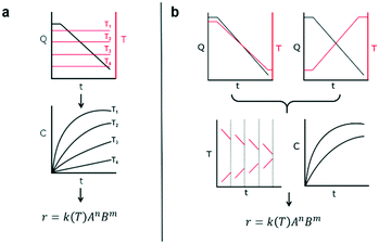
This work introduces a new approach that builds upon previously reported studies, resulting in a more efficient method for reaction kinetics. The approach, outlined in Fig. 1, involves simultaneously changing flow rates and temperature within one experiment. This contrasts to traditional methods where temperature is kept constant and several experiments are needed in order to understand how the reaction depends on both temperature and time. The advantage of this approach is that less time can be devoted to experimental setup and data collection and instead spent on data analysis which can be automated and more readily sped up. Though temperature ramps have been used in the past for kinetic studies, their application still remains limited.37 Furthermore, the idea of observing both temperature and residence time changes simultaneously have not been proposed largely due to the analytical complexity arising from the choice of experimental setup.
The philosophy behind this method also differs from the one suggested by Blackmond for mechanistic investigation of catalytic systems.38 In that approach, calorimetry measurements of reaction rate are used to infer reaction order given different starting conditions of reagents. In our approach, instead, an experiment that simultaneously covers all reaction conditions is performed and deconstructed later during data analysis. As mentioned earlier, the method involves changing the flowrate and temperature continuously throughout the course of the experiment. The shape of the temperature or resulting residence time profile that the user samples is not critical to the success of the approach as long as they sufficiently sample the reaction space. The idea of sufficient space sampling ramps has its basis in traditional design of experiments for which it is important to choose orthogonal experiments in order to account independently for effects of each variable (more on this later).
Method
Simultaneous residence and temperature ramps
The accuracy of this method requires a good understanding of the nonlinearities created by the transient flow and temperature profiles. Microreactors play a key role because they simplify the complexities that may arise in larger transient flow systems. The small length scale produces laminar flow. This results in a parabolic flow profile in the channels that, although becomes easier to model, could introduce dispersion into the system that could complicate data analysis.39 Specifically for our microreactor system, the dispersion has been calculated to only introduce a very small deviation from plug flow reactor conditions.31,36,39,40 In order to accurately observe a range of residence times within one experiment, from the derivation previously reported, a linear ramp in residence time can be generated from an exponential change in flowrate.34 | (1) |
 | (2) |
 | (3) |
For this work the two reagent equivalents were kept constant so their flow rates (Q1 and Q2) were simply half of the total. Changing the ratio of the reagents throughout an experiment is also a possibility and could serve as another parametric insight alongside the residence time. This was not attempted for this reaction since it was known beforehand that equivalents was not a major kinetic factor for the chosen reaction. At the exit of the reactor the inline analytical tool records the concentration and matches it to the correct residence time. The residence time corresponding to each measurement (τ) is a function of the following: the predefined rate of change of the instantaneous residence time (τins) versus time (α), reactor volume (Vr), dead volume between reactor exit and measurement point (Vd), time of measurement (tm), and residence time at start of ramp (τ0). The residence time is also defined by the time the fluid element enters (ti) and exits (tf) the reactor. This definition combined with eqn (2) for measurement time (tm) is used keep track of the temperature profile this fluid element experiences. The linear temperature ramp is simultaneously carried out according to eqn (4). Here b, the ramp rate, could be negative or positive depending on whether the temperature was being ramped down or up, respectively.
| T = T0 + bt | (4) |
Analysis procedure
The Paal–Knorr cyclocondensation reaction for the synthesis of pyrroles from 2,5-hexanedione (2) and ethanolamine (1) in DMSO (Scheme 1) was chosen for this study due to its simplicity and its well established usefulness for the synthesis of heterocycles.30 Previous mechanistic studies have shown the rate determining step to be the cyclization step and for that reason the reaction was assumed to follow a single step mechanism with an unknown pre-exponential parameter (A), temperature dependence term (‘activation energy’) (E) and reaction orders (m,n).41| r = kĈm1Ĉn2 |
The governing equation for the reactor is needed in order to extract the kinetics from the measured data. The mass transfer of species in the system is described by a second order nonlinear differential equation:
The small dispersion and small reactor channels relative to the reactor length allows us to ignore the second order term due to the large Peclet number. This then results in the familiar design equation for a plug flow reactor (pfr).
The equations for the other two species (ethanolamine and product) follow a similar procedure to give similar pfr design equations. These equations were used to simulate the concentration (Ĉ2) of hexanedione under various experimental conditions and compared to the experimental concentrations (C2) measured. The residence time of each measurement, determined by eqn (3). Eqn (4), was used to calculate the instantaneous temperature but the portion of the profile that the current fluid element, j, saw was determined by the following equation:
| Tj,o = To + b(tm − τj − tf) |
θ = [log![[thin space (1/6-em)]](https://www.rsc.org/images/entities/char_2009.gif) A,E/1000R,m,n] A,E/1000R,m,n] |
In summary, a ramp experiment produces a series of points. Each point measured during the experiment spent a known residence time in the reactor and experienced a series of temperatures. For each measured point the following equations for the measured concentration were solved using MATLAB's ode solver.
| T = Tj,o + bτ |
| T(0) = Tj,o, C1(0) = C2(0) = 0.5 M |
| τ = 0…τj |
Experimental method
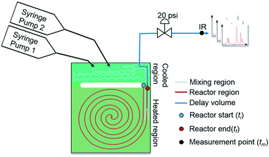
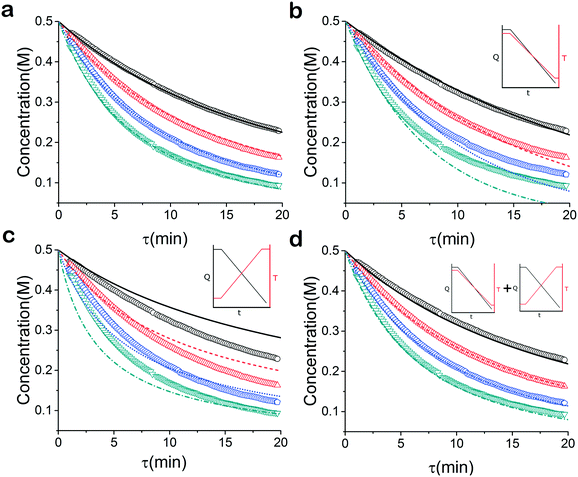
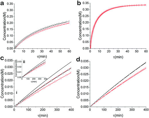
As mentioned earlier, microreactors allow for the controlled continuous flow rate and temperature change within a single experiment. A silicon microreactor, reported previously31,42 was used to carry out all experiments. The reactor had a mixing region and an outlet region that was cooled to 15 °C. A cartridge heater enclosed in an aluminium chuck heated the main reactor section. The experimental setup consisted of two syringe pumps that pushed reagents into a microreactor in which the mixing and reaction occurred (Fig. 2). A backpressure of 20 psi served to stabilize flow from the syringe pumps before it arrived at an infrared spectrometer equipped with a 10 μL flow cell (React IR IC 10). A LabVIEW and MATLAB program enabled the automation of all experiments. One equivalent of both reagents with an initial concentration of 0.5 M in the reactor was used for all experiments. The simulated experiments incorporated the correct temperature history of each measured point collected as described earlier. For the experiments mentioned here, a constant temperature ramp of 1 °C min−1 from 40 °C to 100 °C was applied. The temperature was held constant at the endpoint of the ramp. The residence time ramp was defined by a constant slope (α) of 0.4 when comparing the instantaneous residence time to experimental time. The experiments were initialized at a steady state residence time of half a minute before starting the ramps that went from 0.5 to 20 minutes. The linear temperature ramp up (EXP1) and down (EXP2) experiments were fitted individually and simultaneously (EXP1 + EXP2) and the results are shown in Fig. 3. Concentration profiles from residence time ramps at four different but constant temperatures (40 °C, 60 °C, 80 °C, 100 °C) were also collected to facilitate method validation (Fig. 4a).Results
Method validation
When analysed separately, the results from the temperature ramps experiments and model with fitted parameters (θup, θdown) were in very good agreement (Fig. 3a and b). While good agreement was observed for the simultaneous fitting (θu+d), there seems to be lack of fit at higher residence times (Fig. 3c). From this data alone, it is hard to tell how representative the regressed parameters are to the actual system since each experiment only looked at a small subset of the experimental space. This issue arises from the highly correlated nature of the parameters and the potential to over fit the experimental data.For this reason the produced models were compared to the data collected at four different temperatures to validate the accuracy of the proposed approach. Fig. 4a shows the experimental data and its corresponding first order model fitted parameters (θconst-T). The high coefficient of determination (R2) of 0.99 validates the current model assumption that a one step process correctly describes the consumption of the diketone in this Paal–Knorr reaction. In Fig. 4b–d, the parameters generated from the regressions in Fig. 4 are compared against the same constant temperature, residence time ramp data. An immediate observation is that the parameters (θu+d) from fitting the temperature ramps up and down simultaneously are in better agreement with the constant temperature data than the individually fitted parameters (θup, θdown) i.e. EXP1 + EXP2 > EXP1 or EXP2. Upon closer inspection, the individual results of θup and θdown match the constant temperature data at points that were “seen” in their respective experiments, but they fail to describe the reaction over the complete parameter space. This discrepancy could be a result of overfitting since the pre-exponential factor and temperature dependence term are highly correlated. A better explanation is that EXP1 or EXP2 by itself is not sufficient to decouple the effects of temperature and time. In one experiment, temperature is increasing with residence time with the measured concentration of 2,5-hexandione decreasing with time. By combining the two experiments we produced two orthogonal experiments that were sufficient to describe the reaction over the chosen experiment space.
Another observation and the main point of this work is that Fig. 4a and d produce similar results, i.e. both produce high coefficient of determination (∼0.99) when compared to the constant temperature ramps. Conceptually this means that the amount of information in the various temperature versus residence time plots is also present in the combined temperature ramp up and down experiment with the main difference being the time and material it takes to perform the two experiments. The constant temperature residence time ramps needed four experiments in this case in order to build the model while the combined temperature ramp up and down experiments only required two.
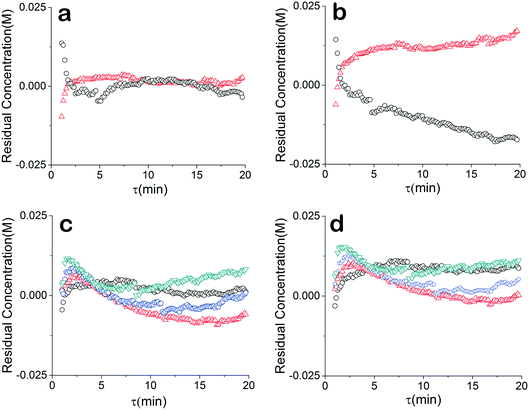
The residuals of our data were also compared to further understand the relationship between our chosen model and the data. For a good unbiased model, it is important that the residuals are randomly distributed around zero over the design space. The regressed model (θconst-T) from the constant temperature data fit the temperature ramp experiments very well (Fig. 5a and c). The higher residuals at low residence times is due to less accuracy of the approach stemming from higher reaction rate, faster flow rate and the sampling time of the IR. The sensitivity could be further addressed by decreasing the rate of transient changes and decreasing the IR sample time. On the other hand, a drift in the residuals from the temperature ramp model (θu+d) is observed (Fig. 5b), implying a model that does not fully capture the physics. Though, comparing the residuals of the two models concentration profiles at different constant temperatures does not show that information is missing from the models. Rather the results underscore the nonlinearity and correlated nature of parameters of kinetic rate constants since the discrepancy of the two models is only noticed in the temperature ramp results.
Instead of assuming that temperature played a major role in the difference, we explored whether better regression could produce the appropriate model. For completeness, we examined what the potential effects of temperature in our system might be. COMSOL calculations showed that the temperature profiles developed quickly and were constant throughout the 1 °C min−1 temperature ramp. Fig. 6 shows that there is a temperature gradient in our system. This gradient was observed during the dynamic temperature variations and steady state conditions. Consequently, dynamic temperature variations did not introduce new nonlinearities in our system proven by the same first order model fitting both the constant and time varying temperature ramp data. Thus, the dual ramp procedure is a robust and an efficient method for obtaining kinetic data as long as the user performs orthogonal experiments across the parameter space.
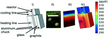 | ||
| Fig. 6 (i) Labelled reactor setup (ii) microreactor (iii) simulated temperature profile of microreactor (iv) simulated temperature profile of reactor with aluminium enclosure. | ||
Method applicability
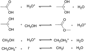
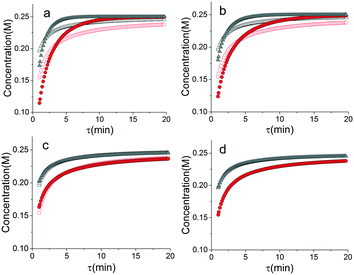
For many applications, more complex reactions and mechanisms are of greater interest. The usefulness of the proposed method is its scale independence, i.e., accurate representation of slow and fast reactions. The caveat being that more specialized experimental setups will be required for cases that are more complex. As an example, we simulated an esterification reaction and determined what conditions will be required to accurately determine the correct parameters in three different scenarios. The reaction follows a two-step mechanism with a two-step side reaction with methanol (Scheme 2).43 The parameter values chosen to simulate an actual experiment were adjusted between different scenarios in order to consider what happens for reactions with relative fast, slow and normal reaction rates.For the base case, the ‘normal’ reaction rate, we applied the procedure described earlier, namely fitting results of simultaneous residence time ramps and temperature ramps up and down (Fig. 7a). The same ramp conditions were then used to fit data for a fast reaction with very good agreement in the results (Fig. 7b). When we attempted those same conditions with a slow version of this reaction, we could not capture trends in the data (Fig. 7c.i). Decreasing the residence time ramp rate did not yield better results (Fig. 7c.ii). In order to fit the data, we needed to both decrease the residence time ramp rate as well as the temperature ramp rate. This example demonstrates that the ramp approach can be tuned to different reaction rates. The ramp rates had to be changed in order that the variables being ramped (temperature, residence time) can cover the measured variable (concentration) changes sufficiently.
Correct mechanism assumption
Another important topic in reaction kinetics analysis is whether or not the proper mechanism is assumed. Just as the two temperature ramps were sufficient to calculate the correct parameters in the cases earlier, it is also possible to use the simultaneous ramp data to discriminate between mechanisms given that the experiments sufficiently span the reaction space. We chose to demonstrate this ability with a simple example of a one-step reaction where the rate had a first order dependence on one reagent and a second order dependence of the other reagent. In this example, the product was monitored. Again, we simulated the simultaneous temperature and residence time ramps, but assumed a 3% normally distributed error in the measured results. Of the four potential models, we found two mechanisms that fit the data quite well with the correct one fitting the data most accurately (Table 1). In Fig. 8, the four potential models are compared with the actual model. This qualitatively shows that the two ramp experiments were able to, in this simple case, distinguish between the two models.| Model | log(A) | E/R/1000 | R 2 |
|---|---|---|---|
| kC A C B 2 | 5 | 2 | — |
| k I C A C B | 1.38 | 1.63 | 0.739 |
| k II C A 2 C B | 2.91 | 1.80 | 0.814 |
| k III C A 2 C B 2 | 6.83 | 2.22 | 0.987 |
| k IV C A C B 2 | 5.16 | 2.05 | 0.999 |
Conclusions
This work demonstrates a promising approach to quickly collecting accurate kinetic data in continuous flow. By utilizing microreactors with dynamic flow and temperature experiments, we were able to quickly generate robust kinetic data in a fraction of the time it would have taken for traditional approaches. This method is proposed as a general platform that allows for the tuning of experimental parameters for various reaction rates. The approach stands on its own but choice experimental setup is important to its accuracy. In the cases reported, only residence time and temperature were ramped. Nevertheless, the method could be scaled to handle more complex mechanisms where not only residence times and temperature but equivalents and initial concentrations are varied as well.Nomenclature
| V r | Reactor volume (μL) |
| V d | Dead volume between reactor exit and measurement (μL) |
| T | Reactor temperature (°C) |
| t | Time (min) |
| t i | Time when fluid element enters reactor |
| t f | Time when fluid element exits reactor |
| τ | Residence time in reactor (min) |
| τ ins | Instantaneous residence time ramps |
| Q total | Total flowrate into the reactor (μL min−1) |
| t m | Time measurement is taken (min) |
| θ | Scaled reaction parameters |
| θ up | Reaction parameters from T ramp up experiment |
| θ down | Reaction parameters from T ramp down experiment |
| θ u+d | Reaction parameters from T ramp up and down experiment |
| θ const-T | Reaction parameters from constant T experiments |
| Ĉ | Simulated concentration (M) |
| C | Measured concentration (M) |
| α | Slope of τ vs. t ramp |
| Pe | Peclet Number |
| U | Average velocity in reactor (m min−1) |
| L | Reactor length (m) |
Conflicts of interest
There are no conflicts to declare.Acknowledgements
This work was supported by Novartis.Notes and references
- J. W. Moore and R. G. Pearson, Kinetics and Mechanism, Wiley, Hoboken, 1981 Search PubMed.
- T. P. Labuza, J. Chem. Educ., 1984, 61, 348–358 CrossRef CAS.
- C. W. Coley, R. Barzilay, T. S. Jaakola, W. H. Green and K. F. Jensen, ACS Cent. Sci., 2017, 3, 434–443 CrossRef CAS PubMed.
- M. H. S. Segler and M. P. Waller, Chem. – Eur. J., 2017, 23, 5966–5971 CrossRef CAS PubMed.
- M. A. Kayala and P. Baldi, J. Chem. Inf. Model., 2012, 52, 2526–2540 CrossRef CAS PubMed.
- G. Jas and A. Kirschning, Chem. – Eur. J., 2003, 9, 5708–5723 CrossRef CAS PubMed.
- P. Watts and J. Haswell, Chem. Soc. Rev., 2005, 34, 235–246 RSC.
- J. P. McMullen and K. F. Jensen, Annu. Rev. Anal. Chem., 2010, 3, 19–42 CrossRef CAS PubMed.
- K. F. Jensen, B. J. Reizman and S. G. Newman, Lab Chip, 2014, 14, 3206–3212 RSC.
- S. V. Ley, D. E. Fitzpatrick, R. J. Ingham and R. M. Meyers, Angew. Chem., Int. Ed., 2015, 54, 3449–3464 CrossRef CAS PubMed.
- M. B. Plutschack, B. Pieber, K. Gilmore and P. H. Seeberger, Chem. Rev., 2017, 117, 11796–11893 CrossRef CAS PubMed.
- R. J. Ingham, C. Battilocchio, D. E. Fitzpatrick, E. Sliwinski, J. M. Hawkins and S. V. Ley, Angew. Chem., 2015, 127, 146–150 CrossRef.
- D. Ghislieri, K. Gilmore and P. H. Seeberger, Angew. Chem., Int. Ed., 2015, 54, 678–682 CAS.
- A. Adamo, R. L. Beingessner, M. Behnam, J. Chen, T. F. Jamison, K. F. Jensen, J. M. Monbaliu, A. S. Myerson, E. M. Revalor, D. R. Snead, T. Stelzer, N. Weeranoppanant, S. Y. Wong and P. Zhang, Science, 2016, 352, 61–67 CrossRef CAS PubMed.
- L. Malet-Sanz and F. Susanne, J. Med. Chem., 2012, 55, 4062–4098 CrossRef CAS PubMed.
- C. J. Mallia and I. R. Baxendale, Org. Process Res. Dev., 2016, 20, 327–360 CrossRef CAS.
- L. Kupracz and A. Kirschning, Adv. Synth. Catal., 2013, 355, 3375–3380 CrossRef CAS.
- S. Newton, S. V. Ley, E. C. Arce and D. M. Grainger, Adv. Synth. Catal., 2012, 354, 1805–1812 CrossRef CAS.
- F. J. Strauss, D. Cantillo, J. Guerra and C. O. Kappe, React. Chem. Eng., 2016, 1, 472–476 CAS.
- D. Cambie, C. Bottecchia, N. J. W. Straathof, V. Hessel and T. Voel, Chem. Rev., 2016, 116, 10276–10341 CrossRef CAS PubMed.
- M. Baumann and I. R. Baxendale, React. Chem. Eng., 2016, 1, 147–150 CAS.
- T. Fukuyama, Y. Fujita, M. A. Rashid and I. Ryu, Org. Lett., 2016, 18, 5444–5446 CrossRef CAS PubMed.
- N. J. W. Straathof, S. E. Cramer, V. Hessel and T. Noel, Angew. Chem., Int. Ed., 2016, 55, 15549–15553 CrossRef CAS PubMed.
- R. A. Green, D. Pletcher, S. G. Leach and R. C. D. Brown, Org. Lett., 2016, 18, 1198–1201 CrossRef CAS PubMed.
- Y. Matsumura, Y. Yamji, H. Tateno, T. Kashiwagi and M. Atobe, Chem. Lett., 2016, 45, 816–818 CrossRef CAS.
- B. J. Reizman and K. F. Jensen, Acc. Chem. Res., 2016, 49, 1786–1796 CrossRef CAS PubMed.
- V. Sans, L. Porwol, V. Dragone and L. Cronin, Chem. Sci., 2015, 6, 1258–1264 RSC.
- N. Holmes, G. R. Akien, R. J. D. Savage, C. Stanetty, I. R. Baxendale, A. J. Blacker, B. A. Taylor, R. L. Woodward, R. E. Meadows and R. A. Borne, React. Chem. Eng., 2016, 1, 96–100 CAS.
- H. Song and R. F. Ismagilov, J. Am. Chem. Soc., 2003, 125, 14613–14619 CrossRef CAS PubMed.
- P. J. Nieuwland, R. Segers, K. Koch, J. C. M. van Hest and F. P. J. T. Rutjes, Org. Process Res. Dev., 2011, 15, 783–787 CrossRef CAS.
- J. P. McMullen and K. F. Jensen, Org. Process Res. Dev., 2011, 15, 398–407 CrossRef CAS.
- B. J. Reizman and K. F. Jensen, Org. Process Res. Dev., 2012, 16, 1770–1782 CrossRef CAS.
- S. Mozharov, A. Nordon, D. Littlejohn, C. Wiles, P. Watts, P. Dallin and J. M. Girkin, J. Am. Chem. Soc., 2011, 133, 3601–3608 CrossRef CAS PubMed.
- J. S. Moore and K. F. Jensen, Angew. Chem., Int. Ed., 2014, 53, 470–473 CrossRef CAS PubMed.
- S. Schwolow, F. Braun, M. Rädle, N. Kockmann and T. Röder, Org. Process Res. Dev., 2015, 19, 1286–1292 CrossRef CAS.
- C. A. Hone, N. Holmes, G. R. Akien, R. A. Bourne and F. L. Muller, React. Chem. Eng., 2017, 2, 103–108 CAS.
- J. S. Moore, C. D. Smith and K. F. Jensen, React. Chem. Eng., 2016, 1, 272 CAS.
- D. G. Blackmond, Angew. Chem., Int. Ed., 2005, 44, 4302–4320 CrossRef CAS PubMed.
- G. Taylor, Proc. R. Soc. London, Ser. A, 1953, 219, 186–203 CrossRef CAS.
- K. D. Nagy, B. Shen, T. F. Jamison and K. F. Jensen, Org. Process Res. Dev., 2012, 16, 976–981 CrossRef CAS.
- V. Amarnath, D. C. Anthony, K. Amarnath, W. M. Valentine, L. A. Wetterau and D. G. Graham, J. Org. Chem., 1991, 56, 6924–6931 CrossRef CAS.
- M. W. Bedore, N. Zaborenko, K. F. Jensen and T. F. Jamison, Org. Process Res. Dev., 2010, 14, 432–440 CrossRef CAS.
- R. Ronnback, T. Salmi, A. Vuori, H. Haario, J. Lehtonen, A. Sundqvist and E. Tirronen, Chem. Eng. Sci., 1997, 52, 3369–3381 CrossRef CAS.
| This journal is © The Royal Society of Chemistry 2018 |

