 Open Access Article
Creative Commons Attribution 3.0 Unported Licence
Statistics of the network of organic chemistry†
Philipp-Maximilian
Jacob
and
Alexei
Lapkin
 *
*
Department of Chemical Engineering and Biotechnology, University of Cambridge, Cambridge, UK. E-mail: aal35@cam.ac.uk
First published on 19th January 2018
Abstract
Organic chemistry can be represented as a network of reactions and studied by mathematical tools of graph theory. In this paper, the structure of a network of organic reactions has been studied using several graph theory metrics. The network was based on a section of chemical space downloaded from Reaxys. The studied area of chemistry corresponds to the chemistry of terpenes and includes 12![[thin space (1/6-em)]](https://www.rsc.org/images/entities/char_2009.gif) 238
238![[thin space (1/6-em)]](https://www.rsc.org/images/entities/char_2009.gif) 931 species and 12
931 species and 12![[thin space (1/6-em)]](https://www.rsc.org/images/entities/char_2009.gif) 939
939![[thin space (1/6-em)]](https://www.rsc.org/images/entities/char_2009.gif) 422 reactions after filtering of an initial set of 35 million reactions. The analysis of the network statistics confirmed that the network was scale-free, as was reported in the earlier literature from the analysis of a much smaller network. Many networks in other technological or non-technological areas show that nodes have a preference as to whether they connect to highly connected or scarcely connected nodes, but for chemistry no such trend was observed. It was found that the network of reactions exhibits “small world” behaviour and in simile to the ‘six degrees of separation’ encountered in social networks, on average, any molecule could be made from any other molecule in six synthesis steps. Scale-free networks have hubs in their wiring pattern. By investigating whether these hubs are not only well studied but also frequently used, it was found that they concentrated a large share of the network's load onto themselves, showing that the network's structure impacts the usage of chemistry, or vice versa, implying a hierarchy of molecules.
422 reactions after filtering of an initial set of 35 million reactions. The analysis of the network statistics confirmed that the network was scale-free, as was reported in the earlier literature from the analysis of a much smaller network. Many networks in other technological or non-technological areas show that nodes have a preference as to whether they connect to highly connected or scarcely connected nodes, but for chemistry no such trend was observed. It was found that the network of reactions exhibits “small world” behaviour and in simile to the ‘six degrees of separation’ encountered in social networks, on average, any molecule could be made from any other molecule in six synthesis steps. Scale-free networks have hubs in their wiring pattern. By investigating whether these hubs are not only well studied but also frequently used, it was found that they concentrated a large share of the network's load onto themselves, showing that the network's structure impacts the usage of chemistry, or vice versa, implying a hierarchy of molecules.
1. Introduction
With the growth of online reaction databases, an increasing amount of reaction data are available to assist in the design of synthetic routes: Reaxys alone contains in excess of 40 million reactions.1,2 The way how we currently use databases is to search for individual transformations, or for possible multi-step syntheses using a stepwise search through the available database interfaces, such as SciFinder, Reaxys, Wiley ChemPlanner,3 ChemSpider or SPRESI. However, it has recently been shown that using the data as a whole by means of network traversal algorithms allows a researcher to ask more questions of the data.4–11 Thus, one can look at optimisation of a range of feedstocks used by a company,6 optimising parallel synthesis routes,10 identifying one-pot conversions,8 monitoring the use of controlled substances more effectively,7 or investigating reactivity trends of functional groups.9 In our own work, we have shown the use of large chemical datasets to develop reaction sequences by running a targeted network search, taking molecular structural information into account; the reaction sequences are then evaluated in terms of a range of performance metrics.12,13In addition to synthesis planning, an alternative potential use of chemical data networks is the discovery of new reactions. This is an inverse problem: instead of asking a chemical question from the network, we intend to ask a mathematical question, with a hypothesis that the structure of the chemical network contains implicit chemical information, which we may reveal in the form of yet unknown transformations. In order to proceed with such an investigation, we think that it is important to understand the structure of the data better. It ought to be noted that the use of graph theory in the case of reaction networks is different from, and should not be confused with, the retrosynthesis approach of Corey and Wipke, where molecules were represented as graphs.14
The algorithmic uses of chemical data published to date exploit the fact that chemical data can be represented by a network and traversed as a graph. This was first discussed in ref. 4–6 using a dataset of 9![[thin space (1/6-em)]](https://www.rsc.org/images/entities/char_2009.gif) 293
293![[thin space (1/6-em)]](https://www.rsc.org/images/entities/char_2009.gif) 250 reactions from what was then the Beilstein database. The dataset used in these early studies was fairly small, compared to the size of, for example, the Reaxys database today.1,4 It is, therefore, useful to examine the larger dataset available today and to expand the analysis to the metrics of graphs not used in the earlier analyses of the chemistry data, as this may reveal further general trends in the development of organic synthesis.
250 reactions from what was then the Beilstein database. The dataset used in these early studies was fairly small, compared to the size of, for example, the Reaxys database today.1,4 It is, therefore, useful to examine the larger dataset available today and to expand the analysis to the metrics of graphs not used in the earlier analyses of the chemistry data, as this may reveal further general trends in the development of organic synthesis.
This paper will repeat some of the analyses carried out earlier,4–6 but on a larger data set, and will investigate a number of additional graph theoretical metrics to quantify and study the network's dynamics. Though the metrics employed have differing levels of granularity, they are all statistical in nature and, thus, provide averages. Investigation of these metrics is a necessary step to allow the application of either more sophisticated graph theoretical concepts or an in-depth study of a certain area of chemistry using the network, but in themselves cannot be expected to yield information about a specific reaction or class of reactions.
More specifically, this paper will aim to answer the question what statistical properties can be observed for the section of the network studied here. It will seek to reassess if the network is indeed scale-free, whether it exhibits ‘small-world’ behaviour, and if it displays evidence of a hierarchy of nodes. This will be accomplished by investigating the degree distribution of the network, its assortativity, the existence of degree correlations and the shortest path lengths observed. Furthermore, the clustering coefficient and betweenness centrality will be investigated. Taking the results from these analyses, it will be possible to form a more complete picture of the network. Ultimately, this can be used to gain a better understanding of the chemical knowledge contained within the network. We deliberately do not focus on the historical development of the network, for example, the development of network ‘hubs’, as we are aware of a separate focused study on this sole topic to be completed shortly.
Given that graph theoretical tools do not form part of the standard chemistry or chemical engineering toolset, each of the investigated metrics is introduced in detail and its theoretical background is given in the following section. The methods used to quantify the statistics are described in the Methodology section and an interpretation of their relevance to our understanding of chemistry is given in detail in the Results and discussion section. However, a brief outline of their significance is as follows: scale-free networks follow precisely defined evolution patterns allowing conclusions about further development of the chemical landscape to be made, while also implying the existence of ‘hubs’, meaning that the average distance between two molecules is greatly reduced. The assortativity and the degree correlation, collectively, measure the mixing patterns of the network. This means that it reveals information whether a given molecule, on average, is more likely to connect to a hub or a molecule in the periphery; in other words, it might reveal whether a platform molecule is likely to react into a specialised molecule or another platform molecule. Studying the small-world behaviour of the network is very important in understanding how long the paths between two molecules are on average, i.e. how many reactions it takes to synthesise one out of the other, thus giving insights into how the network can be navigated more optimally. Analysing the betweenness centrality finally allows an assessment of the importance of molecules to synthesis routes in general by quantifying what share of paths runs via them.
2. Theory
2.1. Introduction to graph theory
The foundation of the field of graph theory is often associated with Leonhard Euler who “discovered” it in 1736.15,16 From initially being a purely mathematical topic, it has subsequently spread into fields as wide as the internet, sociology, biology, chemistry, physics, neuroscience and even history and English literature.15,17–20 The terms “graph” and “network” are often used interchangeably, although there is a subtle difference between them. A graph is primarily an abstract mathematical object that does not necessarily consider its realisation in nature. A network, on the other hand, is a “real-life” object as opposed to a purely mathematical one.21The first formal model generating a graph was that of a random graph, also referred to as the Erdős–Rényi model.22 In it, N nodes (the terms node and vertex are used interchangeably in the literature) are added to a network and then edges are added between two nodes according to a probability p.23 This means that the node degrees, i.e. the number of connections a given node has, follow a Poisson distribution17 roughly centred around an average degree, ![[k with combining macron]](https://www.rsc.org/images/entities/i_char_006b_0304.gif) .23
.23
With the rise in computing power, it became clear that most networks do not follow the trends of a random graph. Instead, many networks deviate by showing “small world” behaviour, a degree distribution that follows a power-law rather than a Poisson distribution, high degrees of clustering, and degree correlations between connected vertices.17,23,24 These clear, non-random deviations in topology required the field of graph theory to develop new models to describe the organising principles of real networks.17,18,25
A large number of real networks exhibit a power-law degree distribution, in stark contrast to the Poisson distribution predicted by the Erdős–Rényi model.25 This was first discovered by de Solla Price in 1965.26 It was independently rediscovered in 1999 (ref. 27) and subsequently achieved prominence as the Barabasi–Albert model, describing what was termed a ‘scale-free network’.17,18,28 Though this name may appear counter-intuitive, it acknowledges the fact that while a random network has a characteristic scale in the average degree, around which its degree distribution is centred, the scale-free network has no such single scale. An important caveat is that though the overall network may have no scale in its degree distribution, both the other properties of the network and the degree distribution of sub-networks may have scales present.18,29
The power-law degree distribution means that many nodes have very few connections, while a few nodes have a very large number of connections. This means that a scale-free network exhibits hubs, which are vertices that are linked to a significant fraction of the total number of edges in the network,17 affecting the properties of the network. For example, this means that the average distance between nodes, i.e. the number of edges that need to be traversed en route between the two, is lower than that in a random network,30 or that the network exhibits a much greater degree of clustering than might be expected of a comparable random network.31
A number of recent studies have shown the existence of a hierarchical structure in many real-life networks,32–34 in which groups of vertices can be subdivided into smaller clusters of vertices, which each divide into yet smaller groups over several iterations.23,35,36 This phenomenon was first observed when examining metabolic networks.37 These networks on the one hand exhibited very high degrees of clustering, indicative of a modular architecture, while on the other hand having a power-law degree distribution. This was surprising as a highly modular architecture greatly restricts the degree distribution, while a scale-free architecture runs counter to a modular organisation. This apparent contradiction was overcome by using a heuristic model that combined nodes into densely connected local clusters, which in turn combined into less dense, larger groups, which again combined into even less cohesive larger groups, thus allowing communication between the densely clustered modules via a small number of hubs.23,32 As a consequence, a hierarchical network is able to explain local clustering and modularity, short path lengths, and scale-free degree distributions.23,32,38
Clustering can be quantified with the clustering coefficient, which measures the amount of interlinking between neighbours of a given node. It has been argued that a key signature of a hierarchical network is the existence of an inverse scaling between the clustering coefficient and the degree. This is caused by the fact that increasing the cluster size, which means an increase in the degree, leads to a decreasing degree of interlinking, meaning a decreasing clustering coefficient. This gives rise to a power-law behaviour. Evidence of this was reported in a number of sources,23,32,37,39–42 though Soffer and Vázquez contest this claim, arguing that the trend observed is merely a consequence of correlations between the degrees of neighbouring nodes.24
In practice, real-life networks do not necessarily exactly fit into one of the presented categories and are thus classified as “complex networks”.43 Despite spanning a vast field of disparate topics, it has been found that many of these networks are characterised by the same topological properties.30 One such property, for example, is the “small world effect”, first popularised in sociology. It describes the fact that most nodes can be connected via only a few edges,44 far fewer than expected by chance. This was found to be the case in virtually all computational or biological networks.15,23 Similarly, a very common phenomenon in complex networks is a degree correlation, where it is possible to establish a correlation between a vertex's degree and the degree of the vertices it connects to, i.e. a correlation between the number of connections of a node and the number of connections of its neighbours.30,44,45
Another interesting question is estimating the importance of a given vertex to the network. This is possible by finding the shortest route connecting all possible combinations of vertices in the network and then measuring the fraction of these routes running via this vertex. The result of this is referred to as ‘betweenness centrality’.30 The metrics used to study the network of organic chemistry in this paper are introduced in detail below.
2.2. Degree distribution
One of the fundamental properties of a network is the so-called “degree”. The degree of node i, ki, gives the number of edges connected to a given node. In the case of a directed network, such as is the case here, each edge has a “source” and a “target” with the directionality representing, in this case, the direction in which a reaction proceeds. This means that it is not merely sufficient to count the number of edges connected to a node, but that the measure needs to be further refined into an “out-degree”, kout, giving the number of edges emanating from the node, and an “in-degree”, kin, giving the number of edges which have the node as the target.According to ref. 4 and 6, the Network of Organic Chemistry exhibits scale-free behaviour and thus its degree distribution follows a power law, where the probability, P(k), of observing a given degree, k, is given by eqn (1) for both the in-degree, kin, and the out-degree, kout.
| P(k) ∝ k−γ | (1) |
According to the literature,4,6 the respective power-law exponents, γin and γout, take the approximate values of 2.7 and 2.1, respectively. The network will therefore be analysed to see if the same behaviour can be observed to verify its scale-free nature.
For uncorrelated networks, the degree distribution completely describes the statistical properties of the network. For most real networks, however, there is a correlation between the degrees of neighbouring nodes,30 which shall be further analysed in the following section.
2.3. Assortativity
In any given network, one would expect to find a difference in vertex properties between neighbouring vertices. This is of particular interest in sociology, where a question of interest might be whether people with many social connections largely connect with other people with many connections or with people with few connections. In epidemiology, the study of this variation could be very useful in giving insights into how quickly an epidemic might spread or how effective a vaccination campaign might be, whilst in technology networks, such as the internet, it could lend insights into the resilience of the network against random node failure, by servers going off-line, or against directed node failure, through targeted hacking attacks or computer viruses.Linking of nodes of similar properties to nodes with similar properties occurs in networks exhibiting assortative mixing (as shown in Fig. 1).46 In sociology, this might be the case of gregarious people connecting largely to other gregarious people. The case of nodes with a given magnitude for a given vertex property preferentially linking to nodes with a different magnitude for the same vertex property is called disassortative mixing (as illustrated in Fig. 2).46 This can be observed, for example, in the internet, where the backbone structure of the internet means that nodes of high degree counts link to nodes of low degree counts.
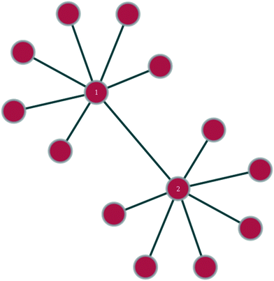 | ||
| Fig. 1 Within the shown section of a network, nodes 1 and 2 exhibit assortative mixing in that two nodes of similar degree connect to each other. | ||
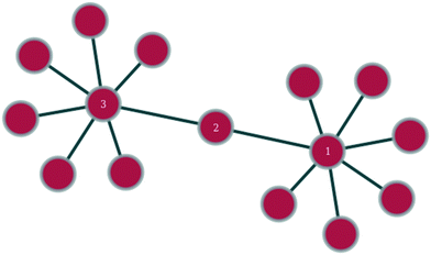 | ||
| Fig. 2 Within this section of a network, nodes 1 and 3 exhibit disassortative mixing in that two nodes of similar degree preferentially connect to a node of a different degree count. | ||
In order to quantify this effect, Newman proposed an assortativity coefficient, r, which quantifies whether the network exhibits assortative, no, or disassortative mixing.47 In the case of a directed network, r takes the form of eqn (2),47
 | (2) |
Finally, qk and qj can be found as follows:
 | (3) |
As a consequence, we find that 0 < r ≤ 1 for all networks with assortative mixing, zero in the absence of a mixing structure, and −1 ≤ r < 0 in the case of disassortative mixing.47
The definition is complicated by the fact that it has to deal with directed networks. In the undirected case, the definition is intuitive in that it considers only a single quantity, the degree. The reader is referred to ref. 47 for the form of the undirected assortativity coefficient. When expanding it to directed networks, the above given definition now measures similarity in terms of two different quantities for a given node pair, in-degree and out-degree. To alleviate this contradiction, Piraveenan et al. proposed an out- and an in-assortativity, rout and rin, respectively, which now measure the propensity to link to a node by considering only a single property.48 This form shall be used in the further analysis:
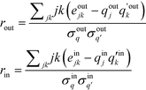 | (4) |
 is the probability distribution of an edge going into a node of out-degree k. Furthermore, σoutq is the standard deviation of qoutj and σoutq′ is that of
  . Similar definitions apply to rin.
It appears to be the case that social networks are largely assortative while biological and technological networks exhibit disassortative mixing.17,23,47 The reason for the internet displaying disassortative mixing is that the high-degree vertices are connectivity providers, or directories, which by definition tend to connect to the “little people”.47 However, the observed disassortative behaviour may be an artefact of the sampling carried out.47
Other authors caution that the often observed assortative trend may simply be an artefact caused by the fact that many of the studied cases were, in fact, implicit projections of bipartite networks. This illustrates the danger of placing too much importance on generalisations about the assortativity or disassortativity structures of given classes of networks, or not considering how the studied data has actually been collected and presented.49
If the constraint that no two vertices may be connected by more than one edge is imposed, then high-degree vertices seemingly repel one another, leading to disassortative mixing. In the case of the internet, for example, crawlers often record websites linking to another website multiple times only once. As a consequence, the observed behaviour, at least in parts, may be an artefact of the chosen representation as opposed to the underlying properties of the network.47,50
2.4. Degree correlation
As can be observed from the previous section, the assortativity of a network is closely related to the correlation of degrees between connected vertices, ejk. This correlation can be further analysed by studying the nearest neighbour average connectivity,![[k with combining macron]](https://www.rsc.org/images/entities/i_char_006b_0304.gif) nn, which is related to the degree correlation as follows, but is in practice easier to calculate than the degree correlation:17,51,52
nn, which is related to the degree correlation as follows, but is in practice easier to calculate than the degree correlation:17,51,52 | (5) |
2.5. Average shortest path length
The average shortest path length, or average shortest path distance, is a metric useful in assessing a network's topology. This is defined as follows:53,54
 | (6) |
In 1967, Milgram described a phenomenon termed “small world network”.55,56 It was first used in the context of “six degrees of separation”, the idea that any person could pass a message to any other person via, on average, six other people. Though the parallel to social networks might be striking, the small world network phenomenon is by no means restricted to an average shortest path length of six. More rigorously defined, a network is considered to exhibit small world effects if the average shortest path length scales with the logarithm of the number of vertices, i.e. ∝ log
∝ log![[thin space (1/6-em)]](https://www.rsc.org/images/entities/char_2009.gif) N or slower.18,23,52,57
N or slower.18,23,52,57
2.6. Clustering coefficient
A related concept to that of whether well-connected people are more likely to form friendships with other well-connected people or not is the question whether the friend of your friend is also your friend. By expressing this in graph theoretical terms, it is often found in real networks that if vertex A is connected to vertex B and vertex B to vertex C, then there is a heightened probability of vertex A also connecting to vertex C.18 In order to express this mathematically, it is possible to study whether the number of triangles in a network is greater than expected by measuring the mean probability that two vertices that are neighbours of the same other vertex are neighbours themselves.58 This is measured by the global clustering coefficient, C, as follows:18 | (7) |
A useful modification of the clustering coefficient is the local clustering coefficient calculated for each vertex i, ci, as proposed by Watts and Strogatz.18,59 In the case of an undirected network, it is defined as the fraction of the number of edges, ni, amongst the nearest neighbours of the given vertex i and the maximum possible number of edges should all of node i's neighbours be connected to each other,  :23,37,52,59
 | (8) |
In this case, the network is directed, meaning that the direction of the edges needs to be considered too, changing the overall expression. The literature on the topic, however, cannot agree on the equation for a directed network (ref. 43 and 60 use conflicting versions). The literature precedent of ref. 32 and 52 is followed in this study, and the network is treated as undirected.
While the shortest path length gives a measure of the number of friends in a typical chain of connections linking two people, the clustering coefficient, continuing the simile of social networks, can be described more intuitively as a measure of how much the friends of user i are also friends with each other, and thus provides an estimate of the “cliquishness” of a friendship circle.59
Though this undoubtedly is a figure describing the network topography, it is merely an average. A more interesting question is how the clustering coefficient varies with a node's degree.30,52
Re-examining eqn (8), it becomes apparent that for a degree of 1, c needs to be defined as 0. Having done so, it is possible to define the degree-dependent average clustering coefficient, ![[c with combining macron]](https://www.rsc.org/images/entities/i_char_0063_0304.gif) (k):52,61
(k):52,61
 | (9) |
In eqn (9), nk denotes the number of nodes of degree k, while the summation term is the sum of the clustering coefficients across all N nodes in the network; δki, k is the Kronecker delta and ki is the degree of node i. The degree-dependent average clustering coefficient in turn is related to the average clustering coefficient, ![[c with combining macron]](https://www.rsc.org/images/entities/i_char_0063_0304.gif) , as follows:62
, as follows:62
 | (10) |
2.7. Betweenness centrality
The betweenness of a given vertex i, bi, is the number of shortest paths between all pairs of vertices in the network that go through this vertex. If there are multiple paths between a given pair, then the paths that do pass through the vertex contribute fractionally.52If we accept the supposition that the shortest path is an indicator of the ideal route between two vertices, then the betweenness of a given vertex is a measure of the amount of traffic that it sees. Therefore, it is a measure of its centrality in the network leading to the term betweenness centrality.52 Similarly, it is possible to define an edge centrality.18,57 This concept has been discussed in intuitive terms since at least 1948.63 However, an algebraic definition was first published only in 1977 by Freeman,63 in the context of relaying information in a social network. If we take a pair of points, i, j, then the number of shortest paths connecting these points, so-called geodesics, shall be denoted by g(i, j). If we assume that all paths are equally likely to be the path along which the message is transmitted, then the probability of a given path being used is  . If we consider a point k, then the likelihood that this point is along the path “chosen” by the message is the number of geodesics between i and j on which k lies, with gk (i, j) multiplied by the likelihood of any of these paths being the “chosen” path.63 This value shall be called partial betweenness of k, bk (i, j):
 | (11) |
To determine the betweenness centrality of a point, k, with regards to the entire network, we need to sum all the partial betweennesses for all pairs of vertices where i ≠ j ≠ k:63,64
 | (12) |
Calculating the betweenness centrality requires knowledge of the shortest paths in the network. If this is unknown, a search algorithm must instead be used. The betweenness of a vertex or edge can also be expressed in terms of the likelihood of it being visited by the used search algorithm.17
This measure is obviously sensitive to the number of nodes in a network and the number of connections involving k. Particularly the former can have an undesirable impact on the meaning of the magnitude of the betweenness when comparing the value across networks. Freeman illustrates this with a short example: if we take a node i, in a network of five nodes, with a betweenness value of bi = 6, and a node j in a network of 25 nodes, also with a betweenness value of bj = 6, then both points have the same importance in absolute terms, when it comes to their ability to control communications. Their relative potential, however, is very different. While i is involved in more than half of the communications, j is only involved in slightly more than 1%.63 It may therefore be desirable to normalise bk by the number of pairs of vertices in the network, not including k,  :63
:63
 | (13) |
Another property of potential interest is the central point dominance. It gives a measure of a network's centrality to the extent that a single point can control its communications. It is defined as the difference in the normalised centrality of a given point k,  , and the normalised centrality of the vertex v*, which is the vertex with the largest normalised betweenness centrality, summed across all vertices, divided by the number of vertices minus one:63
 | (14) |
The central point dominance is, in other words, the average difference in centrality between the most central point and all others, taking a value of 1 for a wheel or star, and 0 for a completely decentralised network where the centralities of all nodes are equal.63
As mentioned previously, the internet is a major example of a network whose suspected scale-free behaviour has been extensively studied in the literature. The internet is composed of central “backbones”, for example transatlantic cables, connecting different regions, for example countries, that in turn connect smaller subsections of the network, for example regions within a country. As a consequence, one would expect that the backbones would carry a greater load as a proportionally greater number of connections in the internet might be expected to run via these. Or, if analysing the internet in terms of nodes rather than edges, one might expect that the “entrance” and “exit” nodes carry a greater load. Though it can be difficult to measure the load in a network, one might expect that this variation of load, and the resulting hierarchy of connections, might manifest itself in the structure of the network itself. The question of interest here is whether the hub molecules that have already been identified in the degree analysis do indeed also carry a greater share of the load of the network, which would provide quantitative evidence for the existence of a hierarchy of nodes.
As outlined earlier, the number of geodesics running through a given node, as measured by the betweenness centrality, can serve as a proxy measure for the load of a given node in a network. In order to investigate a potential hierarchical organisation, the average degree-dependent betweenness is of greater interest. Mathematically, this quantity is defined as follows:52
 | (15) |
3. Methodology
3.1. Degree distribution
A network of reactions was constructed based on the reactions contained in Reaxys.2 All reactions involving limonene as the reactant were downloaded. The choice of the starting point in the data search was dictated by the specific problem statement within a project on developing potential transformations of terpene sources as a waste bio-feedstock into useful chemicals.12 All product species from these reactions were individually queried to obtain all reactions starting from each of these species. This was repeated to obtain data containing four reaction steps to obtain a network of adequate size. This was written to a file and incomplete reactions were deleted. The data mapped the network explicitly, depicting all contained products. Information about the reactants, however, existed only implicitly in so far as that they featured as information in the reactions retrieved for the products, but there was no guarantee that this was a complete set. To overcome this issue an additional search was run and all species that had been searched for as products were now searched for as reactants too. Thus, it was ensured that a complete and accurate picture of the reactions contained in Reaxys for the species searched for had been obtained.This process retrieved 50![[thin space (1/6-em)]](https://www.rsc.org/images/entities/char_2009.gif) 296
296![[thin space (1/6-em)]](https://www.rsc.org/images/entities/char_2009.gif) 475 reactions. After removing the duplicate entries in that list, 34
475 reactions. After removing the duplicate entries in that list, 34![[thin space (1/6-em)]](https://www.rsc.org/images/entities/char_2009.gif) 260
260![[thin space (1/6-em)]](https://www.rsc.org/images/entities/char_2009.gif) 049 reactions remained. This equates to close to 80% of reactions in Reaxys at the time.65 In its early phases, Reaxys sometimes aggregated reactions comprising several steps, created a new, duplicate entry for these and then marked these as multistep reactions to improve manual searchability. For this reason, inclusion of the multistep reactions skews the network's statistics and, thus, they were excluded from the analysis set. This brought the number of reactions down to 13
049 reactions remained. This equates to close to 80% of reactions in Reaxys at the time.65 In its early phases, Reaxys sometimes aggregated reactions comprising several steps, created a new, duplicate entry for these and then marked these as multistep reactions to improve manual searchability. For this reason, inclusion of the multistep reactions skews the network's statistics and, thus, they were excluded from the analysis set. This brought the number of reactions down to 13![[thin space (1/6-em)]](https://www.rsc.org/images/entities/char_2009.gif) 770
770![[thin space (1/6-em)]](https://www.rsc.org/images/entities/char_2009.gif) 205. Deletion of incomplete reactions, namely those that had either no products or no reactants declared in Reaxys, left the total number of reactions analysed at 12
205. Deletion of incomplete reactions, namely those that had either no products or no reactants declared in Reaxys, left the total number of reactions analysed at 12![[thin space (1/6-em)]](https://www.rsc.org/images/entities/char_2009.gif) 939
939![[thin space (1/6-em)]](https://www.rsc.org/images/entities/char_2009.gif) 422.
422.
The condensed and sanitised data set was converted into a network using Python scripts and an implementation of graph-tool in Python2.7.60 This was carried out by assigning each chemical species contained in the data set as a vertex in the network and then for each reaction connecting all reactants to all products via a directed edge going from the reactant to the product. Each node and edge was then annotated with various properties, such as Reaxys IDs, to allow their matching to a database entry. Multiple different wiring schemes are of course possible, ranging from the “all to all” scheme employed here on the one end of the spectrum to a “one to one” scheme, where only the heaviest reactant and product of each reaction are added to and linked in the network resulting in only one edge per reaction. Fialkowski et al. have carried out an investigation of the effects of the choice of the wiring scheme on the properties of the network and found them to be negligible.66
In order to analyse the degree distribution, the in-degree of every node in the network was then written to one file and the out-degree to another file. Firstly, given the fact that a power law is undefined for a value of k = 0, all nodes that had a degree of 0 were deleted from the respective file. Subsequently, the data were analysed using the Python package “powerlaw” in Python2.7.67
Seeing as the degree distribution is necessarily discrete, discrete=True was set in the code and estimate_discrete=False. Furthermore, it was specified that kmin = 1.0 as this represents the lowest possible degree a node can have under the power-law model. The “powerlaw” package was then used to fit the data to a power-law model. An important fact to bear in mind is that the probability density functions (pdf) of heavy-tailed distributions are notoriously noisy in their tail as the number of observations of a given value, in this case the degree, is very low in the tail. This makes it more convenient to use cumulative distribution functions (cdfs), expressing the likelihood of observing a value less than or equal to the given value.52,67,68 Using the cdf, it is possible to determine the slope, 1 − γ, and thus the degree exponent with far greater accuracy compared to using the degree distribution, while also showing possible truncation of the tail more clearly.69 The other approach towards smoothing out the fluctuation in the tail of the pdf is to use binning if employing bins of exponential length.69 Both techniques were employed here.
Perhaps more relevant is the question whether the data is best described using a power law. The log-likelihood ratio between two candidate models, R, was computed along with its significance value (p-value) using the “powerlaw” package.67 A positive value of the logarithm of the ratio of the likelihood of the first distribution and the likelihood of the second distribution indicates that the data is more likely to be described by the first distribution, in this case a power law, and a negative value indicates that the other candidate model provides a better explanation.67,68 Though R gives us an estimate of which distribution is more likely, it, like any other quantity, is subject to statistical fluctuations. Thus, if the true value of R is close to zero, a fluctuation can lead to a sign change, meaning that we cannot trust the value of R.68 For this reason, we also require the p-value as a measure of whether the observed sign of R is statistically significant. This means that if we observe a small value of p (ref. 68 suggests a cut-off of 0.1, in ref. 67 a cut-off of 0.05 was suggested), it is unlikely that the sign of R is the result of a chance fluctuation and, hence, is able to tell which model is favoured. If the p-value is large, the sign is most likely the result of a statistical fluctuation, and the test does not favour either model as a description of the observed data.
The defining feature of a power law is the fact that it displays a heavy-tailed distribution. For this reason, the goodness of fit using a power law is compared to that of a lognormal distribution and a stretched exponential distribution, which both exhibit heavy tails without following a power law.67 By definition, a heavy tail is not exponentially bounded. Thus, if the data is described more accurately by an exponential distribution, there is little argument for observing a heavy-tailed distribution, meaning that the data does not follow a power law.67 Finally, a truncated power law is tested for, representing a mixture of the exponential distribution and the power law.67
3.2. Assortativity
The assortativity was calculated for both the in- and the out-degree as well as the combined degree using a function implemented in graph-tool. This was done both when allowing parallel edges and when allowing only one edge so as to allow conclusions about the wiring scheme's impact on the value of the assortativity.3.3. Degree correlation
In practice, eqn (5) can be evaluated more easily by averaging the degree of all nearest neighbours of all nodes of degree k for all values of k, which can then be plotted against each other. If no correlation exists between the two degrees,![[k with combining macron]](https://www.rsc.org/images/entities/i_char_006b_0304.gif) nn (k) will be independent of k (i.e. r = 0),51,52,62 while an increasing function in k corresponds to assortative mixing and a decreasing function to disassortative mixing.42,44,62 For a perfectly assortative network, one would expect the points to fall onto the x–y diagonal. Naturally, this function can be calculated for the in-, out- and total-degree. The results of doing so will be shown subsequently.
nn (k) will be independent of k (i.e. r = 0),51,52,62 while an increasing function in k corresponds to assortative mixing and a decreasing function to disassortative mixing.42,44,62 For a perfectly assortative network, one would expect the points to fall onto the x–y diagonal. Naturally, this function can be calculated for the in-, out- and total-degree. The results of doing so will be shown subsequently.
3.4. Average shortest path length
The average shortest path length of the network under investigation was computed using the “distance_histogram” function in graph-tool,60 generating the number of shortest paths of a certain length existing in the network, which thus allows computation of . Similar to the degree distribution, it is possible to plot the probability distribution of obtaining a given shortest path length, P(
![[small script l]](https://www.rsc.org/images/entities/char_e146.gif) ), against the shortest path length,
), against the shortest path length, ![[small script l]](https://www.rsc.org/images/entities/i_char_e146.gif) , which was also carried out.
, which was also carried out.
In order to analyse the variation of  with the number of nodes in the network, all nodes were labelled with the date in which they first appeared in this network. Seeing as the publication dates of all the reactions in the network were retrieved from Reaxys, the earliest date of all edges incident and emanating from a given node was determined and used to label the given node. With this information, it was then possible to progressively add nodes and edges to the network by stepping forward in time and observing the change in
  . The network corresponding to the year 1900 contains 106
![[thin space (1/6-em)]](https://www.rsc.org/images/entities/char_2009.gif) 224 nodes gradually increasing to 12
224 nodes gradually increasing to 12![[thin space (1/6-em)]](https://www.rsc.org/images/entities/char_2009.gif) 238
238![[thin space (1/6-em)]](https://www.rsc.org/images/entities/char_2009.gif) 929 in the year 2016.
929 in the year 2016.
The distance histogram function allows computation of the histogram based on a pre-defined number of random samples of vertices drawn from the network, which was necessary in this case to reduce the overall computational time as, due to the very large size of the network, direct computation would be prohibitively expensive.
To analyse the variation in results with the number of nodes sampled, a number of trials were conducted, the results of which can be found in Table 1. In this case, a section of the NOC was used containing a total of 9![[thin space (1/6-em)]](https://www.rsc.org/images/entities/char_2009.gif) 012
012![[thin space (1/6-em)]](https://www.rsc.org/images/entities/char_2009.gif) 439 nodes.
439 nodes.
 and the required computation time for a given number of nodes sampled out of a sample network comprising a total of 9
![[thin space (1/6-em)]](https://www.rsc.org/images/entities/char_2009.gif) 012
012![[thin space (1/6-em)]](https://www.rsc.org/images/entities/char_2009.gif) 439 nodes. These values were computed using parallel processing on up to 24 cores.
439 nodes. These values were computed using parallel processing on up to 24 cores.  gives the deviation of the current value from the value when sampling all nodes in percent
| Number of samples | Fraction of sampled nodes [%] | [%] | Computation time [s] | |
|---|---|---|---|---|
10![[thin space (1/6-em)]](https://www.rsc.org/images/entities/char_2009.gif) 000 000 |
0.11 | 5.301 | 0.61 | 79 |
75![[thin space (1/6-em)]](https://www.rsc.org/images/entities/char_2009.gif) 000 000 |
0.83 | 5.227 | −0.80 | 550 |
100![[thin space (1/6-em)]](https://www.rsc.org/images/entities/char_2009.gif) 000 000 |
1.11 | 5.313 | 0.84 | 705 |
250![[thin space (1/6-em)]](https://www.rsc.org/images/entities/char_2009.gif) 000 000 |
2.77 | 5.273 | 0.08 | 1700 |
500![[thin space (1/6-em)]](https://www.rsc.org/images/entities/char_2009.gif) 000 000 |
5.55 | 5.277 | 0.15 | 3243 |
750![[thin space (1/6-em)]](https://www.rsc.org/images/entities/char_2009.gif) 000 000 |
8.32 | 5.277 | 0.15 | 5940 |
1![[thin space (1/6-em)]](https://www.rsc.org/images/entities/char_2009.gif) 000 000![[thin space (1/6-em)]](https://www.rsc.org/images/entities/char_2009.gif) 000 000 |
11.10 | 5.272 | 0.06 | 11![[thin space (1/6-em)]](https://www.rsc.org/images/entities/char_2009.gif) 297 297 |
3![[thin space (1/6-em)]](https://www.rsc.org/images/entities/char_2009.gif) 000 000![[thin space (1/6-em)]](https://www.rsc.org/images/entities/char_2009.gif) 000 000 |
33.29 | 5.274 | 0.09 | 26![[thin space (1/6-em)]](https://www.rsc.org/images/entities/char_2009.gif) 179 179 |
6![[thin space (1/6-em)]](https://www.rsc.org/images/entities/char_2009.gif) 000 000![[thin space (1/6-em)]](https://www.rsc.org/images/entities/char_2009.gif) 000 000 |
66.57 | 5.269 | 0.00 | 57![[thin space (1/6-em)]](https://www.rsc.org/images/entities/char_2009.gif) 565 565 |
9![[thin space (1/6-em)]](https://www.rsc.org/images/entities/char_2009.gif) 012 012![[thin space (1/6-em)]](https://www.rsc.org/images/entities/char_2009.gif) 439 439 |
100.00 | 5.269 | 0.00 | 87![[thin space (1/6-em)]](https://www.rsc.org/images/entities/char_2009.gif) 031 031 |
As can be seen very clearly from Table 1, the deviation from the actual value of  is minor even when sampling only 10
![[thin space (1/6-em)]](https://www.rsc.org/images/entities/char_2009.gif) 000 nodes, or 0.11% of the total network, with the deviation amounting to only 0.61%. When sampling roughly 3% of the nodes in the network, the error drops to around 0.10% while requiring a computational time of only 28 minutes.
000 nodes, or 0.11% of the total network, with the deviation amounting to only 0.61%. When sampling roughly 3% of the nodes in the network, the error drops to around 0.10% while requiring a computational time of only 28 minutes.
Consequently, it was decided to sample 3% of the nodes for the study of the variation of  with the number of nodes in the network providing a good trade-off between accuracy and speed.
In order to compute the average shortest path length for a number of given points in time, the network was sampled as described above and the average shortest path length was computed using eqn (6). This was repeated three times for each point in time, calculating the mean of the three values and the standard deviation. The standard deviation of these three points was used to give an idea of the spread of the measured samples.
3.5. Clustering coefficient
In order to analyse the clustering observed in the network, firstly, the global clustering coefficient was calculated using graph-tool. Next, in order to analyse the degree-dependent average clustering coefficient, the local clustering coefficient of each node was calculated in graph-tool. Having done so, a loop was written to cycle through all nodes in the graph. For each node, its total degree (as the local clustering coefficient has been defined for an undirected network, the combined degree needs to be used in the case of a directed network) and the previously calculated local clustering coefficient were looked up. The local clustering coefficients of all nodes of k = 1 were written to a list, those of all nodes of k = 2 to another list, and so forth. Finally, the average local clustering coefficient in each list was calculated. This yielded a set of average local clustering coefficients for each degree existing in the network, making it possible to plot the average degree-dependent local clustering coefficient.3.6. Betweenness centrality
The betweenness centrality was calculated using graph-tool and subsequently the betweenness centrality value for each node was written to a text file. Having done so, these values were imported into “powerlaw” where a power law was fitted to the values assuming a continuous distribution. Similarly, “powerlaw” permits the fitting of a power law to only parts of the parameter range of bk. For any given fit, the log-likelihood ratios and p-values were produced in “powerlaw” for a power law and the competing candidate distributions.Eqn (15) is equivalent to plotting the sum of the betweenness centrality values, of all nodes of degree k, divided by the number of nodes of degree k against k for every value of k observed in the network. This was done for both in-degree and out-degree using functions implemented in graph-tool and plotted. Error bars shown in the graphs correspond to the standard deviation of the set of bk values observed for a given value of k.
4. Results and discussion
4.1. Degree distribution
Having converted the raw data into a network, an incredibly sparse network is obtained. The network contains 12![[thin space (1/6-em)]](https://www.rsc.org/images/entities/char_2009.gif) 238
238![[thin space (1/6-em)]](https://www.rsc.org/images/entities/char_2009.gif) 931 nodes and, if permitting parallel edges, 27
931 nodes and, if permitting parallel edges, 27![[thin space (1/6-em)]](https://www.rsc.org/images/entities/char_2009.gif) 872
872![[thin space (1/6-em)]](https://www.rsc.org/images/entities/char_2009.gif) 169 edges. This would lead to a density, the ratio of existing edges to possible edges,15 of 1.86 × 10⁻⁷. If allowing only one entry for each reaction, regardless of whether it has been reported under several conditions or not, the number of edges drops to 24
169 edges. This would lead to a density, the ratio of existing edges to possible edges,15 of 1.86 × 10⁻⁷. If allowing only one entry for each reaction, regardless of whether it has been reported under several conditions or not, the number of edges drops to 24![[thin space (1/6-em)]](https://www.rsc.org/images/entities/char_2009.gif) 884
884![[thin space (1/6-em)]](https://www.rsc.org/images/entities/char_2009.gif) 365, which leads to a density of 1.66 × 10⁻⁷. In both cases, the density is very low with only a fraction of mathematically possible edges existing in the network. Hence, the chemical space recorded in the current data, on average, is very sparsely connected.
365, which leads to a density of 1.66 × 10⁻⁷. In both cases, the density is very low with only a fraction of mathematically possible edges existing in the network. Hence, the chemical space recorded in the current data, on average, is very sparsely connected.
Based on the above data, the average degree for this network is found to be roughly two, meaning that each node has, on average, two connections, which could chemically correspond to the immediate precursor and a further product, or two precursors, or two decomposition products. However, due to the large range of degrees and their power-law distribution, the average degree is a highly uninformative metric in the case of a scale-free network, meaning that both the average degree and the density are limited in their usefulness.
Simply counting the number of occurrences of a given degree and plotting it as a histogram, as has been done in Fig. 3 and 4, can reveal the first pieces of information about the type of network at hand. In this case, it appears to be following a power-law decay, which might hint at a scale-free network architecture. However, a more thorough investigation is required before drawing such a conclusion, which was done by analysing P(k) to determine γ.
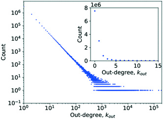 | ||
| Fig. 3 A histogram plot for the out-degree of the limonene network. The inset in the image is a subplot showing a magnification for the degree range from k = 0 to k = 15. | ||
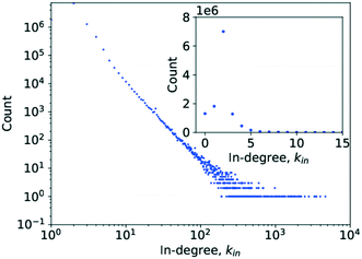 | ||
| Fig. 4 A histogram plot for the in-degree of the limonene network. The inset in the image is a subplot showing a magnification for the degree range from k = 0 to k = 15. | ||
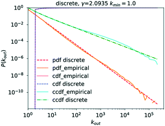
In the case of the out-degree, kout, γout was estimated to be γout ≈ 2.1, which produces good agreement between the data and the model (see Fig. 5). This also agrees well with the values from the literature.4,6
Table 2 shows the R values normalised by their standard deviations along with the p-value of each R value. For several large values of R, the p-value is zero. This is most likely caused by the p-value being so small as to be rounded to zero by the software, as might be expected if the normalised R value deviates greatly from zero. The only distribution scoring a negative log-likelihood ratio in Table 2 is that of the truncated power law which, in addition, scores a very large p-value. Consequently, neither distribution provides a significantly stronger fit for the data analysed. This means that the observed data does indeed follow a power law for very large parts, though the possibility of a truncated tail does exist, which is a feature of many real networks exhibiting scale-free behaviour.25,28,30,52,70,71 This would confirm the network being as a scale-free network.
| Candidate distribution 1 | Candidate distribution 2 | R | p |
|---|---|---|---|
| Power law | Lognormal | 80 | 0.00 |
| Power law | Exponential | 153 | 0.00 |
| Power law | Truncated power law | 0 | 0.92 |
| Power law | Stretched exponential | 19 | 4.18 × 10−81 |
| Power law | Lognormal positive | 287 | 0.00 |
In the case of the in-degree, kin, the picture is more complicated. Grzybowski et al. reported a γin of 2.7, though as evidence only show a degree histogram with a line following a power law with a degree exponent of 2.7 drawn through it.6 The absence of a line of best fit to the actual probability distribution, contrary to what is claimed, and of a cdf complicates verification of the claimed goodness of fit.
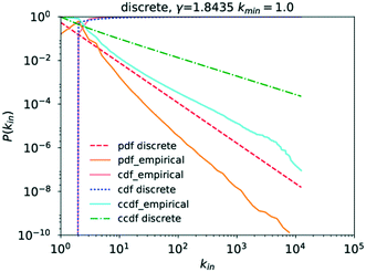
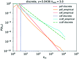
Running a parameter estimation using a power law returns a value of kin ≈ 1.8 which, as can be seen in Fig. 6, produces a very poor fit. Setting kmin at higher values produces better fits as can be seen in Fig. 7 where kmin = 3 produces the best fit and yields γin = 3.0 (the plots for kmin values of 2, 4, 5, and 6 can be found in the ESI† under Fig. S1 through S4). Closer observation of the raw data, particularly the inset in Fig. 4, reveals that the data deviates significantly from the trend expected in a power law in that an in-degree of 2 is significantly more likely to occur than any other degree. More precisely, there are 6![[thin space (1/6-em)]](https://www.rsc.org/images/entities/char_2009.gif) 866
866![[thin space (1/6-em)]](https://www.rsc.org/images/entities/char_2009.gif) 586 nodes with an in-degree of 2 but only 1
586 nodes with an in-degree of 2 but only 1![[thin space (1/6-em)]](https://www.rsc.org/images/entities/char_2009.gif) 770
770![[thin space (1/6-em)]](https://www.rsc.org/images/entities/char_2009.gif) 420 with an in-degree of 1. This deviation from the straight line at kin = 2 can also be observed in the literature data.6 This is caused by reactions being far more likely to involve two reactants than to involve only one. As a consequence, the points for kin = 1 and kin = 0 obscure the power-law trend of the rest of the data.
420 with an in-degree of 1. This deviation from the straight line at kin = 2 can also be observed in the literature data.6 This is caused by reactions being far more likely to involve two reactants than to involve only one. As a consequence, the points for kin = 1 and kin = 0 obscure the power-law trend of the rest of the data.
Analysing the goodness of fit of the power law to the data for kmin = 3 compared to that obtained using the same candidate distributions as those for kout previously, it becomes apparent that P(kin) similarly follows a power law, as can be seen in Table 3, though the option of the truncated power law, statistically speaking, remains here too.
| Candidate distribution 1 | Candidate distribution 2 | R | p |
|---|---|---|---|
| Power law | Lognormal | 104 | 0.00 |
| Power law | Exponential | 78 | 0.00 |
| Power law | Truncated power law | 0 | 0.95 |
| Power law | Stretched exponential | 18 | 2.61 × 10−69 |
| Power law | Lognormal positive | 95 | 0.00 |
Analysing the data on the degree distribution of the chemical network, it is apparent that it does indeed follow a power law and that the power-law exponents are γout ≈ 2.1 and γin ≈ 3. The data on the degree distribution does support the conclusion of the network being scale-free, presented in the literature, even though the in-degree exponent found here deviates from the literature data. Scale-free networks evolve according to a process called “preferential attachment” which means that a node's likelihood to form a new link in the future is directly proportional to its degree.23,27 Therefore, if the network is indeed scale-free, chemical species that partake in a large number of reactions are likely to continue growing more quickly than other species causing the formation of hubs and the core–periphery structure observed for scale-free networks. The significance of the fact that the chemical reaction network conforms to the structure of a general scale-free network is that it follows well-defined evolutionary patterns allowing their use to make predictions about its further, average growth.6,23 It also means that due to the existence of hubs, distances between two molecules in the network are significantly reduced, a fact that is of crucial importance in our use of synthetic chemistry.30 Scale-free networks also represent a very well-investigated class of networks, providing a wealth of possible comparisons to other networks and a large corpus of methods and theories that could be applied to and tested on this network.
4.2. Assortativity
Looking at the results in Tables 4 and 5, it can be observed that the choice of whether or not to include parallel edges turns the network from an assortative to a disassortative network, respectively. In both cases, the absolute magnitude of r is statistically significant but very small, tending towards zero. This indicates that no very strong structure exists to the mixing patterns.| Degree type | r | σ |
|---|---|---|
| Out | 0.009008 | 0.000197 |
| In | 0.070432 | 0.000346 |
| Undirected (in + out) | 0.011679 | 0.000203 |
| Degree type | r | σ |
|---|---|---|
| Out | −0.0121 | 0.000082 |
| In | −0.00783 | 0.000115 |
| Undirected (in + out) | −0.01269 | 0.000081 |
The choice of whether to register multiple instances of the same reaction separately thus clearly matters. Doing so essentially records different ways of carrying out the same reaction. This is very useful information. However, the entire chemical space has not been explored, and even in cases where a reaction has been explored exhaustively, the choice of which set of experiments to register separately is arbitrary. What is of interest in this analysis is the overall connectivity between molecules. Including multiple edges for some of the reactions and not for others would skew this picture, as can be seen in Tables 4 and 5, thus it was decided to register each reaction only once for this part of the work.
Therefore, by examining the results in Table 5, it can be concluded that the Network of Organic Chemistry, in this wiring scheme, exhibits disassortative mixing and thus seems to conform to the trends of biological and technological networks observed in the literature.23,47 Though it must be borne in mind that this is heavily influenced by the wiring scheme. Since the assortativity coefficient can vary from −1 to 1, with a value of 0 indicating no structure to the mixing pattern, it is clear that a value of −0.008 for the in-degree and −0.012 for the out-degree only marginally deviates from zero, leading to the conclusion that the mixing structure observed is very weak and only marginally disassortative.
In terms of chemical interpretations, this implies that, when considering only the connectivity, molecules seem to exhibit little preference as to whether to connect to a hub or a molecule in the periphery. In fact, when considering only the degrees as a metric, there is little structure to the connectivity apparent at all, meaning that a highly versatile platform molecule, for example, is just as likely to react into a highly specialised molecule as it is to yield another platform molecule. This of course is an average metric and when using an average across some 12 million species to try and condense their reactivity trends into a single figure, one might be not surprised to find that the results show very few trends. Indeed, it is the case here that the average hides processes going on within subsections of the chemical space, as will be shown in the following section. However, it was very useful in determining a coherent approach to dealing with multiple instances of the same reaction in the network.
4.3. Degree correlation
Examining Fig. 8 in detail, the observed trend for the correlation between out-degrees seems to be separated into roughly two regions. Firstly, there is a region relatively independent of k, which roughly coincides with the area to the left and above of the x–y diagonal in which low degree nodes connect to higher degree nodes.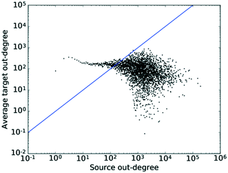 | ||
| Fig. 8 The average degree of the nearest neighbours for all nodes of degree k across all values of k for the out-degrees. The straight line shows the x–y diagonal. | ||
What is observed here most likely is the conversion of feedstocks, which are more specialised and thus have a lower connectivity, into highly connected platform molecules. This would explain the connectivity of the less connected nodes to the more connected ones.
To the right of the x–y diagonal, we observe a high degree of scattering. The reason for this is two-fold. On the one hand, this region lies in the tail of the degree distribution and thus, due to the smaller number of nodes with high degree counts, sees a higher degree of noise. On the other hand, this region maps two processes taking place: (1) the conversion of highly connected platform molecules to other, also highly connected, platform molecules, i.e. the conversion of intermediates into intermediates along a synthesis route, and (2) the conversion of highly connected platform molecules into specialised products with a resulting lower degree count, which is a disassortative mixing process. Seeing as the majority of nodes lie in the low degree region, where the correlation is independent of k, this results in an assortativity coefficient close to 0, while the region exhibiting the disassortative scattering would result in a slightly negative value. Thus, the plot matches the pattern expected from theory. Furthermore, the existence of these separate regions and the different functions fulfilled by different nodes also indicates the likely existence of some degree of hierarchy amongst the nodes.
The pattern in Fig. 9 shows very little correlation to k. Given an in-degree assortativity coefficient value of −0.0078 found in the previous section, this matches the trend expected, or rather the absence thereof, very well. The tail of the distribution again exhibits some degree of scattering, which would also be expected due to the signal-to-noise ratio deteriorating as the number of nodes in that region decreases. This plot confirms the results obtained when calculating the assortativity coefficient, namely that no significant degree correlation exists for the in-degree.
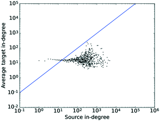 | ||
| Fig. 9 The average degree of the nearest neighbours for all nodes of degree k across all values of k for the in-degrees. The straight line shows the x–y diagonal. | ||
Taking the results of this section and the preceding section on “Assortativity” together, the conclusion of a mildly disassortative network with little mixing structure in large parts is supported by investigating both the assortativity coefficient and the degree correlation, while also providing some indication of the existence of a hierarchical structure within the network.
4.4. Average shortest path length
As can be seen from Fig. 10, the value of P(![[small script l]](https://www.rsc.org/images/entities/i_char_e146.gif) ) peaks at a value of 5, though due to the number of longer paths the average is skewed to the right of this. The average shortest path length of the network in the year 2016 is 6.02. On logarithmic axes (Fig. 10), it becomes apparent that this shift is caused by a small peak for a path length falling between
) peaks at a value of 5, though due to the number of longer paths the average is skewed to the right of this. The average shortest path length of the network in the year 2016 is 6.02. On logarithmic axes (Fig. 10), it becomes apparent that this shift is caused by a small peak for a path length falling between ![[small script l]](https://www.rsc.org/images/entities/i_char_e146.gif) = 50 and
= 50 and ![[small script l]](https://www.rsc.org/images/entities/i_char_e146.gif) = 60, most likely caused by the existence of a poorly connected set of molecules in an island in the network.
= 60, most likely caused by the existence of a poorly connected set of molecules in an island in the network.
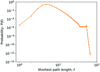 | ||
Fig. 10 Probability distribution of the shortest path length, P(![[small script l]](https://www.rsc.org/images/entities/i_char_e146.gif) ), plotted against the shortest path length, ), plotted against the shortest path length, ![[small script l]](https://www.rsc.org/images/entities/i_char_e146.gif) , on logarithmic axes. The data points have been marked by dark orange dots. , on logarithmic axes. The data points have been marked by dark orange dots. | ||
This value of  means that it is possible to synthesise any species out of any other species, on average, within a maximum of six synthesis steps, which might be perceived as a surprisingly small number though the parallel to the “six degrees of separation” observed by Milgram in social networks is immediately apparent.55,56
In order to investigate the existence of a small world effect more closely, the results of the analysis of the variation of  with the number of nodes in the network were plotted and are shown in Fig. 11.
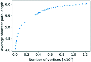 | ||
| Fig. 11 The average shortest path length for a given network size against the number of nodes of that network size. | ||
When replotting Fig. 11 using a logarithmic scale the average shortest path length does scale logarithmically with respect to the number of nodes, while even obeying a proportionality with log![[thin space (1/6-em)]](https://www.rsc.org/images/entities/char_2009.gif) log
log![[thin space (1/6-em)]](https://www.rsc.org/images/entities/char_2009.gif) N, a supposed hallmark of scale-free networks with degree exponents 2 ≤ γ ≤ 3,23,30 as can be seen in Fig. S7 and S8 in the ESI,† respectively. However, there exists ambiguity about the precise scaling relationship for networks with power-law distributions.18
N, a supposed hallmark of scale-free networks with degree exponents 2 ≤ γ ≤ 3,23,30 as can be seen in Fig. S7 and S8 in the ESI,† respectively. However, there exists ambiguity about the precise scaling relationship for networks with power-law distributions.18
It can therefore be concluded that the Network of Organic Chemistry, as investigated here, does indeed display a “small world” effect. Though very interesting in giving information about the topology of the network, the small world effect tells us little about the organising principle of a given network as, for example, random networks can display this property too.25 The importance of this property, however, is illustrated by the fact that if the Network of Organic Chemistry were, for example, organised as a grid, the average shortest path length would scale with the square root of the number of chemical species registered, thus greatly increasing the number of reactions required to synthesise a species, on average. Though as an average the path length of 5–6 steps does not provide a hard-and-fast criterion for synthetic efficiency, it might serve as a point of comparison when designing a new synthesis route. A route significantly deviating from this figure significantly deviates from the average, meaning that, unless the synthesis is in a highly specialised niche, potential for a shorter route might exist. The analysis of the degree correlation above also suggested that synthetic routes quickly move through a few well-connected ‘hub’ molecules towards the more specialised end-molecules, which is what appears to have been confirmed here, represented by the relatively short lengths of most routes.
4.5. Clustering coefficient
In the case of the network under investigation, the global clustering coefficient is 0.00058 with a standard deviation of 8.61 × 10⁻⁵. For many real-world networks, the value ranges between 0.01 and 0.5,57,72 making this a network showing a very low degree of clustering.For some scale-free networks, power-law behaviour is evidenced for ![[c with combining overline]](https://www.rsc.org/images/entities/i_char_0063_0305.gif) (k) in that
(k) in that ![[c with combining overline]](https://www.rsc.org/images/entities/i_char_0063_0305.gif) (k) ∝ k−1.18,52 In a number of publications by other authors, it is shown that this is a characteristic of hierarchical networks,23,32,37,40,42,44 which can be considered a sub-class of scale-free networks, though Soffer and Vázquez presented some evidence that this trend could arise out of the existence of degree correlations which shows up as a consequence of how the clustering coefficient is defined.24 Following the initial argument, however, this scaling relationship provides a quantitative indicator of the existence of a hierarchy of nodes with different degrees of modularity.37 Specifically, this behaviour is caused by low-degree vertices forming small, internally well-connected sub-communities (which gives rise to a high clustering coefficient), linking out to high-degree hubs which only have few edges connecting them to the many sub-graphs that they link to and thus have a low clustering coefficient.23,42,44
(k) ∝ k−1.18,52 In a number of publications by other authors, it is shown that this is a characteristic of hierarchical networks,23,32,37,40,42,44 which can be considered a sub-class of scale-free networks, though Soffer and Vázquez presented some evidence that this trend could arise out of the existence of degree correlations which shows up as a consequence of how the clustering coefficient is defined.24 Following the initial argument, however, this scaling relationship provides a quantitative indicator of the existence of a hierarchy of nodes with different degrees of modularity.37 Specifically, this behaviour is caused by low-degree vertices forming small, internally well-connected sub-communities (which gives rise to a high clustering coefficient), linking out to high-degree hubs which only have few edges connecting them to the many sub-graphs that they link to and thus have a low clustering coefficient.23,42,44
The results of calculating the degree-dependent average clustering coefficient have been plotted in Fig. 12. It is easily apparent that ![[c with combining overline]](https://www.rsc.org/images/entities/i_char_0063_0305.gif) (k) approximately follows a proportionality to k−1 too, which would be evidence of a hierarchical network.23 The clustering coefficient for k = 2 and k = 3 exhibits a visible deviation from the rest of the trend. The reason for this is that these nodes in most cases will represent highly specialised substances participating in very few reactions and thus residing in the periphery of the core–periphery structure of a scale-free network, which leads to a lower clustering coefficient and, consequently, a decrease of the average clustering coefficient for the concerned degree classes.
(k) approximately follows a proportionality to k−1 too, which would be evidence of a hierarchical network.23 The clustering coefficient for k = 2 and k = 3 exhibits a visible deviation from the rest of the trend. The reason for this is that these nodes in most cases will represent highly specialised substances participating in very few reactions and thus residing in the periphery of the core–periphery structure of a scale-free network, which leads to a lower clustering coefficient and, consequently, a decrease of the average clustering coefficient for the concerned degree classes.
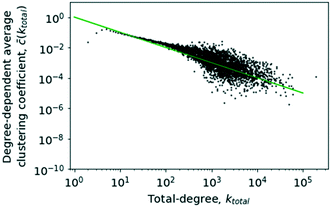 | ||
| Fig. 12 The degree-dependent average clustering coefficient against the total degree, k. The solid line shows a plot of k−1 for comparison. | ||
As given in Fig. 12, it can be concluded that the network does follow the trend expected of a hierarchical network reinforcing the conclusions about a hierarchical network architecture.
4.6. Betweenness centrality
The central point dominance of the network was found to be 0.003719. This would indicate that despite the existence of hub molecules, the wiring of the network is very decentralised, not necessarily relying on central hubs in order to navigate the network. As seen from the definition in eqn (14), this is an average property and, given the size of the network, may hide significant deviations. In the following, results of the betweenness centrality analysis are given. Unlike the values used to calculate the central point dominance, the values given subsequently have not been normalised.Goh et al. observed that though the degree distribution of a scale-free network does follow a power law, with an exponent in most cases of 2 ≤ γ ≤ 3, the exact value varies without being able to precisely classify why. Goh et al., however, observed that in scale-free networks, the betweenness distribution follows a power law too. The exponent of this power law took one of two values, either η ≈ 2.2 or η ≈ 2.0. With this, Goh et al. had a more precise metric for characterising a given scale-free network which led to their characterisation of class I or class II scale-free networks based on the value of the power-law exponent of the betweenness distribution.73 These findings are similarly supported in ref. 52 where Pastor-Satorras and Vespignani reported that certain layers of the internet exhibit a power-law distribution in the betweenness centrality. This distribution, however, truncates for high betweenness values.
As is clearly visible when plotting the vertex betweenness centrality for the network under investigation, this is not straightforwardly the case here. Examining Fig. 13, it becomes apparent that at least three regions are present. Firstly, below a betweenness value of 1, the probability of observing a given betweenness is constant. The plot then enters a second regime, visually obeying a power-law trend. Between 5 × 10⁵ and roughly 5 × 10⁷, the curve enters what might be considered a transition region marked by large fluctuations in the probability values, before finally settling back into what resembles a power law by visual inspection before finally exhibiting further fluctuations due to the heavy tail. The observations of discrete regions might be caused by the already observed difference in degree distributions for the in- and out-degrees combined with the fact that the out-degrees observed exhibit a greater range of values while the in-degrees, generally, have a smaller magnitude as can be seen in Fig. 3 and 4. Thus, as high degree nodes become more important in the observed phenomena, a different distribution would be expected to start dominating, leading to a different regime.
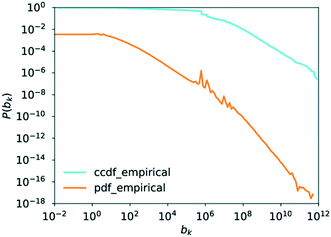 | ||
| Fig. 13 The probability density function and the complementary cumulative distribution function of the betweenness centrality plotted against the betweenness centrality. | ||
Examining the regions more closely, it becomes apparent that there are indeed two separate phenomena at play, which was also observed for some layers of the internet.52 The first regime, when analysing 1.0 ≤ bk ≤ 5 × 10⁵, has a reasonable fit for a power law with γ ≈ 1.14 as seen in Fig. S5 in the ESI.† Analysing the results of the statistical evaluation of the goodness of fit compared to other candidate distributions (following the same procedure as outlined in the Methodology section for “Degree Distribution”), which can be found in Table 6, it becomes apparent that the fit is very poor, providing only a better description than the exponential distribution of all the distributions tested. This means that it is impossible to conclude that the data observed follows a power law in this region.
| Candidate distribution 1 | Candidate distribution 2 | R | p |
|---|---|---|---|
| Power law | Lognormal | −892 | 0.00 |
| Power law | Exponential | 595 | 0.00 |
| Power law | Truncated power law | −1523 | 0.00 |
| Power law | Stretched exponential | −950 | 0.00 |
| Power law | Lognormal positive | −892 | 0.00 |
The predicted value for γ appears much better, and in line with literature expectations, at γ ≈ 1.97, when considering the other regime with 5 × 10⁷ ≤ bk as is seen in Fig. S6 in the ESI.† This would agree well with the findings quoted in ref. 73. If the ability of a power law to describe the trend is compared to that of other possible distributions, the picture is much less clear, however. Considering the results of this analysis, shown in Table 7, it can be noted that the power law provides an ability to describe the data better than the exponential distribution can, which is statistically significant. Though the R-value of the comparison to the stretched exponential distribution favours the latter, the p-value of 0.07 renders the comparison potentially inconclusive. The truncated power law provides a seemingly better description than the power-law distribution. This result, however, does not necessarily conflict with the claim of the distribution exhibiting a power-law behaviour, as the distribution is truncated. The fact that the lognormal distribution, as well as the positive lognormal distribution, describes the data better would cast doubt on the existence of a heavy tail. This could, however, be a consequence of the distribution being fitted to the tail end of the overall distribution.
| Candidate distribution 1 | Candidate distribution 2 | R | p |
|---|---|---|---|
| Power law | Lognormal | −8 | 5.59 × 10⁻¹⁶ |
| Power law | Exponential | 16 | 9.73 × 10−55 |
| Power law | Truncated power law | −2 | 1.55 × 10−06 |
| Power law | Stretched exponential | −2 | 0.07 |
| Power law | Lognormal positive | −8 | 5.59 × 10⁻¹⁶ |
As a consequence of these data, it is concluded that the investigated network's vertex betweenness centrality probability distribution does not obey a straightforward power law. It seems as if different regimes can be observed. Analysing these regimes in turn leads to partially inconclusive results unable to verify the hypothesis that the network's scale-free behaviour manifests itself in the betweenness centrality distribution as well as in the degree distribution. A potential cause for this could lie in the different behaviour of the incoming edges compared to the outgoing edges already observed during the analysis of the degree distribution and in their mixing behaviour.
Examining Fig. 14, as well as Fig. 15, it can be seen that there is a very clear, positive correlation between the degree and the average betweenness centrality of those nodes, for both the in- and the out-degree. In chemistry terms, this would support the hypothesis that not only do the central, highly connected hub molecules combine a large number of connections upon themselves but also a large share of the geodesics in the network. Thus the load appears to run via them and a vast majority of synthesis routes would go through a small number of very important hub molecules. Given this, a very clear hierarchy can be observed in the nodes of the network. Though there is no indication for the existence of distinct hierarchies, there clearly is a fluid hierarchy of nodes. Very interestingly, this matches precisely the findings of Pastor-Satorras and Vespignani for the internet.52 As the current network evolved largely from petrochemical syntheses, it may be an interesting research question if the increased use of bio-feedstocks and rapid development of novel transformations of bio-feedstocks would lead to a significantly different structure of the network with new hub molecules.
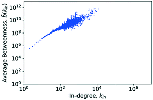 | ||
| Fig. 14 The average degree-dependent betweenness calculated for the in-degree against the in-degree. The error bars show the standard deviation of the data associated with each average. | ||
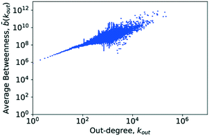 | ||
| Fig. 15 The average degree-dependent betweenness calculated for the out-degree against the out-degree. The error bars show the standard deviation of the data associated with each average. To summarise this section, a brief overview of the results of each of the metrics is given in Table 8. | ||
| Metric | Finding |
|---|---|
| Degree distribution | Largely scale-free behaviour |
| Assortativity | Very mild disassortativity |
| Degree correlation | Very mild disassortativity |
| Average shortest path length | Small-world, on average six steps |
| Clustering | Power-law dependence on degree |
| Betweenness centrality | Apparent hierarchy of nodes |
Conclusions
A number of key graph theoretical properties of this network were analysed. The Introduction has presented an overview of some of the types of networks studied in the literature. In Results and discussion under “Degree distribution”, the analysis of the degree distribution is given along with the degree histogram for the nodes of the network and the sections on “Assortativity” and “Degree correlation” show results on the assortativity of the network and the degree correlation between nodes. The results section on “Average shortest path length” has looked at the change in average shortest path lengths as the network grows as well as the probability distribution of observing a given path length. Also in Results and discussion, the section on the “Clustering coefficient” looked at the degree-dependent clustering coefficient before concluding the results with the degree-dependent betweenness centrality in “Betweenness centrality”.An important conclusion from the results section on “Degree distribution” is that the in-degree distribution is offset and deviates from a power law for degrees less than two which can also be observed in the literature on the topic.4,6 Regardless, a statistically validated trend fitting a power law could be ascertained for both distributions with γin ≈ 3 and γout ≈ 2.1. Though the value for γin deviates from that reported in the literature, it is possible to conclude that the network is indeed scale-free in nature confirming what has been reported previously.4,6
The results section on “Assortativity” was able to provide important evidence for the effect that parallel edges have on some of the network dynamics involved. This revolves around the question whether to register the same reaction reported separately under different conditions as one reaction or as separate instances. Not permitting parallel edges, and thus registering each reaction only once regardless of conditions, was seen as the most consistent approach which thus meant that the network was very slightly disassortative. This finding was supported by the results section on “Degree correlation” which also provided evidence for a hierarchical network architecture. Neither property has been investigated for the NOC in the literature previously.
Analysis of the network's average shortest path length's dependence on the number of nodes in this network was able to show that the NOC exhibited a “small world effect” which, through its short path lengths, provides further indications of a possible hierarchical architecture. In addition, the analysis of the average shortest path length showed that the network of organic chemistry resembled the six degrees of separation observed in Milgram's seminal paper on social networks. The clear power-law proportionality between the degree-dependent average clustering coefficient, c, and the degree also showed that the nodes of the network exhibit a very fluid hierarchical structure. Both of these represent interesting new findings.
This evidence for a hierarchy of nodes was finally most clearly confirmed in Fig. 14 and 15 in the results section for “Betweenness centrality” analysing the betweenness values observed in the network, which had not been done on the NOC prior to this. This data showed very clearly that the hub molecules do not only combine a large share of connections upon themselves, as identified as part of the scale-free model already, but seemingly also carry a large share of the “load” of the network, clearly indicating that a hierarchy of nodes exists and manifests itself in a number of ways.
It can be observed that several key network metrics seem to indicate a hierarchy, even if fluid, of nodes across the range of their parameter space while showing some of the hallmark characteristics set out in the literature for hierarchical networks. Therefore there is evidence supporting the conclusion that the Network of Organic Chemistry, as observed here, not only is scale-free but also displays a hierarchical architecture which represents a novel finding about the architecture of chemistry.
In answer to the question at the outset of this paper, it can thus be noted that the network not only is indeed scale-free, but also exhibits small world behaviour while furthermore providing evidence of a hierarchy of nodes in its topology.
Studying the statistical properties of the network has yielded a number of insights into the statistical behaviour of the network of organic reactions. The finding that the known chemical space organises into a scale-free network means that it is possible to, on average, predict how the number of reactions that a given chemical species participates in will evolve as new reactions are discovered in the future. At the same time, it has been found that the existence of hub molecules caused by this evolutionary behaviour positively impacts many properties of the network, for example, by allowing to find shorter pathways and reducing the minimum number of steps required to carry out a synthesis. Thus, it was shown that most syntheses can, on average, be performed in 6 steps. It was also possible to identify the differing behaviour of platform molecules and feedstocks as well as specialised products in the mixing structure of the network. Finally, the suspected hierarchical structure leads to the fact that the hub molecules not only combine a large number of reactions onto them but also are crucial in being involved in a large number of synthesis routes.
Conflicts of interest
There are no conflicts to declare.Acknowledgements
P.-M. Jacob would like to thank Peterhouse and the University of Cambridge for funding in the form of a PhD studentship. We gratefully acknowledge collaboration with RELX Intellectual Properties SA and their technical support, which enabled us to mine Reaxys. This work was funded, in part, by the EPSRC project “Terpene-based manufacturing for sustainable chemical feedstocks” EP/K014889.References
-
Elsevier R&D Solutions, Reaxys Fact Sheet, https://www.elsevier.com/__data/assets/pdf_file/0005/91616/RDS_FactSheet_Reaxys_Oct_2016-WEB.pdf, (accessed 27 February 2017) Search PubMed
.
- RELX Intellectual Properties SA, Reaxys - Reaxys is a trademark, copyright owned by RELX Intellectual Properties SA and used under licence., https://www.reaxys.com/, (accessed 8 February 2017)
.
-
O. Ravitz, Wiley ChemPlanner - Technical Notes, http://images.news.wiley.com/Web/WileyEnterprise/%7B84e34101-2105-40fd-8d3a-df6120ebf89e%7D_Info-RC-CHE-W2627_ChemPlanner_Technical_Notes.pdf, (accessed 20 May 2016) Search PubMed
.
- M. Fialkowski, K. J. M. Bishop, V. A. Chubukov, C. J. Campbell and B. A. Grzybowski, Angew. Chem., Int. Ed., 2005, 44, 7263–7269 CrossRef CAS PubMed
.
- K. J. M. Bishop, R. Klajn and B. A. Grzybowski, Angew. Chem., Int. Ed., 2006, 45, 5348–5354 CrossRef CAS PubMed
.
- B. A. Grzybowski, K. J. M. Bishop, B. Kowalczyk and C. E. Wilmer, Nat. Chem., 2009, 1, 31–36 CrossRef CAS PubMed
.
- P. E. Fuller, C. M. Gothard, N. A. Gothard, A. Weckiewicz and B. A. Grzybowski, Angew. Chem., 2012, 124, 8057–8061 CrossRef
.
- C. M. Gothard, S. Soh, N. A. Gothard, B. Kowalczyk, Y. Wei, B. Baytekin and B. A. Grzybowski, Angew. Chem., 2012, 124, 8046–8051 CrossRef
.
- S. Soh, Y. Wei, B. Kowalczyk, C. M. Gothard, B. Baytekin, N. A. Gothard and B. A. Grzybowski, Chem. Sci., 2012, 3, 1497 RSC
.
- M. Kowalik, C. M. Gothard, A. M. Drews, N. A. Gothard, A. Weckiewicz, P. E. Fuller, B. A. Grzybowski and K. J. M. Bishop, Angew. Chem., Int. Ed., 2012, 51, 7928–7932 CrossRef CAS PubMed
.
- S. Szymkuc, E. P. Gajewska, T. Klucznik, K. Molga, P. Dittwald, M. Startek, M. Bajczyk and B. A. Grzybowski, Angew. Chem., Int. Ed., 2016, 55, 5904–5937 CrossRef CAS PubMed
.
- A. A. Lapkin, P. K. Heer, P.-M. Jacob, M. Hutchby, W. Cunningham, S. D. Bull and M. G. Davidson, Faraday Discuss., 2017, 202, 483–496 RSC
.
- P.-M. Jacob, P. Yamin, C. Perez-Storey, M. Hopgood and A. A. Lapkin, Green Chem., 2017, 19, 140–152 RSC
.
- E. J. Corey and W. T. Wipke, Science, 1969, 166, 178–192 CAS
.
- E. Bullmore and O. Sporns, Nat. Rev. Neurosci., 2009, 10, 186–198 CrossRef CAS PubMed
.
-
G. Caldarelli, Scale-Free Networks - Complex Webs in Nature and Technology, Oxford University Press, Oxford, 2007 Search PubMed
.
- L. D. F. Costa, F. A. Rodrigues, G. Travieso and P. R. Villas Boas, Adv. Phys., 2007, 56, 167–242 CrossRef
.
- M. E. J. Newman, SIAM Rev., 2003, 45, 167–256 CrossRef
.
- R. Ahnert and S. E. Ahnert, Leonardo, 2014, 47, 275 CrossRef
.
- R. Ahnert and S. E. Ahnert, ELH, 2015, 82, 1 CrossRef
.
- M. Dehmer and F. Emmert-Streib, IEE Proc.: Syst. Biol., 2011, 5, 185–207 Search PubMed
.
-
P. Erdös and A. Rényi, Publ. Math. Inst. Hungarian Acad. Sci., 1960, vol. 5, pp. 17–61 Search PubMed
.
- A.-L. Barabasi and Z. N. Oltvai, Nat. Rev. Genet., 2004, 5, 101–113 CrossRef CAS PubMed
.
- S. N. Soffer and A. Vázquez, Phys. Rev. E: Stat., Nonlinear, Soft Matter Phys., 2005, 71, 57101 CrossRef PubMed
.
- R. Albert and A.-L. Barabási, Rev. Mod. Phys., 2002, 74, 47–97 CrossRef
.
- D. J. de Solla Price, Science, 1965, 149, 510–515 CAS
.
- A.-L. Barabási and R. Albert, Science, 1999, 286, 509–512 CrossRef
.
- S. H. Strogatz, Nature, 2001, 410, 268–276 CrossRef CAS PubMed
.
- T. Zhou, G. Yan and B.-H. Wang, Phys. Rev. E: Stat., Nonlinear, Soft Matter Phys., 2005, 71, 46141 CrossRef PubMed
.
- S. Boccalletti, V. Latora, Y. Moreno, M. Chavez and D. Hwang, Phys. Rep., 2006, 424, 175–308 CrossRef
.
-
X. F. Wang and G. Chen, IEEE Circuits Syst. Mag., 2003, vol. 3, pp. 6–20 Search PubMed
.
- E. Ravasz and A.-L. Barabási, Phys. Rev. E: Stat., Nonlinear, Soft Matter Phys., 2003, 67, 26112 CrossRef PubMed
.
- G. Bardella, A. Bifone, A. Gabrielli, A. Gozzi and T. Squartini, Sci. Rep., 2016, 6, 32060 CrossRef CAS PubMed
.
- D. Meunier, R. Lambiotte and E. T. Bullmore, Front. Neurosci., 2010, 4, 1–11 Search PubMed
.
- A. Clauset, C. Moore and M. E. J. Newman, Nature, 2008, 453, 98–101 CrossRef CAS PubMed
.
- M. Sales-Pardo, R. Guimera, A. A. Moreira and L. A. N. Amaral, Proc. Natl. Acad. Sci. U. S. A., 2007, 104, 15224–15229 CrossRef CAS PubMed
.
- E. Ravasz, Science, 2002, 297, 1551–1555 CrossRef CAS PubMed
.
- A. Clauset, C. Moore and M. E. J. Newman, Nature, 2008, 453, 98–101 CrossRef CAS PubMed
.
- J. Noh, Phys. Rev. E: Stat., Nonlinear, Soft Matter Phys., 2003, 67, 45103 CrossRef PubMed
.
- S. Fortunato, Phys. Rep., 2010, 486, 75–174 CrossRef
.
- O. Mason and M. Verwoerd, IET Syst. Biol., 2007, 1, 89–119 CrossRef CAS PubMed
.
- A. Barrat, M. Barthelemy, R. Pastor-Satorras and A. Vespignani, Proc. Natl. Acad. Sci. U. S. A., 2004, 101, 3747–3752 CrossRef CAS PubMed
.
- M. Rubinov and O. Sporns, Neuroimage, 2010, 52, 1059–1069 CrossRef PubMed
.
- A. Vázquez, Phys. Rev. E: Stat., Nonlinear, Soft Matter Phys., 2003, 67, 56104 CrossRef PubMed
.
- B. Barzel and A.-L. Barabási, Nat. Phys., 2013, 9, 673–681 CrossRef CAS PubMed
.
- A. Arcagni, R. Grassi, S. Stefani and A. Torriero, arXiv Prepr. arXiv1602.03650, 2016, p. 24 Search PubMed.
- M. E. J. Newman, Phys. Rev. E: Stat., Nonlinear, Soft Matter Phys., 2003, 67, 26126 CrossRef CAS PubMed
.
- M. Piraveenan, M. Prokopenko and A. Zomaya, IEEE/ACM Trans. Comput. Biol. Bioinf., 2012, 9, 66–78 CrossRef PubMed
.
- D. B. Larremore, A. Clauset and A. Z. Jacobs, Phys. Rev. E: Stat., Nonlinear, Soft Matter Phys., 2014, 90, 12805 CrossRef PubMed
.
- M. E. J. Newman and J. Park, Phys. Rev. E: Stat., Nonlinear, Soft Matter Phys., 2003, 68, 36122 CrossRef CAS PubMed
.
- R. Pastor-Satorras, A. Vázquez and A. Vespignani, Phys. Rev. Lett., 2001, 87, 258701 CrossRef CAS PubMed
.
-
R. Pastor-Satorras and A. Vespignani, in Evolution and Structure of the Internet, ed. W. N. Adger and A. Jordan, Cambridge University Press, Cambridge, 2004, pp. 36–68 Search PubMed
.
-
A. Bonato and F. Chung, in Handbook
of Graph Theory, ed. J. L. Gross, J. Yellen and P. Zhang, CRC Press/Taylor and Francis, Boca Raton, FL, 2nd edn., 2014, pp. 1456–1476 Search PubMed
.
-
E. Estrada, in The Structure of Complex Networks - Theory and Application, Oxford University Press, Oxford, 1st edn., 2012, pp. 47–72 Search PubMed
.
- S. Milgram, Psychol. Today, 1967, 60–67 Search PubMed
.
- J. Travers and S. Milgram, Sociometry, 1969, 32, 425 CrossRef
.
- M. Girvan and M. E. J. Newman, Proc. Natl. Acad. Sci. U. S. A., 2002, 99, 7821–7826 CrossRef CAS PubMed
.
- M. Ángeles Serrano and M. Boguñá, Phys. Rev. E: Stat., Nonlinear, Soft Matter Phys., 2005, 72, 36133 CrossRef PubMed
.
- D. J. Watts and S. H. Strogatz, Nature, 1998, 393, 440–442 CrossRef CAS PubMed
.
- T. P. Peixoto, figshare DOI:10.6084/m9.figshare.1164194
.
-
M. Gjoka, M. Kurant and A. Markopoulou, in 2013 Proceedings IEEE INFOCOM, IEEE, 2013, pp. 1968–1976 Search PubMed
.
- M. Catanzaro, M. Boguñá and R. Pastor-Satorras, Phys. Rev. E: Stat., Nonlinear, Soft Matter Phys., 2005, 71, 27103 CrossRef PubMed
.
- L. C. Freeman, Sociometry, 1977, 40, 35 CrossRef
.
- G. Zamora-López, C. Zhou and J. Kurths, Front. Neuroinform., 2010, 4, 1–13 Search PubMed
.
-
Elsevier R&D Solutions, Reaxys Fact sheet, http://www.elsevier.com/__data/assets/pdf_file/0005/91616/R_D-Solutions_RX_Fact-Sheet_DIGITAL1.pdf, (accessed 20 August 2015) Search PubMed
.
- M. Fialkowski, K. J. M. Bishop, V. A. Chubukov, C. J. Campbell and B. A. Grzybowski, Angew. Chem., Int. Ed., 2005, 44, 7263–7269 CrossRef CAS PubMed
.
- J. Alstott, E. Bullmore and D. Plenz, PLoS One, 2014, 9, e85777 Search PubMed
.
- A. Clauset, C. R. Shalizi and M. E. J. Newman, SIAM Rev., 2009, 51, 661–703 CrossRef
.
-
R. Pastor-Satorras and A. Vespignani, in Evolution and Structure of the Internet, Cambridge University Press, Cambridge, 2004, pp. 240–242 Search PubMed
.
- L. A. N. Amaral, A. Scala, M. Barthelemy and H. E. Stanley, Proc. Natl. Acad. Sci. U. S. A., 2000, 97, 11149–11152 CrossRef CAS PubMed
.
- S. Mossa, M. Barthélémy, H. Eugene Stanley and L. A. Nunes Amaral, Phys. Rev. Lett., 2002, 88, 138701 CrossRef PubMed
.
- M. E. J. Newman, D. J. Watts and S. H. Strogatz, Proc. Natl. Acad. Sci. U. S. A., 2002, 99, 2566–2572 CrossRef PubMed
.
- K.-I. Goh, E. Oh, H. Jeong, B. Kahng and D. Kim, Proc. Natl. Acad. Sci. U. S. A., 2002, 99, 12583–12588 CrossRef CAS PubMed
.
Footnote |
| † Electronic supplementary information (ESI) available. See DOI: 10.1039/c7re00129k |
| This journal is © The Royal Society of Chemistry 2018 |


