 Open Access Article
Creative Commons Attribution 3.0 Unported Licence
A machine learning based approach to reaction rate estimation†
Matthew S.
Johnson
 and
William H.
Green
 *
*
Department of Chemical Engineering, Massachusetts Institute of Technology, Cambridge, MA 02139, USA. E-mail: whgreen@mit.edu
First published on 15th February 2024
Abstract
Chemical kinetic models are vital to accurately predicting phenomena in a wide variety of fields from combustion to atmospheric chemistry to electrochemistry. However, building an accurate chemical kinetic model requires the efficient and accurate estimation of many reaction rate coefficients for many reaction classes with highly variable amounts of available training data. Current techniques for fast automatic rate estimation tend to be poorly optimized and tedious to maintain and extend. We have developed a machine learning algorithm for automatically training subgraph isomorphic decision trees (SIDT) to predict rate coefficients for arbitrary reaction types. This method is fully automatic, scalable to virtually any dataset size, human readable, can incorporate qualitative chemical knowledge from experts and provides detailed uncertainty information for estimates. The accuracy of the algorithm is tested against the state of the art rate rules scheme in the RMG-database for five selected reaction families. The SIDT method is shown to significantly improve estimation accuracy across all reaction families and considered statistics. The estimator uncertainty estimates are validated against actual errors.
1 Introduction
Automatic, rapid and accurate estimation of reaction rates is critical in the development of large chemical kinetic models. Kinetic models can contain tens of thousands of kinetic parameters1 and the construction processes require estimation of many more to decide which reactions are fast enough to be important. Furthermore, chemical kinetic models are only increasing in size requiring estimation of more and more rate coefficients. Rate based automatic mechanism generation relies even more on accurate estimates as the quality of these estimates affects the species and reactions included.2–5While quantum chemistry calculations can be used to estimate reaction rates to high accuracy, they are not fast and not yet fully automatic. Although computers continue to become faster, high accuracy quantum chemistry calculations can take days to weeks to run. Furthermore, there are often difficulties in finding the transition state of a particular reaction, requiring human intervention, making the process even slower.
Much progress is being made on automatic high accuracy rate calculations based on transition state finding algorithms such as Kinbot, nudged elastic band, HFSP, AFIR, and string methods6–12 and workflow codes such as ARC, Pynta, KinBot, and AutoMech.6,9,13,14 However, for the moment these methods are computationally expensive and not entirely robust, with only limited benchmarking.15,16 But even if these methods were robust, it would probably be impractical to use them to compute all the rate coefficients of interest (though perhaps this assessment could change after exascale computers become widely available).
Our group has used these automated methods to construct a large dataset of DFT transition state (TS) geometries17 and a corresponding dataset of CCSD(T) barrier heights.18 These datasets have been used to train machine learning models that provide useful initial guesses at TS geometries19 and estimates of barriers for a certain class of reactions of small closed-shell molecules.20 The neural-net modeling methods we developed for these tasks19,21,22 have some promise, but are still far from perfect; among other problems they require huge training sets of accurate transition states or barriers, and at present the uncertainties in each prediction is unknown. This latter problem is important because even if the average prediction error is acceptably small, a significant percentage of the rate predictions can be completely wrong, with no warning to the user.
Fast accurate kinetics estimation for reaction mechanisms is a difficult problem. Fundamentally, the 2-D structures of the reactants (typical of reaction mechanisms), the atom mapping, the type of reaction and the thermodynamic information for the reactant and product must be mapped to a temperature dependent reaction rate. The problem is very different from thermodynamic property prediction.
Thermodynamic properties typically have very linear relationships with their molecular structures due to the fact that the thermodynamic properties (Hf298, Sf298, Cp(T)) of a molecule are approximately equal to the sum of the thermodynamic contributions of its individual substructures.23 One can try a similar approach to estimate the thermochemistry of transition states,24 but it requires a much larger set of substructures. Unlike thermochemical properties, reactions both have many different types and are much more difficult to calculate. This means that it requires larger datasets to train rate estimation algorithms and the available datasets are much sparser. These properties necessitate particular care when designing algorithms for estimating the rates of chemical reactions.
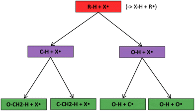
The most traditional approach to quickly estimating reaction rates in mechanism construction is rate rules (RR).2,4,25 Abstractly a rate rule maps all reactions with specific substructures around the atoms participating in the reaction to a specified reaction rate. These substructures for hydrogen abstraction might look something like R–CH2–R*(·)H–CH3 + H*–CH2–R. A reaction is estimated using the rate rule corresponding to the most specific substructures it matches that a rate rule is known for. These rate rules and associated substructures are usually written by hand. The RR system used by the reaction mechanism generator (RMG) software uses an improved version of this that allows use of a set of training reactions.2,4 In this formulation for a given tree structure (see Fig. 1) training reactions descend down the tree (following the substructures they match) and become additional rate rules at the most specific node they match. This allows rules to be generated from training data given a fixed tree structure. The RR approach suffers from two primary disadvantages: (i) the rules must be constructed manually, taking substantial human time and effort to update and improve and (ii) the accuracy of RR depends on the assumed tree structure.
Other approaches have used reaction group additivity.24,26–29 Reaction group additivity works much like thermodynamic group additivity except that instead of adding linear components from specific atoms to estimate thermodynamic parameters linear components are added from specific substructures of the reaction mapping to estimate kinetic parameters. The substructures follow a set of manually written trees for each reaction type and then the contribution to each kinetic parameter at each substructure is fit linearly to a set of reaction rates. Most often the kinetic parameters used are the logarithm of the components of the modified Arrhenius form log(A) + n![[thin space (1/6-em)]](https://www.rsc.org/images/entities/char_2009.gif) log(T) −
log(T) −  , where A, n, Ea are the Arrhenius parameters, R is the gas constant and T is the temperature. The performance of reaction group additivity is in general mixed. When applied to limited regions of chemical space that are well covered with data, good performance can be achieved.24,26,28 However, so far when applied to large chemical spaces where the data is more sparse, such as the training set for RMG's estimators, performance has been poor compared to RR.29 Additionally, reaction group additivity much like RR must be manually formulated and the accuracy is limited by that formulation.
Most recently neural nets, decision trees and genetic algorithms have been applied to predicting kinetic parameters.17,20,30,31 However, these efforts have so far focused on either activation energies or on rates at a single temperature. So far these models are not suitable for large scale temperature dependent rate estimation. Furthermore, these methods tend to require large amounts of data, are rarely human readable or adjustable, and often lack uncertainty estimates.
The uncertainties in rate coefficients have been studied extensively. In the early days of kinetics individual uncertainty factors were estimated based mostly on reviews of available experimental data.32 As this area developed, the importance of properly accounting for correlations in rate coefficients and experimental data was established.33 Later work developed techniques such as spectral methods for quantifying these correlated uncertainties properly.34–36 Detailed work has also been done on quantifying the uncertainty in rate coefficients based on quantum chemistry calculations.37–39 The temperature dependence and correct form of these uncertainties has also been studied in detail.40
Ideally a kinetics estimator would be nonlinear, scalable to different dataset sizes (as the amount of available data varies dramatically for different types of reactions), fast, accurate, capable of uncertainty estimation, automatically trainable, human readable, and able to incorporate qualitative chemical knowledge. However, each of the prior methods discussed here lacks at least one of these characteristics. For this reason we present a new approach, the subgraph isomorphic decision tree (SIDT), a rate estimator with all of the above desirable properties.
2 Theory and implementation
In the following, we will discuss in detail our rationale for approaching kinetics estimation using decision trees. We will then introduce the structure of SIDT's and discuss the algorithm we use for training them. Furthermore, we will describe how to estimate kinetics from an SIDT and how to predict associated uncertainties in that estimate. We will also discuss further important details such as regularization, scaling and performance optimization.2.1 Structure
Modern estimators that can be retrained automatically on new datasets are generally the realm of machine learning. While graph convolutional neural networks are quite popular for predicting molecular properties there are a number of downsides for this particular application. Neural networks require large training datasets to get accurate results. Little research has been done particularly in kinetics estimation to work out how much data is required. It seems unlikely that datasets smaller than 300 reactions could be used to train a viable neural network. Successful published studies have used datasets containing more than 10![[thin space (1/6-em)]](https://www.rsc.org/images/entities/char_2009.gif) 000 reactions.17,20,30 Most reaction families in the RMG database are estimated from fewer than 20 reactions, and the largest families only contain around 3000 reactions.3,4 For this reason a decision tree estimator was investigated. Decision trees can work with almost any training set size and have the additional advantage of generally being much easier for humans to interpret than neural networks.
000 reactions.17,20,30 Most reaction families in the RMG database are estimated from fewer than 20 reactions, and the largest families only contain around 3000 reactions.3,4 For this reason a decision tree estimator was investigated. Decision trees can work with almost any training set size and have the additional advantage of generally being much easier for humans to interpret than neural networks.
Decision trees are classifiers that start with an item at a single root node with no parents. At each node the item is checked against each descendant “child” node and moves to the first child node that it matches and so on until it reaches a node where it doesn't match any children. That final node becomes its classification.41 In traditional decision trees the item might be a fingerprint and “matching” might be determined by checking if a specific component of the fingerprint is zero or is greater than 1. In our context the items are reactions, essentially, molecular graphs of reactant(s) and product(s) with atom mapping (e.g. condensed graph of reaction (CGR) format)22,42 and matching can be done by subgraph isomorphism checks. See Fig. 1 for one example of a subgraph isomorphic reaction template decision tree.
2.2 Training strategy
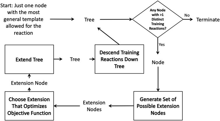
Such decision trees have been used within RMG for many years.43 However they are tedious to construct, update and maintain and their accuracy is dependent on the knowledge of the kineticists that build and maintain them. In order to automatically construct an optimal tree one could imagine searching the space of all possible decision trees. However, typically it is infeasible to do this on a given dataset due to the high dimensionality of the problem.41 It is standard instead to iterate starting from a single root node adding the new node that best optimizes the tree each iteration. The tree generation process typically ends when some termination criterion related to the number of tree nodes or tree depth is satisfied.This greedy optimization approach in our case starts to look like the diagram in Fig. 2. One starts with an initial tree (possibly only containing a single node) and a set of training reactions classified to the bottom nodes of the initial tree. We then choose any node in the tree with more than one training reaction and attempt to add new nodes that best divide those reactions into groups with similar rate estimates. This involves generating a set of possible new nodes and selecting the best extension node. After the new node is selected it is added to the tree and the training reactions are descended down to the most specific node they match. Then the iterative procedure is continued with a new node.
2.3 Generating extension nodes
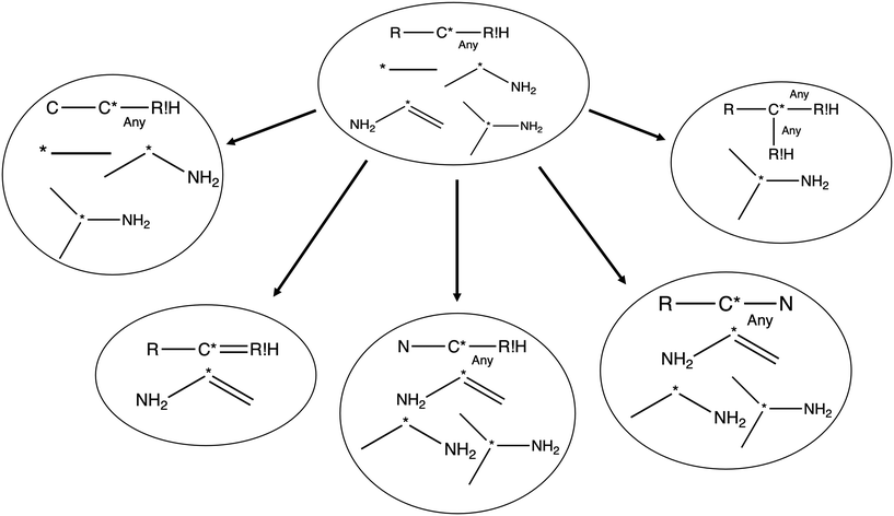
Each iteration the algorithm must generate a set of group structures subgraph-isomorphic to the structure at the chosen node. An example of extension generation is displayed in Fig. 3. The root (first) structure in the tree is user specified. Consider a simple structure: where * denotes an atom that participates in the reaction in a way that makes it unique, ? denotes a bond that has an unknown order and R denotes an unspecified atom. Most real reaction templates are more complex, but this example structure is convenient for illustrating important concepts. Structures that would match this include the following: C*H3–CH3, CH3–C*H2–NH2, NH2–C*H
![[double bond, length as m-dash]](https://www.rsc.org/images/entities/char_e001.gif) CH2, CH3–C*H(–CH3)–OH, and C*H2–CH3.
CH2, CH3–C*H(–CH3)–OH, and C*H2–CH3.
In this context it is relatively easy to start listing off ways to make atoms and bonds in  more specific. We call these specification extensions. We allow the definition of the element of an atom or the order of a bond. We also need some way to specify the presence of a radical which we add by allowing extensions to specify the number of unpaired electrons on an atom. One could also imagine situations where the charge on an atom or the number of paired electrons is important. We allow one last specification extension that specifies if an atom is in a ring or not; the significance of this will be discussed later in this paper.
To ensure we can divide arbitrary sets of reactions we need to be able to create new bonds and atoms in the structures. For this reason we define (1) an internal bond creation extension that forms bonds of undefined order between atoms present in the structure and (2) an external bond creation extension that forms a bond of undefined order between an atom in the structure and a new R!H (any atom but H).
There are a couple of nuances here. The first is that while one could define an extension that adds an unattached unspecified atom to the structure it is unlikely to provide more useful splitting than an attached unspecified atom. By extending with R!H rather than R we have made it impossible to add hydrogens to an atom in the structure. However, this only means that the way we divide reactions that have hydrogens in those locations from those that do not is by defining bonds to R!H that will only match those without hydrogens. In particular this also significantly reduces the number of extensions generated; which will be quite important later.
So far we have described individual one-step extensions we can apply to a structure, but we have not determined how we should concatenate them to generate the considered set of extensions. Naively one might consider applying extensions in N-steps where the set of one-step extensions is generated off the original structure, and then extensions off those structures and so on eventually combining them all into one set of possible extensions. However, even beyond making the number of structures combinatorically large this approach is insufficient to divide all sets of reactions.
There are a few important things to understand in these cases. First, when a selected extension is compared with the set of reactions there are three possible results: it matches none of the reactions, it matches some of the reactions or it matches all of the reactions. Second, specification extensions as defined in this study are only useful for purposes of extension selection if they match some of the reactions. Third, bond creation extensions are important when they match some or all of the reactions. Consider our structure from before  and suppose our reactions can be represented: CH3–C*H2–CH2–CH2–CH3, CH3–C*H2–CH2–OH and CH3–C*H2–CH2–CH
![[double bond, length as m-dash]](https://www.rsc.org/images/entities/char_e001.gif) O. Using one-step extensions this set of reactions cannot be divided because every one-step extension either matches all or none of the reactions. If we were to only have CH3–C*H2–CH2–CH2–CH3 and CH3–C*H2–CH2–CH
O. Using one-step extensions this set of reactions cannot be divided because every one-step extension either matches all or none of the reactions. If we were to only have CH3–C*H2–CH2–CH2–CH3 and CH3–C*H2–CH2–CH![[double bond, length as m-dash]](https://www.rsc.org/images/entities/char_e001.gif) O in fact two-step extensions would be insufficient as well. This situation is common since training reaction data are sparse. It is particularly important in reactions that involve rings.
O in fact two-step extensions would be insufficient as well. This situation is common since training reaction data are sparse. It is particularly important in reactions that involve rings.
In order to get around these issues and run efficiently we start by generating one-step extensions from the original structure. If a bond creation extension matches all of the reactions the identified tags from that iteration are applied to it and then it is treated like the original structure and first step extensions are generated for it and so on. Each specification extension that matches none of the reactions is tagged for future reference and not generated again. For example if  is found to not match any structures under
  we don't generate the atomic extensions of that particular R again when we examine
  . After this recursive procedure is run, all generated extensions that match some, but not all, of the reactions are combined to form the set of considered extensions.
Note that when we recurse on the bond creation extensions we do recheck specification extensions that matched all reactions before, even though it might seem like this would be true for all descendent structures. This is because a specification extension that matches all reactions can in some cases stop matching reactions as the structure is extended. Consider the node C*–R!H with reaction templates HO–H2C*–NH–CH3 and H2C*(–NH2)–O–CH3. Naturally the algorithm will extend C*–R!H to C*(–R!H)–R!H–R!H. However, by the time C*(–R!H)–R!H–R!H is generated the algorithm will have tagged atom extensions on the R!H atoms bonded to C* and found that both N and O match all of the reactions. If each generalization between the group and its reactions was fixed (only N or only O in the case above) it would be safe to assume a specification extension that matched all reactions would match all reactions for all subgraph isomorphic groups that matched a reaction in the set because it would be the same. However now that the third R!H is added specifying the atom type of one of the R!H atoms bonded to C* is the only way to divide the two reactions. If we were to not recheck specifying atom types for those atoms it would be impossible to divide the reaction set.
2.4 Choosing the best extension
The best extension to add to a rate tree should be the one that improves estimation the most after adding it. In an ideal situation one would fit all of the data on each side of the split to a model of choice for nodes in the tree and then run leave-one-out cross validation at a variety of temperatures to determine the differences in errors. However, our model parameters (which will be discussed later) are not analytic functions of the data, so such an analysis would be very computationally expensive.Using a variety of temperatures is also problematic. Quantum chemical rate calculations are much more accurate at higher temperatures than lower temperatures and experimental rates are often only accurate in a specific temperature range. As a result the RMG database we draw our training sets from contains many rates that aren't accurate at low or very high temperatures, however accuracy for most rates is good in the vicinity of 1000 K.
For these reasons in this work we choose extensions based on accuracy improvement at 1000 K assuming errors in the rate coefficient are lognormally distributed. We choose the extension that minimizes
| Π = N1σ1 + N2σ2 | (1) |
2.5 Extending the tree: complementary nodes
Once an extension is selected it is added to the decision tree under its parent node. If the extension does not create any bonds it is usually possible to define a complementary node that matches any reaction that matches the parent, but does not match the new node. For example if an R is defined as being a H the complement would be the same structure with R as R!H. If such a complementary node can be defined it is also added under the parent. Then reactions are descended from the parent to any of the new nodes they match.Adding complementary nodes improves readability. Suppose we have a parent node R–C*–?R!H, we select a first child node H–C*–?R!H and we do not define a complementary node. Since we still have reactions at the parent node we need to generate a second child node. For example we might generate R–C*–?R!H–?R!H a structure that isn't mutually exclusive with the other child. However, because the first child comes first in the tree no structure that matches it will be matched to the second child. This means that the R in reactions matching the second child will never be H so the second child would be more clearly written as R!H–C*–?R!H–?R!H. Adding complementary nodes when possible makes the generated tree structure easier for a human to read.
2.6 Estimating rates from the tree
Now that we have a tree we need to define precisely how we use that tree to estimate rates. We define a rule at each node. In order to do this we take all the reactions that match a given node (so the top node would have all reactions) and fit them to a Blowers–Masel interpolant.44 This interpolant developed in Blowers and Masel 2000 correlates ΔHr with Ea in a way that is much more accurate across the range of ΔHr values than other more typical forms such as Evans–Polanyi.44 The interpolant is defined by the equations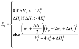 | (2) |
 | (3) |
 | (4) |
 | (5) |
 | (6) |
There are errors in ki(Tj) values, whatever their source, but some ki(T) values are very accurate. It is therefore important to assign different uncertainties ΔEij to different data. Considering the known inaccuracies in the experimental techniques several approaches have been employed to estimate uncertainties. One approach is for experts to consider all the (mostly experimental) data about individual reactions.32 Another is to further constrain ki(T) using system measurements (e.g. flame speeds).33–35 If the estimate is from theoretical calculations one can try to bound the errors due to each approximation, or more commonly compare the present reaction to other similar reactions, with known errors, computed using the same technique.37,38 RMG currently has a mix of uncertainty estimates, some very accurate but many quite rough.
If E0a < 0 the Blowers–Masel interpolant is no longer valid and we simply take averages of the parameters in our log-modified-Arrhenius expressions for each training reaction instead
 | (7) |
 | (8) |
 | (9) |
2.7 Estimating uncertainties from the tree
Estimating useful uncertainties for the input reactions, the interpolant, and particularly for the k(T) estimate for a new reaction where no data is available, is quite challenging. Most earlier attempts32–34,40 at estimating errors in rate estimates have been fairly heuristical, and many focused on not overestimating uncertainties for purposes of uncertainty analysis of full kinetic models.45,46 Here we present an automated approach focused on representing the distribution of uncertainties of each k(T) estimate.We are interested in the distribution of Δlog(ki) = log(kmodeli) − log(ktruei). For an individual training reaction rate coefficient krxni we assume that
 | (10) |
 is the variance of log(krxni) based on the uncertainty in the training reaction. We assume that the Blowers–Masel estimate of a particular reaction i, kmodeli is distributed as
 | (11) |
 is the variance associated with errors in the the Blowers–Masel parameters and kbest fiti is the output the Blowers–Masel model would give without any errors in the parameters. This hypothetical errorless Blowers–Masel is what would be achieved by fitting to an arbitrarily large number of training reactions with σrxni = 0 that match the associated node. Such an ideal model would have σmodeli, but still have error associated with the limitations of the Blowers-Masel fit form causing kbest fiti ≠ ktruei. Taking the difference between the two distributions we have
 | (12) |
 , but the other parameters are unknown and since this distribution is specific to reaction i we cannot draw samples from the node to estimate the parameters. It does, however, outline two primary sources of error in the quantity: limitations in the models ability to represent the chemical space and the errors in the training data. In general we expect there to be two limits. At lower nodes there will be fewer training reactions, but a much smaller chemical space. In this small chemical space limit we have kbest fiti ≈ ktruei and since the smaller chemical space is easier to fit with proper weighting we expect
  to be reaction independent and small giving us
 | (13) |
 | (14) |
 | (15) |
 . If high accuracy values for
  are available this is possible to do accurately. However, in this work we do not have sufficiently accurate values for
  and to ensure our estimates are reasonable we estimate all uncertainties in the other limit. This will likely cause overestimation of uncertainties at nodes that have very low uncertainties.
In the other limit at higher nodes there will be more training reactions and a larger chemical space. In this case we expect log(kbest fiti) − log(ktruei) to be large. In this case we expect the errors in kmodeli to dominate. This allows us to neglect  , although they are still necessary to use as weights. Note that when errors are properly weighted the true scale of
  is determined by the smallest value among the set of reactions. In this case however the simplification only gets us to
 | (16) |
| Δlog(ki) ∼ N(μmodel, σ2model) | (17) |
 | (18) |
 or smaller it is best to use the small chemical space approach. Although as noted above we do not have sufficiently accurate training uncertainties to accurately implement the small chemical space approach. Our implementation of the large chemical space approach is described below.
First, we estimate the distribution of errors in the training data. Training reactions within the RMG-database come from many different sources. However, the vast majority are based on quantum chemistry calculations. Rate expressions from quantum chemistry calculations primarily have four sources of error: errors in the computed frequencies, errors in the internal rotor treatment, errors in the computed energies and errors in fitting the rate coefficients to a functional form (e.g. Arrhenius equation). While the fourth is commonly reported because it is easiest to estimate it is rarely significant. The errors are most often dominated by the error in the computed energies. While one could envision complex schemes of accounting for calculation uncertainties typically only the level of theory is recorded in the RMG-database. For this reason we map RMG-database reactions' ranks (identifiers associated with source types: experiments, calculations, and estimates) to our own estimates of 2-sigma uncertainties in the Arrhenius Ea. For example a CBS-QB3 calculated rate (a typical level of theory in the RMG training data) would be associated with a 2.5 kcal mol−1 uncertainty while the least reliable data source, a “rule of thumb” generalization, would be assigned a 14 kcal mol−1 uncertainty.47 We express our errors as Δlog(k) rather than Δk because Δlog(k) ∼ ΔEa.
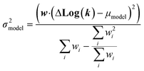
Once we have estimates of the uncertainties in the training data, we can look at estimating the uncertainties in the predictions of our new tree-based rate estimator. For similar reasons to building the tree we do this analysis at 1000 K. However, under suitable assumptions (for example all of the error being associated with Ea) it is relatively easy to reasonably extrapolate the uncertainties generated to other temperatures. For each node with more than one training reaction we compute the leave-one-out errors for the model predictions for reactions that match that node against the training reactions at 1000 K.
 | (19) |
 | (20) |
 | (21) |
 | (22) |
 | (23) |
We now have the capability to estimate reaction rate coefficients and uncertainties (based on μmodel and σ2model) at each node. This in fact provides us with many different estimates for a given k(T): one for each node in the tree a reaction matches. Naively one might think it would be best to estimate each reaction using the most specific node it matches, however, this is not always the case. At each node there is error associated with ability of the Blowers–Masel model to accurately represent all the reactions at that node, the error in the training reactions, and also error associated with the ability to accurately estimate the Blowers–Masel parameters from the available training reactions. At nodes near the top of the tree there are many reactions making it possible to accurately calculate the Blowers–Masel parameters, however, the chemical space spanned can be quite large making it difficult for a single Blowers–Masel model to represent all of the involved reactions. At nodes near the bottom of the tree the chemical space spanned is much smaller and the Blowers–Masel model can better represent the space, but there are fewer reactions to fit to making the Blowers–Masel fit sensitive to errors in the training data.
Now that we have uncertainties it is possible to use them to choose the best node to estimate from. If we think an estimate from a certain node is less accurate than estimating from its parent we can estimate from its parent instead. However, this analysis needs to balance several different kinds of error: the error expected from the model at that node, the error expected from the model at the parent node, and the error associated with using the parent node to estimate at the child node. The later may seem unimportant, but it's a very important consideration particularly in the dataset we use. This is because rate rules especially at large scale are manually constructed to generate accurate chemical kinetic models. This means that a sensitive reaction may be similar to many training reactions in the database, while an insensitive reaction may only be similar to one or two. This means we may have cases where moving up a node dramatically changes estimates. To account for these errors we add the difference in the data mean values of the distributions to the bias (model mean) of the parent distribution. Assuming errors in log(k) are distributed normally and given that for a half-normal distribution the expected value is  we can compare the expected errors. Taking an upper bound on the means gives us the criterion
 | (24) |
In the literature there are arguments that rate coefficient errors should be treated log-uniformly instead of log-normally.48 However, in practice we found when attempting to represent larger normal distributions based on small samples (2–4 data points) that treating these samples as distributed normally significantly improved agreement with the histograms over uniform when the samples were fairly representative and was roughly equally as bad as treating them uniform when they were not. However, this assumption is only made for purposes of ascending the tree during rate estimation and our uncertainty outputs are of course not distribution specific.
2.8 Regularization and embedding qualitative chemical knowledge in estimators
Fundamentally regularization is choosing between two different estimators that have similar accuracy on the data they were trained on.41 It is an important component in machine learning for avoiding overfitting or having a model that fits the training data well, but performs much more poorly on other data. In most contexts discussing the space of models with similar training accuracy is complex. However, for our subgraph isomorphic decision trees it is fairly simple.Earlier we discussed that during tree generation we tracked specification extensions in each structure down the tree that matched all of the reactions matching that node. Suppose again we have the node  and suppose our training reaction templates are CH3–C*H2–CH2–CH2–CH3, CH3–C*H2–CH2–OH and CH3–C*H2–CH2–CH
![[double bond, length as m-dash]](https://www.rsc.org/images/entities/char_e001.gif) O. It is clear here that converting R– > C for both R's in the node will not affect the training reactions that match this node and therefore not affect training errors. However, if we were to use this tree to estimate reactions represented by the templates H–C*H2–CH3 and CH3–C*H3 whether they matched the node and thus how they were estimated would be changed if one were to convert R– > C for those R's.
O. It is clear here that converting R– > C for both R's in the node will not affect the training reactions that match this node and therefore not affect training errors. However, if we were to use this tree to estimate reactions represented by the templates H–C*H2–CH3 and CH3–C*H3 whether they matched the node and thus how they were estimated would be changed if one were to convert R– > C for those R's.
Typically a model would be regularized by setting aside a test set of reactions and then tuning optimization hyperparameters according to heuristics to improve performance on the test set. This is problematic for small datasets particularly when the estimators' accuracy may depend on the presence of key reactions in the training set. Here we can simply do so by moving along these “regularization” dimensions that do not affect the training split without sacrificing any accuracy on reactions similar to the training set.
Even more beautifully these regularization dimensions are human readable. This means that we can do more than just regularize while preserving training accuracy. An expert can embed their chemical knowledge within the estimator by adjusting the regularization algorithm. Suppose we have the node  and we have training reaction templates: C*H3–CH2–CH3, C*H3–O–CH3 and C*H2
![[double bond, length as m-dash]](https://www.rsc.org/images/entities/char_e001.gif) O. A good safe default regularization choice is to make each node as specific as the reaction set that matches it so you might get post regularization C*–? [C, O]. However, suppose the expert does not think the identify of that atom is important they could choose to keep that atom general or at least extend it to another atom type. This can be particularly helpful for small datasets.
O. A good safe default regularization choice is to make each node as specific as the reaction set that matches it so you might get post regularization C*–? [C, O]. However, suppose the expert does not think the identify of that atom is important they could choose to keep that atom general or at least extend it to another atom type. This can be particularly helpful for small datasets.
The tree generation algorithm is even robust to mistakes on the part of the expert. In the last case if the identity of that atom is important you would expect the algorithm to extend the tree with C*–?O or C*–?C. The expert's choice of regularization won't affect estimation in the tree for any reaction hitting this split or below. This means that if enough data is present to learn the difference these substructures make on rate estimation any potential mistakes in the chemical knowledge embedded in the regularization will be ignored.
2.9 Performance and scaling
If our generated tree was a binary tree with perfectly even splits we would expect to have the number of nodes double until we had Nrxns nodes. The partial sum for the number of nodes in this idealized tree with k layers is 2k+1 − 1 since our last layer is 2k = Nrxns this implies that our number of nodes should be approximately 2Nrxns, which agrees well with observed tree node numbers, and scales, O(Nrxns), linearly with our number of reactions. However, the amount of work needed for each node can vary significantly, but has two primary expensive operations: making new groups which scales O(Nextensions) and identifying whether extensions map the reactions at the node which (noting that the number of reactions at a node scale with the total number of training reactions) scales O(Nnode rxnsNextensions), where Nnode rxns is the number of reactions at a node that scales linearly with Nrxns and Nextensions is the number of extensions generated at a node. This means that for large enough Nrxns the overall naive algorithm will scale quadratically with Nrxns.In practice the algorithm works quite efficiently serially on datasets that tend to have low numbers of heavy atoms or are small. For these datasets training times using the naive algorithm are at most an hour. This heavy atom dependence comes from its impact on Nextensions. Larger numbers of heavy atoms make it possible to have nodes where all the reactions involve large species that are nearly identical around the reactive sites. In these extension generation cases Nextensions can combinatorically explode from repeatedly generating bond extensions that need to be extended themselves resulting in Nextensions being several orders of magnitude larger than is typical. This becomes problematic for a couple of RMG families that contain 3000–6000 reactions a significant subset of which have many heavy atoms.
Fitting the Blower–Masel interpolants could also be limiting in the overall process of generating an estimator. Fitting an interpolant scales roughly O(Nrxns) so naively running the fitting at every node will scale roughly quadratically. However, one can set a maximum number of reactions Nmax and using stratified sampling based on rate values at a chosen temperature to select a representative subset of Nmax reactions to fit to. Fitting on this subset of reactions is O(1) making the overall fitting process scale linearly with the number of reactions. However, we have not found this process to be limiting in practice so this approach is not implemented here.
We have developed techniques that enable parallelization of tree generation, avoid computational explosion in extension generation and enable linear scaling with respect to Nrxns.
The construction of subtrees that don't intersect with each other is embarrassingly parallel, but are dependent on the shared nodes above. The parallelization is handled recursively. Processes have an assigned subtree and a specific number of processors at their disposal. If a split divides the set of reactions into large enough chunks that it is worth sending information to another processor it will generate a subprocess that is assigned an associated subtree in the split and an appropriate number of processors for the size of that subtree. When a process completes its subtree it sends the subtree back to the process that spawned it and so on until the entire tree is constructed.
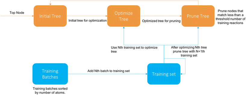
The cascade algorithm operates on the principle that we feed data to the training algorithm as needed to extend the tree properly instead of all at once. A diagram of the algorithm is available in Fig. 4.
We first sort the reactions based on their number of atoms and divide them into batches of a specified size. The first iteration the tree is trained on the first batch like normal. After the Nth tree generation the N + 1th batch (if it exists) is added and descends down the tree. Then the tree is pruned, removing all nodes that have more than a set fraction of reactions from the latest batch, and then reoptimized with the new reactions. Once there are no batches left it terminates after optimization.
Normally if a bond formation extension matches all reactions the resulting structure is sent to be extended itself. This ensures that every set of reactions can be split. However it is very expensive because computing extensions for each new structure is roughly as expensive as the original extension generation step and the number of extensions has a tendency to combinatorically explode. Even worse, unless these extensions are linking back to another reaction site or forming a ring they typically won't have much of an affect on the reaction rate. This means they won't be picked and will likely end up regenerated entirely when extensions are generated a level down the tree.
We added the ability to cap the recursion depth for extension generation as long as a splitting extension has already been found. Tests capping the depth at one recursion on intra-molecular hydrogen transfer actually showed a small, but measurable decrease in error (except for median error that increased by only a factor 1.04) suggesting this has relatively minimal impact on accuracy.
We also added the ability to end splitting attempts if the recursion is returning more than a set number of extensions. This robustly prevents combinatoric explosion. One can certainly contrive counter examples where this choice might be problematic. However, in practice with a cap of 100 extensions this has only been observed to affect nodes with only two reactions present.
3 Results and discussion
3.1 Rate estimation
Estimators were generated using the training sets for RMG's oxygen substitution, intra-molecular hydrogen transfer, internal endocyclic radical addition, radical addition and hydrogen abstraction families. These reaction families were chosen primarily because they have larger training sets and higher variances in their rate coefficients. On Github, the associated database state is available on the sidt_paper branch of the RMG-database and the associated code state used is available on the sidt_paper branch of RMG-Py. All of these except internal endocyclic radical addition and radical addition are their own reverse and the reversed reactions were used as a part of the training set. Note that we count these reversed reactions when giving the number of reactions in the training set. The templates for these reactions are available in Table 2.All RMG families tested except for hydrogen abstraction and radical addition were trained on the vanilla algorithm capping the number of recursions at two and capping the number of recursion items at 100 in less than two hours. Hydrogen abstraction and radical addition were both trained in less than 7 hours using the cascade algorithm with a batch size of 1000, a reoptimization fraction of 0.25 and fitting the interpolants in parallel on six cores. The default regularization scheme was used for all families.
Reaction family error factors based on leave-one-out cross validation are available in Table 1. Histograms of leave-one-out errors are available in Fig. 5–8. The subgraph isomorphic decision tree (SIDT) estimator is a significant improvement over RMG's RR scheme in every category for every reaction family and in a number of cases approaches the dataset error limits. We can see both significant improvements in the estimation of reactions RR already predicts well and very large improvements in the estimation of reactions not predicted well by RR. Differences in prediction performance on different reaction families are best understood as result of different overall variances in the rate coefficient values, different quantities of training reactions, different training reaction accuracies and different overall chemical scopes.
| Estimator | O-Sub RR | O-Sub SIDT | Intra-H RR | Intra-H SIDT | Int-Endo RR | Int-Endo SIDT | R-Add RR | R-Add SIDT | H-Abs RR | H-Abs SIDT |
|---|---|---|---|---|---|---|---|---|---|---|
| Median absolute error factor | 10.3 | 5.28 | 8.94 | 3.56 | 9.67 | 1.73 | 2.25 | 1.88 | 5.11 | 4.05 |
| MAE factor | 18.5 | 10.1 | 38.1 | 10.9 | 24.7 | 2.95 | 3.07 | 2.34 | 16.4 | 8.02 |
| RMSE factor | 61.7 | 27.6 | 575 | 79.3 | 98.3 | 7.07 | 5.59 | 3.51 | 89.7 | 23.7 |
| 2-Sigma error factor | 3876 | 770 | 333![[thin space (1/6-em)]](https://www.rsc.org/images/entities/char_2009.gif) 000 000 |
6320 | 9710 | 50.1 | 31.3 | 12.3 | 8040 | 564 |
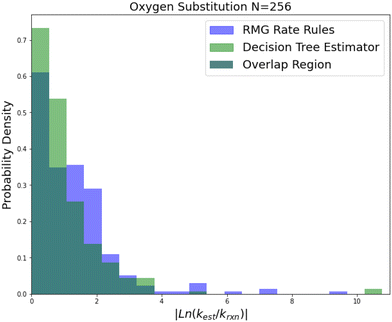 | ||
| Fig. 5 Histogram of errors for oxygen substitution reactions. Dark green is overlap. Trained on 256 reactions. | ||
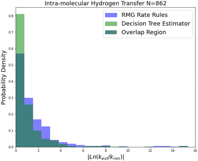 | ||
| Fig. 6 Histogram of errors for intra-molecular hydrogen transfer reactions. Dark green is overlap. Trained on 422 reactions. | ||
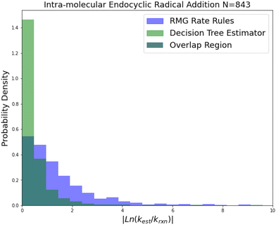 | ||
| Fig. 7 Histogram of errors for intramolecular endocyclic radical addition reactions. Dark green is overlap. Trained on 843 reactions. | ||
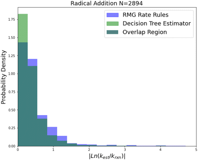 | ||
| Fig. 8 Histogram of errors for radical addition reactions. Dark green is overlap. Trained on 2892 reactions. | ||
Oxygen substitution is a particularly useful test case because the training set is entirely CBS-QB3 calculations. In this case the improvement is pretty consistent: about a factor of 2–5 in all errors. Given that the median absolute error achieved by SIDT is 5.28, which corresponds to roughly 3.34 kcal mol−1 in terms of energy, and the training set assuming a lognormal distribution only has a median absolute error of about 0.84 kcal mol−1 this set provides a good idea of performance improvement away from the training set limit. It also shows the performance of this method on small training sets.
Intra-molecular hydrogen transfer is a reaction family of more practical interest than oxygen substitution. The training set is mostly CBS-QB3 calculations, but integrates some DFT calculations and literature estimates. The accuracy improvements mostly decrease for this family across 2-sigma errors, RMSE errors, MAE errors to median absolute errors implying that the accuracy improvements on reactions not predicted well by RR are much larger than those for reactions that are predicted well by RR.
Internal endocyclic radical addition is another important reaction family and is one of RMG's larger families with 843 reactions. The training reactions are mostly CBS-QB3 calculations, with a handful of G3 calculations and literature estimates. An enormous improvement in estimation for this family is visible in Fig. 7. The 2-sigma improvement is larger than the other improvements this time as well (∼190×), but the improvement is more consistent across the other metrics. Impressively the median absolute error for this family in terms of energy corresponds to 1.09 kcal mol−1 while the training set median absolute error assumed all CBS-QB3 calculations should be about 0.84 kcal mol−1. This amounts to about a 10% error against the training set at 1000 K. This suggests that there is little room for improvement over the SIDT estimator on the best-estimated 50% of reactions in this family.
Radical addition is an important reaction family and this is reflected in the size of its 2892 reaction training set. This training set however is mostly estimates based on a reaction group additivity scheme, except for about 400 reactions that are mostly calculations at the CBS-QB3 level of theory or better. However, it is clear that these estimates must at least have low uncorrelated errors because once again we can see that SIDT is achieving a median accuracy of 1.25 kcal mol−1 not much larger than the 0.88 kcal mol−1 limit of a pure CBS-QB3 dataset. The associated histograms are available in Fig. 8. While the improvements for this family are smaller this seems likely to be a result of the fact that the accuracy of this family is being limited by the quality of the training data.
Hydrogen abstraction is another important reaction family. Much like radical addition the training set is mostly estimates from a group additivity scheme along with CBS-QB3 or better calculations and some estimates. The comparison histogram is available in Fig. 9. The improvements are more similar to those in intra-molecular hydrogen transfer being greatest for 2-sigma error and gradually decreasing across RMSE error, MAE error and median absolute error. However, in general the lower median accuracy for both RR and SIDT and the low improvement in median accuracy relative to the other smaller families suggests that either the training set is less accurate or the estimation problem is simply more difficult for hydrogen abstraction.
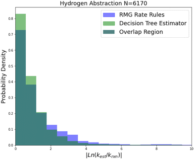 | ||
| Fig. 9 Histogram of errors for bimolecular hydrogen abstraction reactions. Dark green is overlap. Trained on 6170 reactions. | ||
3.2 Uncertainty estimation
Examining the accuracy of uncertainties is significantly more difficult than that of predictions. A histogram of errors in log(k(1000 K)) normalized by their uncertainty distribution parameters is available in Fig. 10. The SIDT uncertainty estimates approach the ideal standard normal distribution much closer than the heuristical uncertainties from Gao et al. 2020.45 Here the SIDT is able to achieve a mean and standard deviation of 0.09 and 1.21 respectively compared to −0.172 and 3.30 from the heuristics.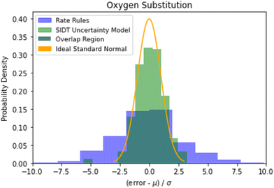 | ||
| Fig. 10 Histogram of normalized errors for the oxygen substitution reactions. The uncertainties in rate rules (purple) are taken from Gao et al. 2020.45 Ideally at high sample sizes the histogram should become a normal distribution. | ||
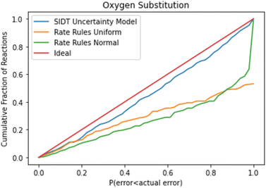
A cumulative histogram of the probability of errors is available in Fig. 11. This plot is a bit more difficult to interpret. Uncertainty models above the red “ideal” line are overpredicting the uncertainties while those under the line are underpredicting uncertainties. Along the x-axis the histogram is excluding reactions with larger and larger errors normalized by their predicted uncertainty. From this plot we can conclude that while all methods underpredict uncertainties in this family the SIDT uncertainty model underpredicts by significantly less than the heuristics from Gao et al. 2020.45
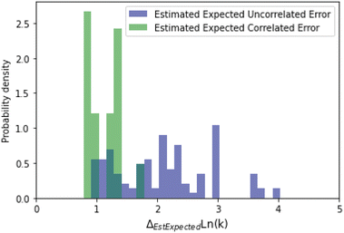
A histogram of the expected correlated and uncorrelated errors for oxygen substitution reactions is shown in Fig. 12. As one might expect for a tree-based estimator, some of the errors are correlated and some uncorrelated.
The normalized error results for SIDT for the other reaction classes are available in Table 3 and Fig. 13. All of the reaction classes have normalized standard deviations under 1.5, however, the larger families (radical addition and hydrogen abstraction) achieve values much closer to 1.0. The cumulative histograms for SIDT for the other reaction classes are available in Fig. 14. While the error estimates for intra-molecular hydrogen transfer and bimolecular hydrogen abstraction reactions are close to ideal the SIDT often underestimates the true uncertainties for bimolecular radical addition and intramolecular endocyclic radical addition reactions.
| Reaction class | O-Sub | Intra-H | Int-Endo | R-Add | H-Abs | Ideal |
|---|---|---|---|---|---|---|
| Mean | 0.09 | 0.14 | −0.08 | 0.21 | 0.03 | 0.0 |
| Std | 1.21 | 1.48 | 1.47 | 1.04 | 1.19 | 1.0 |
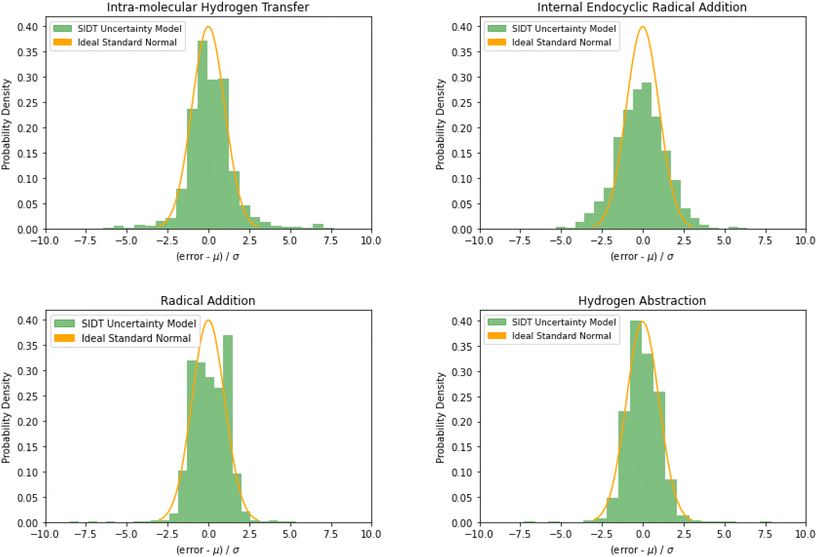 | ||
| Fig. 13 Histograms of normalized errors. Ideally at high sample sizes the histogram should match the standard normal density function. | ||
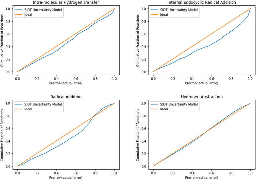 | ||
| Fig. 14 Cumulative histogram of the probability that the uncertainty estimate from SIDT is less than the actual leave-one-out error. | ||
4 Conclusions
We have presented a machine learning based estimator automatically trainable from an arbitrary set of reactions. This estimator is highly scalable from very small to large dataset sizes and is easy to update. In spite of the use of machine learning the estimator is equally human readable and human manipulable as the RR scheme it is compared against. It can naturally embed qualitative chemical knowledge from experts to improve estimation. Additionally, it incorporates accurate uncertainty estimation and provides properties of the uncertainty distribution that enable the information to be used in many contexts. The SIDT estimator has demonstrated significant accuracy improvements over the state of the art in most cases and measures and has been demonstrated to approach the accuracy limits of the dataset in some cases.While the presented technique learns reaction rates that occur as a function of specific sites on a molecule, the SIDT approach is relatively easy to extend to whole molecule properties. One simply needs to define an appropriate summation scheme and interpolant, a new objective function, and a technique for picking which nodes to extend first (as unlike in the current scheme the order in which nodes are extended may matter). The remaining machinery remains the same.
As we look forward to the future of kinetics and other property estimators it is important to keep in mind the needs of mechanism builders and the kinetics community as a whole. Having high accuracy today is convenient, but even more important is the ability to easily improve and extend the estimator in the future. The method presented here provides the user with uncertainty estimates to help determine what can be and needs to be improved, human readability to determine how to improve the estimator, and scalability and automatic training to easily update the estimator. We hope to provide a new standard for what mechanism builders should expect from their property estimators.
Conflicts of interest
There are no conflicts to declare.Acknowledgements
This material is based upon work supported by the U.S. Department of Energy's Office of Energy Efficiency and Renewable Energy (EERE) under Award Number DE-EE0007982 (Co-Optima). This research was supported by the Exascale Computing Project (ECP), Project Number: 17-SC-20-SC, a collaborative effort of two DOE organizations, the Office of Science and the National Nuclear Security Administration, responsible for the planning and preparation of a capable exascale ecosystem including software, applications, hardware, advanced system engineering, and early test bed platforms to support the nation's exascale computing imperative.Disclaimer: this report was prepared as an account of work sponsored by an agency of the United States Government. Neither the United States Government nor any agency thereof, nor any of their employees, makes any warranty, express or implied, or assumes any legal liability or responsibility for the accuracy, completeness, or usefulness of any information, apparatus, product, or process disclosed, or represents that its use would not infringe privately owned rights. Reference herein to any specific commercial product, process, or service by trade name, trademark, manufacturer, or otherwise does not necessarily constitute or imply its endorsement, recommendation, or favoring by the United States Government or any agency thereof. The views and opinions of authors expressed herein do not necessarily state or reflect those of the United States Government or any agency thereof.
Notes and references
- M. S. Johnson, M. R. Nimlos, E. Ninnemann, A. Laich, G. M. Fioroni, D. Kang, L. Bu, D. Ranasinghe, S. Khanniche, S. S. Goldsborough, S. S. Vasu and W. H. Green, Int. J. Chem. Kinet., 2021, 53, 915–938 CrossRef CAS.
- M. Liu, A. G. Dana, M. S. Johnson, M. J. Goldman, A. Jocher, A. M. Payne, C. A. Grambow, K. Han, N. W. Yee, E. J. Mazeau, K. Blondal, R. H. West, C. F. Goldsmith and W. H. Green, J. Chem. Inf. Model., 2021, 61, 2686–2696 CrossRef CAS PubMed.
- M. S. Johnson, X. Dong, A. G. Dana, Y. Chung, J. D. Farina, R. J. Gillis, M. Liu, N. W. Yee, K. Blondal, E. Mazeau, C. A. Grambow, A. M. Payne, K. A. Spiekermann, H.-W. Pang, C. F. Goldsmith, R. H. West and W. H. Green, J. Chem. Inf. Model., 2022, 62, 4906–4915 CrossRef CAS PubMed.
- C. W. Gao, J. W. Allen, W. H. Green and R. H. West, Comput. Phys. Commun., 2016, 203, 212–225 CrossRef CAS.
- R. G. Susnow, A. M. Dean, W. H. Green, P. Peczak and L. J. Broadbelt, J. Phys. Chem. A, 1997, 101, 3731–3740 CrossRef CAS.
- J. Zador and J. A. Miller, Proc. Combust. Inst., 2015, 35, 181–188 CrossRef CAS.
- P. L. Bhoorasingh, B. L. Slakman, F. Seyedzadeh Khanshan, J. Y. Cain and R. H. West, J. Phys. Chem. A, 2017, 121, 6896–6904 CrossRef CAS PubMed.
- G. Henkelman, B. P. Uberuaga and H. Jonsson, J. Chem. Phys., 2000, 113, 9901–9904 CrossRef CAS.
- M. S. Johnson, M. Gierada, E. D. Hermes, D. H. Bross, K. Sargsyan, H. N. Najm and J. Zador, J. Chem. Inf. Model., 2023, 63, 5168 CrossRef PubMed.
- P. Zimmerman, J. Chem. Theory Comput., 2013, 9, 3043–3050 CrossRef CAS PubMed.
- S. Maeda, T. Taketsugu and K. Morokuma, J. Comput. Chem., 2014, 35, 166–173 CrossRef CAS PubMed.
- Y. V. Suleimanov and W. H. Green, J. Chem. Theory Comput., 2015, 11, 4248–4259 CrossRef CAS PubMed.
- A. G. Dana, D. Ranasinghe, O. H. Wu, C. Grambow, X. Dong, M. S. Johnson, M. Goldman, M. Liu and W. H. Green, ARC – Automated Rate Calculator, https://github.com/ReactionMechanismGenerator/ARC Search PubMed.
- S. N. Elliott, K. B. Moore, A. V. Copan, M. Keceli, C. Cavallotti, Y. Georgievskii, H. F. Schaefer and S. J. Klippenstein, Proc. Combust. Inst., 2021, 38, 375–384 CrossRef CAS.
- C. A. Grambow, A. Jamal, Y.-P. Li, W. H. Green, J. Zador and Y. V. Suleimanov, J. Am. Chem. Soc., 2018, 140, 1035–1048 CrossRef CAS PubMed.
- S. Maeda and Y. Harabuchi, J. Chem. Theory Comput., 2019, 15, 2111–2115 CrossRef CAS PubMed.
- C. A. Grambow, L. Pattanaik and W. H. Green, J. Phys. Chem. Lett., 2020, 11, 2992–2997 CrossRef CAS PubMed.
- K. Spiekermann, L. Pattanaik and W. H. Green, Sci. Data, 2022, 9, 1–12 CrossRef PubMed.
- L. Pattanaik, PhD thesis, Massachusetts Institute of Technology, 2023 Search PubMed.
- K. A. Spiekermann, L. Pattanaik and W. H. Green, J. Phys. Chem. A, 2022, 126, 3976–3986 CrossRef CAS PubMed.
- O.-E. Ganea, C. W. Coley, R. Barzilay, K. F. Jensen, W. H. Green and T. S. Jaakkola, Advances in Neural Information Processing Systems, 2021, vol. 34, pp. 13757–13769 Search PubMed.
- E. Heid and W. H. Green, J. Chem. Inf. Model., 2022, 62, 2101–2110 CrossRef CAS PubMed.
- S. W. Benson and J. H. Buss, J. Chem. Phys., 1958, 29, 546–572 CrossRef CAS.
- R. Van de Vijver, M. K. Sabbe, M.-F. Reyniers, K. M. Van Geem and G. B. Marin, Phys. Chem. Chem. Phys., 2018, 20, 10877–10894 RSC.
- H. H. Carstensen and A. M. Dean, J. Phys. Chem. A, 2009, 113, 367–380 CrossRef CAS PubMed.
- R. Sumathi and W. H. Green, J. Phys. Chem. A, 2002, 106, 5474–5489 CrossRef CAS.
- R. H. West, J. W. Allen and W. H. Green, ChemInform, 2012, 43(36) DOI:10.1002/chin.201236258.
- M. Saeys, M.-F. Reyniers, V. Van Speybroeck, M. Waroquier and G. B. Marin, ChemPhysChem, 2006, 7, 188–199 CrossRef CAS PubMed.
- J. W. Allen, PhD thesis, Massachusetts Institute of Technology, 2013 Search PubMed.
- S. Choi, Y. Kim, J. W. Kim, Z. Kim and W. Y. Kim, Chem. – Eur. J., 2018, 24, 12354–12358 CrossRef CAS PubMed.
- S. Datta, V. A. Dev and M. R. Eden, Comput. Chem. Eng., 2017, 106, 690–698 CrossRef CAS.
- D. L. Baulch, M. J. Pilling, C. J. Cobos, R. A. Cox, C. Esser, P. Frank, T. Just, J. A. Kerr, J. Troe, R. W. Walker and J. Warnatz, J. Phys. Chem. Ref. Data, 1992, 21, 411–734 CrossRef CAS.
- M. Frenklach, A. Packard and P. Seiler, Proc. Am. Control Conf., 2002, 4135–4140 Search PubMed.
- D. A. Sheen, X. You, H. Wang and T. Løvås, Proc. Combust. Inst., 2009, 32I, 535–542 CrossRef.
- H. Wang and D. A. Sheen, Prog. Energy Combust. Sci., 2015, 47, 1–31 CrossRef.
- N. Galagali and Y. M. Marzouk, Chem. Eng. Sci., 2015, 123, 170–190 CrossRef CAS.
- C. F. Goldsmith, A. S. Tomlin and S. J. Klippenstein, Proc. Combust. Inst., 2013, 34, 177–185 CrossRef CAS.
- L. Xing, S. Li, Z. Wang, B. Yang, S. J. Klippenstein and F. Zhang, Combust. Flame, 2015, 162, 3427–3436 CrossRef CAS.
- L. Lei and M. P. Burke, Combust. Flame, 2020, 213, 467–474 CrossRef CAS.
- T. Nagy and T. Turanyi, Int. J. Chem. Kinet., 2011, 43, 359–378 CrossRef CAS.
- C. M. Bishop, Pattern Recognition and Machine Learning, 2006, pp. 1–711 Search PubMed.
- A. Varnek, D. Fourches, F. Hoonakker and V. P. Solov'ev, J. Comput.-Aided Mol. Des., 2005, 19, 693–703 CrossRef CAS PubMed.
- W. H. Green, Adv. Chem. Eng., 2007, 32, 1–50 CAS.
- P. Blowers and R. Masel, AIChE J., 2000, 46, 2041–2052 CrossRef CAS.
- C. W. Gao, M. Liu and W. H. Green, Int. J. Chem. Kinet., 2020, 52, 266–282 CrossRef CAS.
- A. Fridlyand, M. S. Johnson, S. S. Goldsborough, R. H. West, M. J. McNenly, M. Mehl and W. J. Pitz, Combust. Flame, 2017, 180, 239–249 CrossRef CAS.
- K. P. Somers and J. M. Simmie, J. Phys. Chem. A, 2015, 119, 8922–8933 CrossRef CAS PubMed.
- T. Nagy, E. Valko, I. Sedyo, I. G. Zsely, M. J. Pilling and T. Turanyi, Combust. Flame, 2015, 162, 2059–2076 CrossRef CAS.
Footnote |
| † Electronic supplementary information (ESI) available: The software and datasets used here are available on GitHub in the RMG-Py and RMG-database repositories. A Jupyter notebook is available in the RMG-database repository for generating and fitting kinetics trees as done in this work. The specific code and database states used in this work are available on the sidt_paper branches of these repositories. The supporting information contains error histograms for radical recombination, disproportionation and keto-enol reaction families. See DOI: https://doi.org/10.1039/d3re00684k |
| This journal is © The Royal Society of Chemistry 2024 |

