Machine learning for revealing the relationship between the process–structure–properties of polypropylene in-reactor alloys

Abstract

Polypropylene in-reactor alloys present a complex structure influenced by diverse polymerization process parameters, posing challenges for traditional analysis methods in establishing a quantitative relationship between process conditions, alloy structures and mechanical properties. To address this issue, a series of polypropylene/poly(ethylene-co-propylene) alloys with varied structures were synthesized by gas-phase polymerization. Machine learning methods were employed to develop regression models for predicting flexural strength (FS), impact strength (IS) and rubber phase content. The importance of structure and process condition descriptors was further analysed to reveal the process–structure–property relationship. The FS and IS prediction models utilizing Extreme Gradient Boosting (XGB) algorithms achieved impressive R² scores of 0.9846 and 0.9841, respectively. Notably, the significant contribution of the rubber phase content to FS and IS prediction was observed in the structure descriptors. Furthermore, process condition descriptors (flowrate and initial pressure) played crucial roles in rubber synthesis, thereby exerting a substantial impact on FS and IS. In light of the feature importance analysis, new experimental runs were designed to synthesize alloys with enhanced IS. The experimental results closely aligned with the model predictions (RMSE = 4.4751 for IS). This research provides a new approach to establish process–structure–property relationships for in-reactor alloys, providing a convenient method for designing experiments to attain desired material properties.

---

1. Introduction

The use of polypropylene (PP) in-reactor alloys is an effective approach^1–3 to significantly improve the typically low impact strength⁴ of polypropylene. This technique involves the homo-polymerization of propylene to produce PP, followed by copolymerization of propylene and ethylene, resulting in the formation of a copolymer (ethylene–propylene rubber).⁵ This approach circumvents the challenges associated with achieving effective mixing on submicron scales between the rubber phase and PP phase using traditional mixing processes.⁶ However, this advancement introduces new complexities as the structure of the in-reactor alloy becomes more complicated⁷ due to copolymerization reactions, yielding products such as block copolymers and random copolymers.⁸ Additionally, controlling the composition, melt index, crystallinity, and other structural characteristics of the alloys becomes a more intricate task. Analysing the complex relationships between the structure and properties, as well as the interplay between process conditions and the structure in polypropylene alloys, presents additional challenges.^9,10 Traditional analytical methods struggle to provide quantitative insights into these multidimensional problems. In response to these challenges, machine learning methods have been employed to predict the performance of polymer alloys and composites.^11–13

Machine learning methods excel at discovering the relationships among data points, making them valuable tools for handling nonlinear and multidimensional data.¹⁴ Consequently, machine learning has been widely used in structure determination, performance prediction and new material discovery.^15,16 Bhowmik et al. employed Decision Tree and principal component analysis methods to successfully predict the specific heat capacity of polymers using various structural descriptors, including bonds, angles, atoms and molecular weights.¹⁷ Joo et al. developed prediction models for the physical properties of polypropylene composites, employing three machine learning methods: multiple linear regression, deep neural network and Random Forest. The study analysed the impact of components in the composite materials on model predictions, providing insights for developing new recipes to achieve specific physical properties in PP composites.^18,19

Due to the prolonged polymerization time and characterization periods, the application of machine learning in polymer science and engineering has been limited, especially in smaller datasets.²⁰ Nevertheless, certain machine learning algorithms continue to demonstrate good performance even with relatively small datasets. Cai et al. applied six machine learning techniques to model the relationship between the dynamic strength of 3D-printed PP-based composites and the associated materials and printing parameters.²¹ Despite having only 26 data points, the artificial neural network achieved the highest prediction accuracy, albeit with a trade-off in computational efficiency. Kamireddi et al. performed 13 microwave-assisted catalytic co-pyrolysis experiments of PP and polystyrene (PS) mixtures and used machine learning to estimate the impact of the PP and PS quantity on the oil yield, gas yield and pyrolysis time.²² Wu et al. conducted injection molding of isotactic polypropylene into 27 specimens, collecting data on the polymorphic structure and mechanical properties to develop four machine learning models.²³ The XGB model has the highest prediction accuracy for polymorphic form contents and mechanical properties based on the various processing parameters. Their analysis highlighted that the injection pressure and shear rate charged a higher contribution to the polymorphic form, while the molding temperature played a crucial role in property prediction. Liu et al. conducted 30 polyoxymethylene gear durability tests and developed a machine learning model to assess fatigue reliability. This research offered valuable insights into the evaluation of polymer gear reliability under a limited dataset.²⁴

Some studies employed algorithms to augment the original small raw dataset before modelling.²⁵ Li et al. employed the nearest neighbour interpolation algorithm to expand a small dataset of only 23 data points and then established an XGB model to predict Akron abrasion of rubber.²⁶ Through the analysis of feature importance, the Akron abrasion was found to be most strongly correlated with the elongation at break of polymer materials. In addition, Shen and Qian proposed a virtual sample generation method to create models for predicting the wear resistance of rubber materials.²⁷ They expanded the training dataset, originally containing only 24 rubber composite samples, using a Gaussian mixture model. The results show that the algorithms can achieve high prediction accuracy even with a small sample size.

In this work, a series of polypropylene/poly(ethylene-co-propylene) in-reactor alloys were synthesized through homo-polymerization of propylene and copolymerization of propylene and ethylene. The alloy structure was systematically varied by adjusting the process conditions during the gas-phase copolymerization stage. Three machine learning algorithms, namely Decision Tree (DT), Random Forest (RF) and Extreme Gradient Boosting (XGB), were used to develop regression models for predicting mechanical properties based on the structural characteristics of the polymer alloy. The model with the best performance was further utilized to uncover the relationship between the process conditions and structure. The importance of structure and process condition descriptors was analysed. In light of the feature importance analysis, new experimental runs were designed to validate the model's accuracy.

2. Experiment and modelling

2.1. Polymerization procedure and device

The experimental device and procedure are illustrated in Fig. 1. The polymerization process was divided into three stages: propylene prepolymerization, homopolymerization and ethylene–propylene copolymerization. The primary catalyst employed was the MgCl₂-supported Ziegler–Natta catalyst, with triethylaluminum as the cocatalyst and cyclohexyldimethoxymethylsilane as the donor. In the initial stage, the catalyst, cocatalyst, donor, propylene and hydrogen were introduced to a 12 L reactor (Reactor1) for propylene prepolymerization and homopolymerization. The pre-polymerization temperature was carried out at 25 °C for 0.5 h, followed by homopolymerization at 70 °C for 1 h. Subsequently, the resulting polypropylene particles were transferred to a 25 L reactor (Reactor2). In Reactor2, a continuous feed of a mixture of ethylene, propylene and hydrogen in a specific proportion was maintained for the copolymerization of ethylene and propylene, with the temperature set at 75 °C.

Fig. 1 Flow chart of the experimental device and polymerization procedures.

The process conditions for the prepolymerization and homopolymerization stages were kept constant, while the process conditions for the gas-phase reaction were varied. These variations included changes in the ratio of ethylene (C2 in), propylene (C3 in), and hydrogen (H2 in) in the feed, as well as the flowrate of the mixture gas feed, the initial gas-phase copolymerization pressure (initial P), and the copolymerization duration (time). This variation allowed for the preparation of a series of polypropylene/ethylene–propylene copolymer alloys with different structures. The specific process conditions of gas phase polymerization are listed in Table 1 (for all datapoints, refer to ESI† Table S1). It's worth noting that “initial P” refers to the pressure in the reactor after the transfer of polypropylene particles to Reactor2, followed by the introduction of ethylene to raise the gas-phase reaction pressure to 1.4 MPa.

Table 1 The process conditions of gas-phase copolymerization

Entry	C2 in	C3 in	H2 in	Initial P (MPa)	Flowrate (kg h^−1)	Time (min)
Run 1	0.403	0.597	0.000	0.84	1.86	75
Run 2	0.397	0.596	0.007	1.12	2.52	45
Run 3	0.392	0.593	0.015	1.12	2.79	75
Run26	0.391	0.598	0.011	1.12	3.17	75
Run27	0.445	0.550	0.005	1.03	2.35	75

---

2.2. Polymer characterization

An extractive fractionation process was conducted on the alloys using n-octane and n-heptane as solvents. Each polymer alloy was separated into three fractions: F1, soluble in n-octane at room temperature; F2, soluble in boiling n-heptane; F3, insoluble in boiling n-heptane. The three fractions F1, F2, and F3 correspond to ethylene–propylene random copolymer, ethylene–propylene segmented copolymer, and isotactic polypropylene.^28,29 The two copolymer fractions soluble in the solvent constitute the rubber phase, which is dispersed within the matrix phase of isotactic polypropylene.

The crystallinity of polymer particles (Xc) was assessed via differential scanning calorimetry. Nuclear magnetic resonance and Fourier-transform infrared spectroscopy were employed to determine the content of ethylene units in the polymer chain. Additionally, the melt index (MI) of the polymer particles was measured using a melt flow indexer according to ISO 1133-1:2011. Polymer granules underwent extrusion and injection molding processes to yield specimens suitable for impact and flexural testing. The flexural strength (FS) of specimens was tested using a universal material testing machine according to ISO 178:2001, while the impact strength (IS) at room temperature was assessed using a pendulum impact tester according to ISO 180:2000.

The characterization data of the polymer alloy are shown in Table 2 (for all datapoints, refer to ESI† Table S2).

Table 2 Structure and mechanical properties of polymer alloys

Entry	Rubber (wt%)	MI (wt%)	Ethylene (wt%)	F1 (wt%)	F2 (wt%)	F3 (wt%)	Xc (%)	FS (MPa)	IS (kJ m^−2)
Run 1	16.23	11.97	29.87	12.07	4.16	83.77	43.97	22.40	10.81
Run 2	31.75	8.04	22.76	26.57	5.18	68.25	36.85	16.49	45.37
Run 3	43.98	25.92	28.75	34.93	9.05	56.02	29.84	11.61	36.83
Run 26	39.13	8.55	26.75	30.40	8.73	60.87	33.42	13.88	46.55
Run 27	34.50	6.20	23.09	22.23	12.27	65.50	36.08	14.92	55.87

---

2.3. Modelling with machine learning techniques

To determine the most appropriate models for predicting the mechanical properties of polypropylene alloys and revealing the relationship between the structure and properties, three commonly employed machine learning algorithms for regression tasks were applied, namely Decision Tree,³⁰ Random Forest,³¹ and Extreme Gradient Boosting.³² The dataset used for machine learning modelling was constructed based on the polymer characterization results (seen in Table S2†). The dataset was split in the ratio of 8 : 2 into training and testing sets. Input features included the MI, Xc, the content of rubber phase and ethylene, F1, F2, and F3, while mechanical properties FS and IS served as the output variables.

The coefficient of determination (R²) and the root mean square error (RMSE) were used as the evaluation metrics for assessing regression models. These evaluation criteria are calculated as the following equations.

where y_i, y̅, and y′_i represent the actual value, mean value and predicted value, respectively. The variable i is the index value, and n denotes the total number of samples.

Through comparative analysis, the most optimal model among these three was identified. In addition, an in-depth investigation into the interrelationship between the structure and properties of polypropylene alloys was conducted. Furthermore, employing the most suitable algorithm, machine learning models were developed to elucidate the correlations between process conditions and structural characteristics, as well as process conditions and mechanical properties. In this phase of research, the dataset was created using the process conditions (seen in Table S1†), polymer structure and mechanical properties. Input features included C2 in, C3 in, H2 in, initial P and time, while the rubber phase content or mechanical properties FS and IS were taken as the output variables.

After optimizing the hyperparameters, both the training and testing datasets were employed to assess the model's fitting performance and generalization capability. Additionally, the SHapley Additive exPlanations (SHAP) technique was applied to explicate the output of machine learning models, providing insights into the importance of individual input features in predicting a specific model outcome.^33–35

3. Results and discussion

3.1. Performance evaluation of three models

The results of the DT, RF and XGB prediction models for flexural and impact strength are illustrated in Fig. 2. The dots represent the models' predictions on the training and testing data, while the solid black line represents perfect agreement between predicted and actual values. A small distance between the dots and the line signifies excellent model prediction. As shown in Fig. 2, all three models demonstrate reasonably good performance, with data points closely aligned with the line. Among them, XGB presents in general the best performance.

Fig. 2 Parity plots of DT, RF, and XGB models using structural characteristics to predict mechanical properties; the reference line (y = x) represents perfect prediction alignment between actual and predicted values.

Fig. 3 presents the R² score of the three models on the training and testing data. It is obvious that the DT model presents typical overfitting, characterized by a lower R² score for the testing set compared to the training set, particularly when predicting flexural strength.

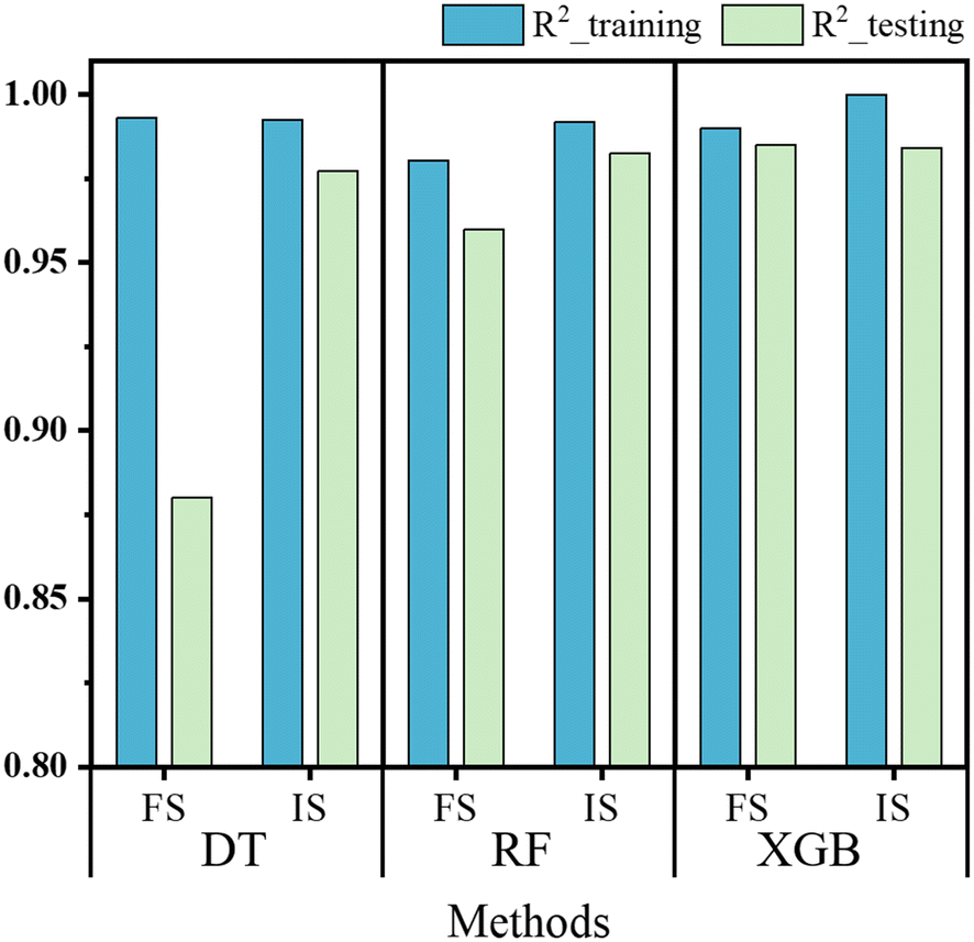Fig. 3 R ² score of the three models for predicting FS and IS on training and testing datasets.

This phenomenon could be attributed to the work process of the tree model, as illustrated in Fig. 4. This picture visualized the decision-making process of the DT model when predicting flexural strength. At the root node of the tree, the initial criterion is whether the value of crystallinity (Xc) is greater than 43.69, which divides the training dataset into two distinct subsets with significantly different flexural strengths. One subset contains 14 samples with a lower mean FS value of 15.38, while the other comprises 8 samples with a higher mean FS value of 25.54. This implies that higher crystallinity corresponds to higher polymer flexural strength. The DT model then continues to dichotomize the subset according to different ranges of polymer structure characteristics, following a strategy of minimizing differences in FS within the subset samples until the stopping condition is reached. The stopping condition is determined by hyperparameters, such as the maximum depth, which governs the growth of the decision tree. A greater depth leads to a more detailed classification, which may result in overfitting. The situation is exacerbated when the dataset is small in size.

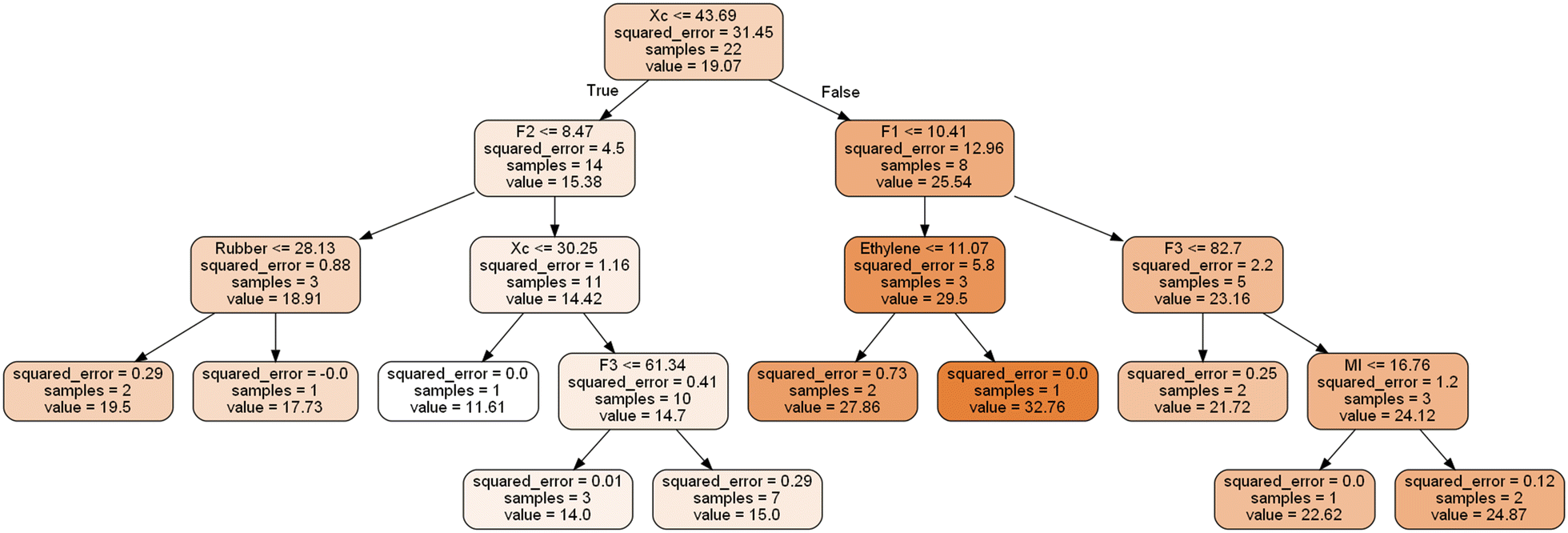Fig. 4 Visualization of the Decision Tree process for predicting flexural strength. Each box represents a node in the decision tree, containing decision criteria, squared error, sample count, and associated predicted values.

The limitations associated with a single decision tree can be mitigated by using ensemble models. RF is a classic ensemble machine learning technique that combines multiple decision trees in parallel. These trees are created using bootstrapped subsets of the training data. The term “Random” refers to the practice of randomly sampling data with replacement when creating each tree, and during tree splitting, a random subset of features is considered for decision-making. Each tree is trained independently and the output of each tree is taken into account. For regression problems, the final output of the “Forest” is determined by averaging the output of all trees. Consequently, Random Forest is less prone to overfitting. As depicted in Fig. 3, compared to the DT model, the RF model displays a narrower difference in R² score between the training and testing datasets.

XGB is also an ensemble model based on tree models, integrated using the boosting method. Different from the RF model, the XGB model creates multiple trees sequentially, as opposed to in parallel. Each tree in XGB is built based on the performance of all the preceding trees, aiming to minimize the prediction error through multiple iterations. This is achieved by adjusting the structure of the next tree using the gradient boosting algorithm. Fig. 5 displays three trees selected from the ensemble of 29 trees in the XGB model for predicting FS. Note that the values in each leaf of the next tree are generally lower than those in the previous tree, while the tree structure becomes more complex. The final output of XGB is determined by summing the predicted values for the corresponding leaf nodes across all trees. This implies that the predictions are continually adjusted as each tree is added. In addition, the XGB algorithm introduces regularization terms L1 and L2 into the model to mitigate the risk of overfitting, while reducing model complexity and consequently accelerating the solving process. XGB performed slightly better than RF with lower RMSE and a higher R² score when predicting FS and IS.

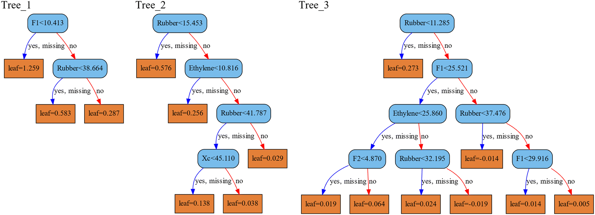Fig. 5 Three trees selected in the XGB model for flexural strength prediction. Blue boxes represent the decision criteria, while orange boxes indicate predicted values following decisions made on each tree.

3.2. Influence of structure features on material properties

As described above, XGB outperforms the other two algorithms and provides the most accurate predictions. Therefore, the analysis of the relationship between the polymer structural features and mechanical properties is based on the XGB model. To analyse feature importance in a model, SHAP values were utilized. SHAP values provide a more localized interpretation by pinpointing the average contribution of each feature, calculated by considering all possible combinations of feature permutations.³⁵

The SHAP values for Run1 and Run2 in the XGB model predicting FS are visualized in Fig. 6. The SHAP values reflect the local contribution of each feature from the sample mean to the model's predicted value. Among all the features, Rubber has the highest absolute SHAP value, with a value of 3.58 in Fig. 6(a), while it registers a negative value of −2.25 in Fig. 6(b). The larger the absolute value of SHAP, the higher the importance of the feature. A positive value indicates that the feature has a positive impact on the outcome, while a negative value indicates that the feature has a negative impact on the outcome. This implies that the rubber phase content significantly influences the flexural strength for Run1 and Run2. Specifically, when the rubber phase content is at 16.23 wt%, it contributes positively to the flexural strength, leading to an increase. Conversely, when the rubber phase content is at 31.75 wt%, it contributes negatively, resulting in a decrease in flexural strength.

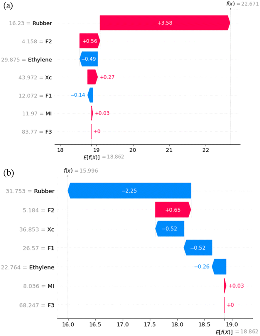Fig. 6 SHAP values for each feature in the XGB model predicting FS: (a) Run1 and (b) Run2.

The average absolute SHAP values for the entire training dataset and the SHAP values for each individual data point are depicted in Fig. 7. In this figure, (a) and (b) correspond to FS, while (c) and (d) pertain to IS. When considering the entire training dataset, the average absolute SHAP values provide insights into the importance of each feature. In the context of flexural strength (Fig. 7(a)), it is evident that the rubber phase content has the most substantial impact. The features F1, F2, Xc, and Ethylene exhibit relatively similar effects, all of which are less influential than rubber. Conversely, both MI and F3 have minimal influence on flexural strength.

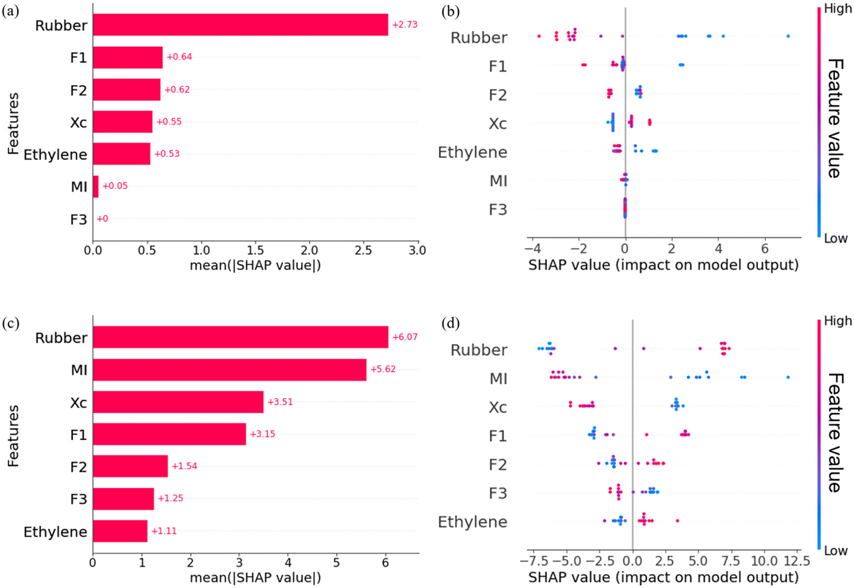Fig. 7 (a) Mean absolute SHAP values of each feature and (b) SHAP values of each data in XGB predicting FS; (c) mean absolute SHAP values of each feature and (d) SHAP values of each data in XGB predicting IS.

In Fig. 7(b), each dot represents the contribution of a specific feature to flexural strength. The colour of these dots corresponds to the values of the respective feature, with red indicating higher values and blue denoting lower values. Clearly, the rubber content has a significant impact on flexural strength, both at high and low levels. However, as the rubber content increases from low (blue dots) to high (red dots), its contribution to flexural strength changes from positive to negative. Additionally, when the dots for F1, F2, and Ethylene are red, and the dots for Xc are blue, the SHAP values are negative. This suggests that higher contents of ethylene–propylene random copolymer, ethylene–propylene segmented copolymer, and ethylene units in the polymer chain, as well as lower values of crystallinity, have a detrimental effect on the flexural strength.

For the impact strength, based on the SHAP value, Rubber is identified as the most influential feature, followed by MI, which has a slightly lower influence than Rubber. Next in order of influence are Xc, F1, F2, F3, and Ethylene features. In contrast to flexural strength, an increase in Rubber and a decrease in MI lead to an improvement in impact strength. As shown in Fig. 7(d), the SHAP values shift from negative to positive as the dots for Rubber transition from blue to red and the dots for MI from red to blue. Indeed, a low value of melt index, corresponding to a high positive SHAP value, indicates that a higher molecular weight is favourable for improving impact strength. An increase in Xc, resulting in a negative contribution, implies that high crystallinity in the polymer alloy has an adverse effect on the impact strength. Besides, higher contents of ethylene–propylene random copolymer, ethylene–propylene segmented copolymer, and ethylene units are advantageous for enhancing the impact strength of polymer alloys.

3.3. Effect of process conditions on the polymer rubber phase

From the above conclusion, the rubber phase content in the polymer alloy significantly affects both the flexural strength and impact strength. Therefore, the objective of this section is to explore the correlation between the rubber phase content and process conditions, as well as the strategies for controlling the rubber phase. To achieve this, an XGB model was established for predicting the rubber content based on various process conditions.

In Fig. 8(a), the mean absolute SHAP values of each process condition are depicted. It is evident that the initial pressure (initial P) and the feed flowrate of mixture gas have the highest SHAP values, followed by the ratio of ethylene (C2 in), copolymerization time (time), and the ratio of propylene (C3 in) and hydrogen (H2 in). This suggests that the pressure at the initial gas copolymerization stage and the feed flowrate during the copolymerization process have a significant impact on the synthesis of the rubber phase in the alloy. Additionally, the ratio of ethylene and propylene in the mixture gas feed and the reaction time also play important roles in determining the rubber phase content. In essence, the initial pressure also governs the ratio of ethylene and propylene in the gas reactor at the initial period of copolymerization. When the initial pressure is low, more ethylene needs to be initially fed into the reactor to reach the desired reaction pressure. This leads to a higher initial proportion of ethylene in the copolymerization reaction. Additionally, the feed flowrate impacts the rate at which gas concentrations are refreshed inside the reactor, with a higher feed flowrate resulting in faster updates of gas concentrations. These factors have significant implications for the synthesis of the rubber phase content in the alloy.

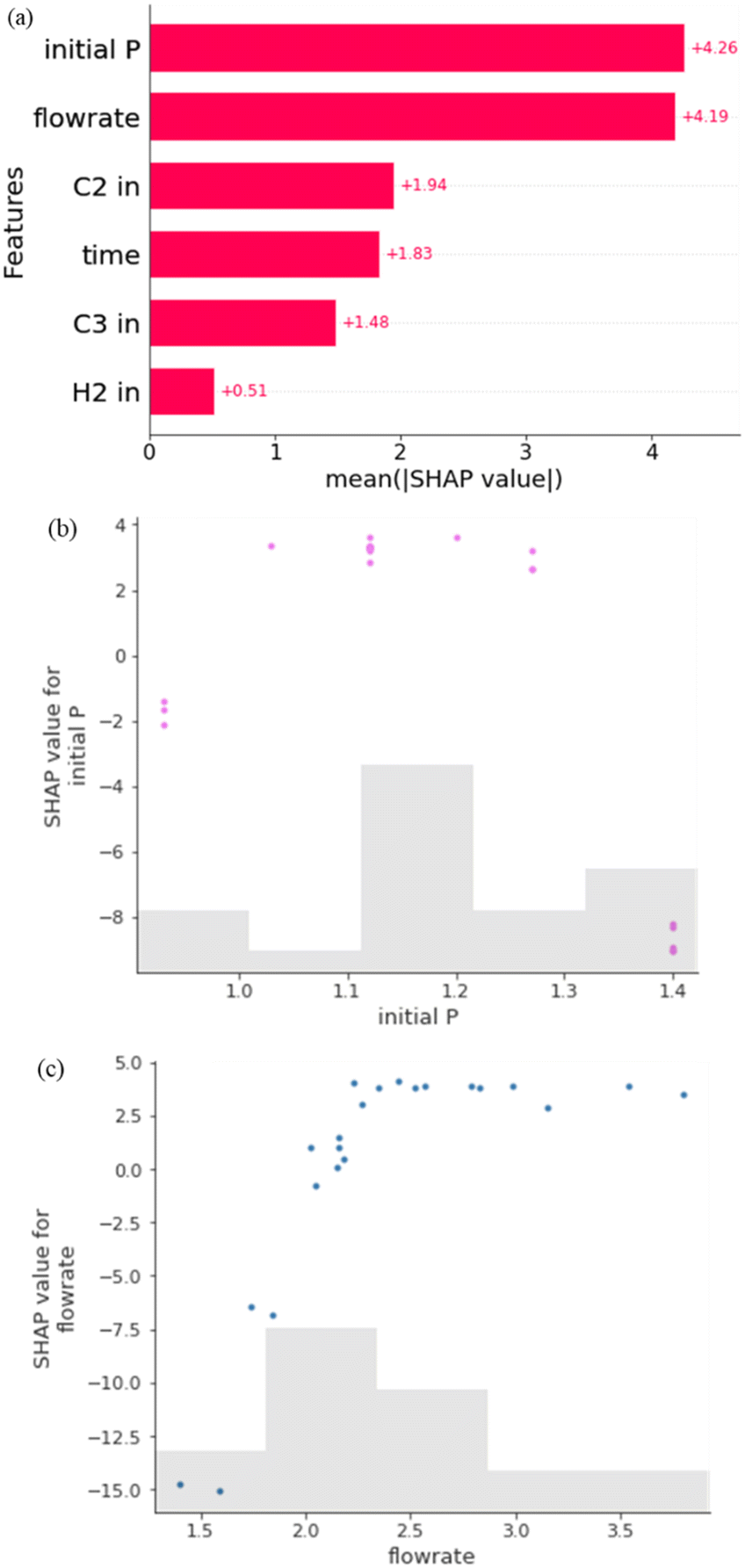Fig. 8 (a) Mean absolute SHAP values of process conditions in XGB predicting the rubber phase content; (b) SHAP value for the initial P vs. initial P; (c) SHAP value for the flowrate vs. flowrate.

In Fig. 8(b), the SHAP values for various individuals from the training dataset show how the importance attributed to the feature “initial P” changes as its value varies. The shadow represents the number of points in that interval. It indicates that when the initial pressure is at a moderate level, the SHAP value is high, while it decreases for both smaller and larger initial pressure values. This indicates that maintaining an appropriate initial pressure is beneficial for increasing the rubber phase content in the alloy. In Fig. 8(c), as the flowrate value increases, the SHAP value for the flowrate increases and then stabilizes, suggesting that a larger feed flowrate of mixture gas can enhance the rubber phase content.

3.4. Predicting mechanical properties through process conditions

Both the relationship between the polymer structure and performance, and the influence of process conditions on the structure have been elucidated. Therefore, it is possible to directly predict polymer properties from process conditions. Fig. 9 displays the parity plots of the XGB model predicting flexural and impact strength based on process conditions. The model exhibits strong performance, with data points from both the training and testing datasets closely aligned with the black line. The R² scores of FS are above 0.99 and 0.95 for the training and testing datasets, respectively, while for IS, they exceed 0.99 and 0.97. Furthermore, the errors are relatively small, with FS having RMSE values of 0.2765 and 0.7341 for the training and testing datasets, respectively, and IS having RMSE values of 0.7286 and 3.2383. The result indicates that the model exhibits good fitting and generalization capabilities, making it suitable for predicting both flexural and impact strength.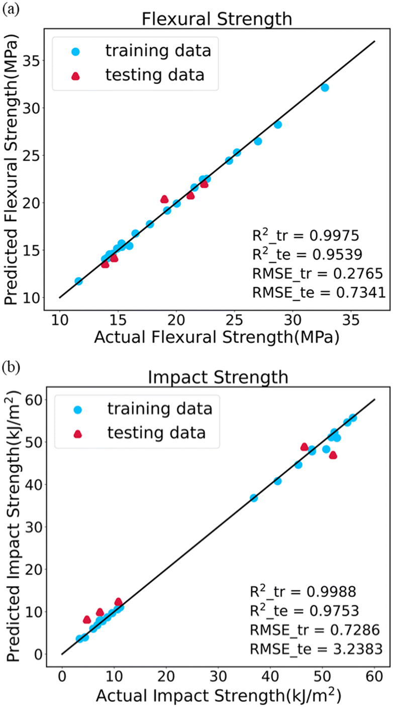

Fig. 9 Parity plots of XGB using process conditions to predict two mechanical properties: (a) FS and (b) IS.

The SHAP values for each process condition are presented in Fig. 10. It is clear that the flowrate and initial P have the most significant influence on both FS and IS. A low mixed gas feed flowrate and a higher initial pressure have a positive contribution to FS, while a larger mixed gas feed flowrate and a moderate initial pressure have proven beneficial for IS. These observed effects can be attributed to the changes induced by these specific process conditions, resulting in variation in the rubber phase content in the alloy and subsequently influencing the physical properties. This is consistent with the established correlation between the polymer structure and properties, and the impact of process conditions on structural characteristics, as previously elucidated.

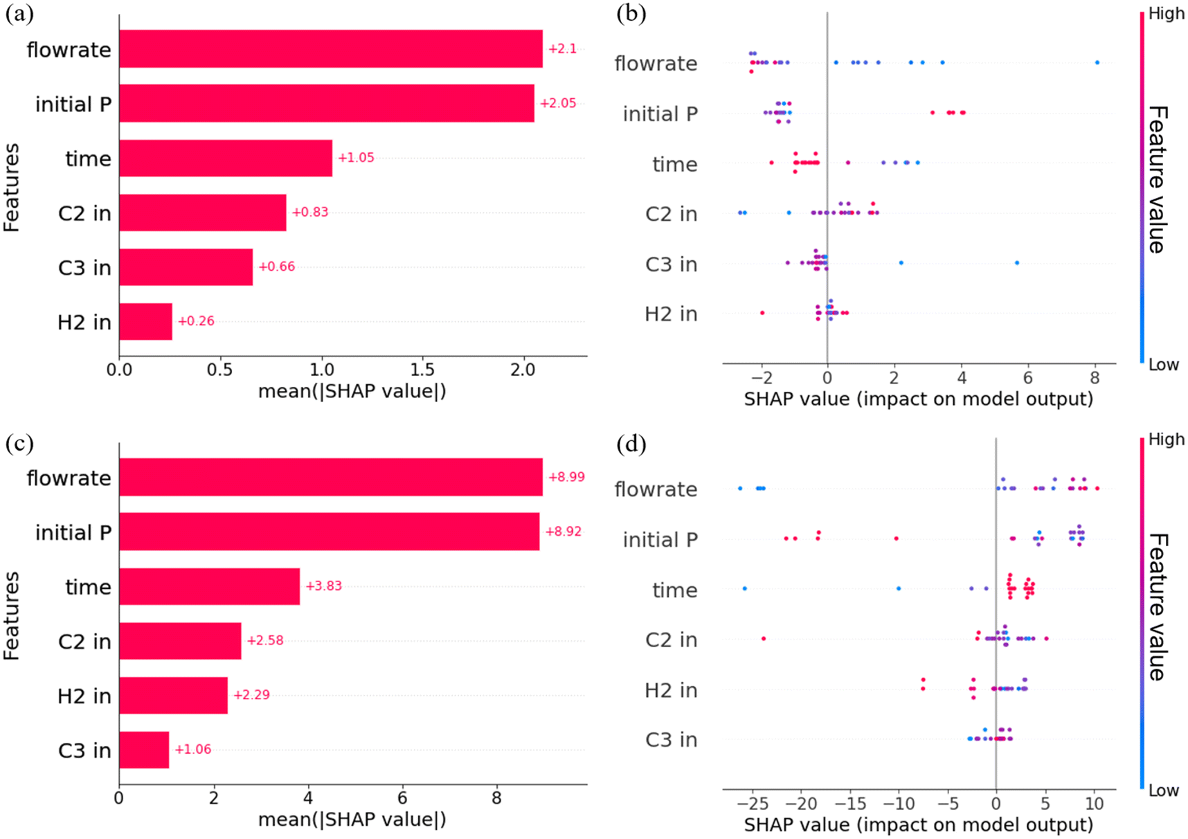Fig. 10 (a) Mean absolute SHAP values of process conditions and (b) SHAP values of each data in XGB predicting FS; (c) mean absolute SHAP values of process conditions and (d) SHAP values of each data in XGB predicting IS.

To further validate the accuracy of the established model in predicting mechanical properties, five experimental runs were designed, each involving various process conditions. In light of the previous feature importance analysis, particular attention was paid to the variation of the flowrate. The flowrate was varied over a wide range with five different values to ensure that these experimental protocols are as distinct as possible from the training and testing data mentioned previously. In addition, the values of flowrate are all higher than 2.5 kg h⁻¹ because a high flowrate is beneficial for impact strength, which is the primary goal of PP alloys. The XGB model was also employed to generate predicted values for these conditions. The predictions for FS and IS and the corresponding experimental values are listed in Table 3.

Table 3 The process conditions of gas-phase copolymerization, model predicted FS and IS values and experimental values

Entry	C2 in	C3 in	H2 in	Initial P (MPa)	Flowrate (kg h^−1)	Time (min)	Predicted FS (MPa)	Experimental FS (MPa)	Predicted IS (kJ m^−2)	Experimental IS (kJ m^−2)
Run 28	0.398	0.595	0.007	1.12	2.93	60	17.08	15.70	52.69	45.00
Run 29	0.395	0.598	0.007	1.12	2.56	75	13.13	14.71	52.09	47.47
Run 30	0.396	0.599	0.005	1.12	2.61	75	14.86	14.39	55.95	52.22
Run 31	0.405	0.590	0.005	0.93	3.18	75	15.35	13.24	55.51	55.89
Run 32	0.403	0.592	0.005	0.93	3.66	75	15.35	15.86	55.51	53.14

---

The experimental results closely aligned with the model's prediction for both flexural strength and impact strength, yielding RMSE values of 1.3656 and 4.4751, respectively. Although these RMSE values are slightly elevated compared to the model's performance on the training and testing datasets, it is worth noting that the XGB model still delivers satisfactory prediction for the uncharted experimental conditions. Furthermore, all newly designed experimental protocols yielded satisfactory impact strength values.

Conclusions

This study explores the relationship between the process conditions, polymer structure, and mechanical properties of polypropylene in-reactor alloys using machine learning techniques. The research leveraged quantitative data gathered from the polymerization process and polymer characterization to build datasets for machine learning models. Three different algorithms were employed to develop regression models aimed at predicting mechanical properties based on the polymer structure. Among these algorithms, the XGB model exhibited superior performance with higher R² scores and lower RMSE values. By analysing SHAP values, the study identified that the rubber phase content significantly influences flexural strength, while both the rubber phase content and melt index have a substantial impact on impact strength. Furthermore, the research uncovered the relationship between the process conditions and rubber phase content using XGB algorithms to create predictive models. The results highlighted the critical roles of the flowrate and initial pressure in rubber synthesis, which in turn affect flexural strength and impact strength. To validate the model's accuracy, new experimental runs were designed to synthesize alloys for achieving improved impact strength. The experimental results closely matched the predictions from the model. This research offers a novel approach to establish the process–structure–property relationship for polypropylene in-reactor alloys and provides a convenient method for designing experiments to achieve desired material mechanical properties, saving valuable research time.

Author contributions

Shaojie Zheng designed and conducted the experiments and modelling under the guidance of Yao Zhen and Jijiang Hu. Shaojie Zheng and Xu Huang performed the experimental characterization. Yao Zhen and Jijiang Hu supported the project with their expertise. Shaojie Zheng wrote the manuscript, and Zhen Yao conducted the revisions. All authors participated in result discussions and manuscript review.

Conflicts of interest

The authors declare that they have no known competing financial interests or personal relationships that could have appeared to influence the work reported in this paper.

Acknowledgements

The authors are grateful to the National Natural Science Foundation of China for their support through NSFC Project #: 21938010.

References

1. Y. Liu, B. Zhang, Z. Fu and Z. Fan, Macromol. Res., 2017, 25, 534.
2. R. Mehtarani, Z.-S. Fu, S.-T. Tu, Z.-Q. Fan, Z. Tian and L.-F. Feng, Ind. Eng. Chem. Res., 2013, 52, 9775.
3. B. Zhang, W. Zhong, Z. Fu and Z. Fan, Eur. Polym. J., 2021, 154, 110563.
4. L. Moballegh, S. Hakim, J. Morshedian and M. Nekoomanesh, J. Polym. Res., 2015, 22, 1.
5. X. Wang, R. Xu, W. Kang, J. Fan, X. Han and Y. Xu, Polymers, 2020, 12, 751.
6. C. Jiang, B. Jiang, Y. Yang, Z. Huang, Z. Liao, J. Sun, J. Wang and Y. Yang, Polymer, 2021, 214, 123373.
7. W. Liu, J. Zhang, M. Hong, P. Li, Y. Xue, Q. Chen and X. Ji, Polymer, 2020, 188, 122146.
8. Z. Tian, X.-P. Gu, G.-L. Wu, L.-F. Feng, Z.-Q. Fan and G.-H. Hu, Ind. Eng. Chem. Res., 2011, 50, 5992.
9. W. Wang, W. Zhang and B. Liang, J. Mater. Sci., 2021, 56, 15667.
10. M. T. Pastor-García, I. Suárez, M. T. Expósito, B. Coto and R. A. García-Muñoz, Eur. Polym. J., 2021, 157, 110642.
11. H. Xu, S. Ma, Y. Hou, Q. Zhang, R. Wang, Y. Luo and X. Gao, ACS Appl. Mater. Interfaces, 2022, 14, 47157.
12. K. Sharifani and M. Amini, World Information Technology Engineering Journal, 2023, 10, 3897.
13. P. Xu, H. Chen, M. Li and W. Lu, Adv. Theory Simul., 2022, 5, 2100565.
14. J. Vamathevan, D. Clark, P. Czodrowski, I. Dunham, E. Ferran, G. Lee, B. Li, A. Madabhushi, P. Shah and M. Spitzer, Nat. Rev. Drug Discovery, 2019, 18, 463.
15. C. Li, G. Zhang, S. Mohapatra, A. J. Callahan, A. Loas, R. Gómez-Bombarelli and B. L. Pentelute, Adv. Sci., 2022, 9, 2201988.
16. F. Castéran, R. Ibanez, C. Argerich, K. Delage, F. Chinesta and P. Cassagnau, Macromol. Mater. Eng., 2020, 305, 2000375.
17. R. Bhowmik, S. Sihn, R. Pachter and J. P. Vernon, Polymer, 2021, 220, 123558.
18. C. Joo, H. Park, J. Lim, H. Cho and J. Kim, Int. J. Intell. Syst., 2021, 37, 3625.
19. C. Joo, H. Park, H. Kwon, J. Lim, E. Shin, H. Cho and J. Kim, Polymers, 2022, 14, 3500.
20. P. Xu, X. Ji, M. Li and W. Lu, npj Comput. Mater., 2023, 9, 42.
21. R. Cai, K. Wang, W. Wen, Y. Peng, M. Baniassadi and S. Ahzi, Polym. Test., 2022, 110, 107580.
22. D. Kamireddi, A. Terapalli, V. Sridevi, M. T. Bai, D. V. Surya, C. S. Rao and L. R. Jeeru, J. Anal. Appl. Pyrolysis, 2023, 172, 105984.
23. F.-Y. Wu, J. Yin, S.-C. Chen, X.-Q. Gao, L. Zhou, Y. Lu, J. Lei, G.-J. Zhong and Z.-M. Li, Polymer, 2023, 269, 125736.
24. G. Liu, P. Wei, K. Chen, H. Liu and Z. Lu, J. Comput. Des. Eng., 2022, 9, 583.
25. L. Li, S. Kumar Damarla, Y. Wang and B. Huang, Inf. Sci., 2021, 581, 262.
26. D. Li, J. Liu and J. Liu, Macromol. Theory Simul., 2021, 30, 2100010.
27. L. Shen and Q. Qian, Comput. Mater. Sci., 2022, 211, 111475.
28. B. Zhang, Z. Fu, Z. Fan, P. Phiriyawirut and S. Charoenchaidet, J. Appl. Polym. Sci., 2016, 133, 42984.
29. Z. Tian, L.-F. Feng, Z.-Q. Fan and G.-H. Hu, Ind. Eng. Chem. Res., 2014, 53, 11345.
30. Y.-Y. Song and L. Ying, Shanghai Arch. Psychiatry, 2015, 27, 130.
31. L. Breiman, Mach. Learn., 2001, 45, 5.
32. T. Chen and C. Guestrin, Presented in Part at the Proceedings of the 22nd ACM SIGKDD International Conference on Knowledge Discovery and Data Mining, 2016.
33. S. M. Lundberg and S.-I. Lee, Presented in part at the 31st Conference on Neural Information Processing Systems (NIPS 2017), Long Beach, CA, USA, 2017.
34. S. M. Lundberg, G. G. Erion and S.-I. Lee, arXiv, 2018, preprint, 03888,  DOI:10.48550/arXiv.1802.03888.
35. J. Jeon, B. Rhee and J. Gim, Polymers, 2022, 14, 5548.

---

Footnote

† Electronic supplementary information (ESI) available. See DOI: https://doi.org/10.1039/d3re00504f

---