
 Open Access Article
 This Open Access Article is licensed under a Creative Commons Attribution-Non Commercial 3.0 Unported Licence
Gas-phase errors in computational electrocatalysis: a review
Ricardo
Urrego-Ortiz
 ab,
Santiago
Builes
c,
Francesc
Illas
a and
Federico
Calle-Vallejo
*bd
ab,
Santiago
Builes
c,
Francesc
Illas
a and
Federico
Calle-Vallejo
*bd
aDepartament de Ciència de Materials i Química Física & Institut de Química Teòrica i Computacional (IQTCUB), Universitat de Barcelona, C/ Martí i Franquès 1, 08028 Barcelona, Spain
bNano-Bio Spectroscopy Group and European Theoretical Spectroscopy Facility (ETSF), Department of Polymers and Advanced Materials: Physics, Chemistry and Technology, University of the Basque Country UPV/EHU, Av. Tolosa 72, 20018 San Sebastián, Spain. E-mail: federico.calle@ehu.es
cEscuela de Ciencias Aplicadas e Ingeniería, Universidad EAFIT, Carrera 49 # 7 sur 50, 050022, Medellín, Colombia
dIKERBASQUE, Basque Foundation for Science, Plaza de Euskadi 5, 48009 Bilbao, Spain
First published on 29th September 2023
Abstract
Currently, computational models based on density functional theory (DFT) are intensively used for the analysis of electrocatalytic reactions and the design of enhanced catalysts. As the accuracy of these models is subjected to the quality of the input data, knowing the intrinsic limitations of DFT is crucial to improve computational predictions. A common pitfall of DFT is the estimation of the total energies of molecules, particularly those containing double and triple bonds. In this review, we show how gas-phase errors permeate thermodynamic and kinetic models of customary use in electrocatalysis, potentially compromising their predictiveness. First, we illustrate how these errors can be identified and provide a list of corrections for common molecules and functional groups. Subsequently, we explain how the errors spread from simple reaction energy calculations to adsorption energies, scaling relations, equilibrium potentials, overpotentials, and Sabatier-type activity plots. Finally, we list the remaining challenges toward an improved assessment of energetics at solid–gas–liquid interfaces.
 Ricardo Urrego-Ortiz | Ricardo Urrego-Ortiz received his BSc degree in Process Engineering from EAFIT University (Colombia) in 2017. Later, he worked as a project engineer and data scientist in a company focused on energy efficiency. In 2021, Ricardo obtained his MSc in engineering at EAFIT University. Currently, he is a PhD student at the University of Barcelona funded by “la Caixa” Foundation. Ricardo uses theoretical chemistry and computational tools to address major societal and environmental challenges, such as the imbalance of the nitrogen and carbon cycles, and the transition from fossil fuels toward sustainable energy sources. |
 Santiago Builes | Santiago Builes is a professor of process engineering at EAFIT University (Colombia). He received his PhD degree (2012) in materials science from the Autonomous University of Barcelona (Spain). Afterwards, he was a postdoctoral researcher at the University of Delaware (USA). Santiago applies molecular modeling and computational chemistry to address environmental challenges and obtain a better understanding of industrial processes. His research focuses on atomistic simulations of separation processes and (electro)catalysis, in areas such as carbon capture and utilization. |
 Francesc Illas | Francesc Illas is a Full Professor of Physical Chemistry at the University of Barcelona. He spent several periods at IBM Almaden Research Center and Los Alamos National Laboratory and was invited professor at Universita’ della Calabria (Italy) and Université Pierre et Marie Curie (France). He has received several awards, was elected Fellow of the European Academy of Sciences (2009), of the Academia Europeae (2017) and is the recipient of the 2022 Medal of the Spanish Royal Society of Chemistry. His research involves the application of theoretical and computational chemistry methods to surface chemistry and heterogeneous catalysis. |
 Federico Calle-Vallejo | After his degree in chemical engineering in Colombia, Federico Calle-Vallejo did his PhD at DTU (Denmark) and was a postdoctoral researcher at Leiden University (the Netherlands) and ENS Lyon (France). Subsequently, he was a Veni research fellow at Leiden University and a Ramón y Cajal research fellow at the University of Barcelona (Spain). Currently, Federico Calle-Vallejo is an Ikerbasque Research Associate and Visiting Professor at the University of the Basque Country (Spain). Federico's group uses DFT and in-house methods and descriptors to make predictive models of electrocatalytic reactions with structural and compositional sensitivity. |
Broader contextThe massive emissions of oxidized carbon and nitrogen species urgently call for an energetic transition that restores the balance to the biogeochemical cycles of those two elements. Electrochemical technologies such as electrolyzers are prominent alternatives to drive such a transition as they use electrical power from renewable sources to convert C- and N-containing pollutants into valuable feedstocks. However, electrochemical technologies currently rely on catalysts based upon scarce and expensive elements, which has motivated an intensive search for alternative materials preferably composed of earth-abundant elements. Computational models based on density functional theory (DFT) are extensively used for this purpose thanks to their reasonable tradeoff between accuracy and affordability. Nevertheless, DFT calculations usually entail large errors when predicting the energy of countless gaseous molecules commonly found as reactants and products of electrocatalytic reactions. In this review, we show how to detect and correct these errors in the gas phase, so as to prevent their spread over computational electrocatalysis models. The negative impact of these errors on the predictive power of electrocatalysis models is illustrated for a variety of reactions belonging to the carbon and nitrogen cycles. |
1. Introduction
Contemporary computational electrochemistry has fostered a new era in the design of catalytic materials at the atomic scale.1–5 Ever since the pioneering works of Nørskov, Rossmeisl and coworkers, DFT-based electrochemical models have been extensively used to study and design efficient catalysts for key reactions in sustainable development, such as hydrogen evolution, oxygen reduction and evolution, and the production of fuels and commodity chemicals from CO2.5–11 Nowadays, computational electrochemistry is a prominent tool to address the colossal challenges of climate change and the much-needed energy transition.4The reliability of DFT-based computational models depends on the method employed to approximate the exact but unknown universal exchange–correlation functional (xc-functional). This poses an often unnoticed but important constraint in heterogeneous (electro)catalysis where gas–liquid–solid interfaces ought to be suitably described, which is hardly achieved by a single functional chosen among the existing families.12,13 For instance, hybrid functionals are widely used to accurately predict molecular properties but fail in the description of metals,14–16 whereas affordable functionals at the generalized gradient approximation (GGA) provide fair results for conductive solids and surfaces but possess serious limitations for gases, such as the well-known overbinding of O2 and N2.17–19 Meta-GGA functionals supposedly improve the deficiencies of GGAs for molecules while maintaining the accuracy for solids and surfaces, but their use in (electro)catalysis is still incipient due to their high computational cost, convergence problems, and because they have not been shown yet to outperform GGA functionals in terms of chemisorption.18,20,21
Although gas-phase errors in GGA functionals have been exposed using datasets containing mainly small molecules,22–24 recent works show that such errors also permeate meta-GGA and hybrid functionals for the prediction of thermodynamic properties of molecules with environmental and industrial relevance, such as nitrates, carboxylic acids and several other families of organic compounds, and hydrogen peroxide.25–29 This implies that accurate estimations of basic properties and parameters in electrocatalysis, such as adsorption/desorption energies and equilibrium potentials, are not guaranteed by simply climbing the so-called Jacob's ladder of accuracy.30 In fact, accurate predictions may rely on error cancellation more often than we think, which occurs when the DFT errors of the reactants and products are similar.31–33 This condition is not always met, as attested by the CO2 reduction to CO and numerous reactions among nitrogen oxides,25,34 so it is advisable to assess the gas-phase errors of each compound separately.
Because DFT-based models have become customary in (electro)catalysis and most often use GGA functionals, it is crucial to assess the impact of gas-phase errors on their predictiveness. In this review, we first summarize various methods for identifying and quantifying these errors. Next, we explain how they affect calculated properties ranging from simple equilibrium potentials and adsorption energies to more complex Sabatier-type analyses based on scaling relations and volcano plots. Finally, we provide a brief overview of the challenges lying on the way toward an accurate DFT modeling of electrocatalytic reactions involving molecules at surfaces.
2. Detection and quantification of DFT gas-phase errors
2.1 Basic error formulations
For a reaction in the gas phase, the enthalpy (ΔrHDFT) and Gibbs energy (ΔrGDFT) change can be estimated from DFT calculations using the following equations: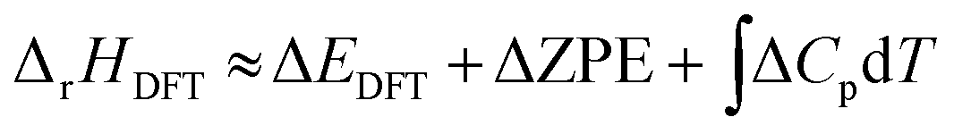 | (1) |
| ΔrGDFT = ΔrHDFT − TΔS | (2) |
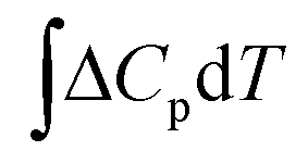 is the change in the heat capacity contribution, which is usually neglected because of the cancellation of the contributions of products and reactants in the range of 0 to 298.15 K.6,28,35 However, we anticipate that this term may not be negligible for reactions with numerous proton–electron transfers. In eqn (2), TΔS represents the difference between the total entropies of the products and reactants, usually taken from thermodynamic tables.1,36
Eqn (1) and (2) can be compared to the corresponding experimental values (ΔrHexp and ΔrGexp, respectively), thus allowing to define a total DFT error (εT) as per eqn (3).25,34
| εT = ΔrGDFT − ΔrGexp = ΔrHDFT − ΔrHexp | (3) |
 | (4) |
Finally, we note that convergence tests are usually carried out to rule out that gas-phase errors come from an inadequate selection of the setup of the DFT calculations. For plane-wave codes, this is ensured by showing that the variations in the Gibbs energy of a prototypical reaction are within 0.05 eV as a function of the plane-wave energy cutoff.25,27,28,34,42
2.2 Pinpointing individual errors
Numerous studies have exposed significant DFT errors for several molecules in the gas phase using different xc-functionals,23,43–49 and ΔEDFT has been identified as the main error source since the ZPEs are generally in line with experiments,29 simply because the harmonic calculated vibrational frequencies are generally rather accurate. As reasonable predictions of gas-phase energetics should not rely on error cancellation, namely when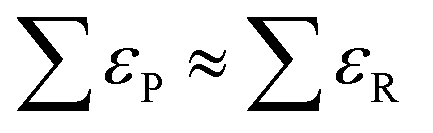 in eqn (4), significant efforts have recently been devoted to pinpoint and estimate the errors in ΔEDFT of gaseous compounds in a systematic manner. The most common methods are the following:
To identify if a molecule or certain chemical structure is a potential source of error, the authors collected several reactions involving that molecule/structure and available experimental reaction enthalpy data. Then, the DFT-calculated energies of those reactions were compared to the experimental ones and the mean absolute error (MAE) calculated. A statistical analysis was performed by artificially varying the DFT-calculated energy (EDFT) of the “problematic” molecule until the MAE was minimized. The difference between the value that minimizes the MAE and the calculated DFT energy of the molecule is taken as its error. Statistical analyses can be performed simultaneously for multiple compounds or structures provided that the set of chemical reactions is sufficiently large and experimental data are available.
Using this approach, the authors found large PBE errors for CO (−0.51 eV) and large RPBE errors for CO2 (0.45 eV) and proposed the OCO backbone as a problematic group of atoms that affects numerous compounds in the carbon cycle for RPBE, including carboxylic acids and esters. In Fig. 1a, the sensitivity analysis used to obtain the RPBE error of the OCO backbone is presented: the MAE is minimized when an error of 0.45 eV is assigned to the compounds including an OCO backbone in their structure. The MAE of bystander reactions, that is the reactions that do not involve OCO-containing species, remains constant upon applying the corrections.
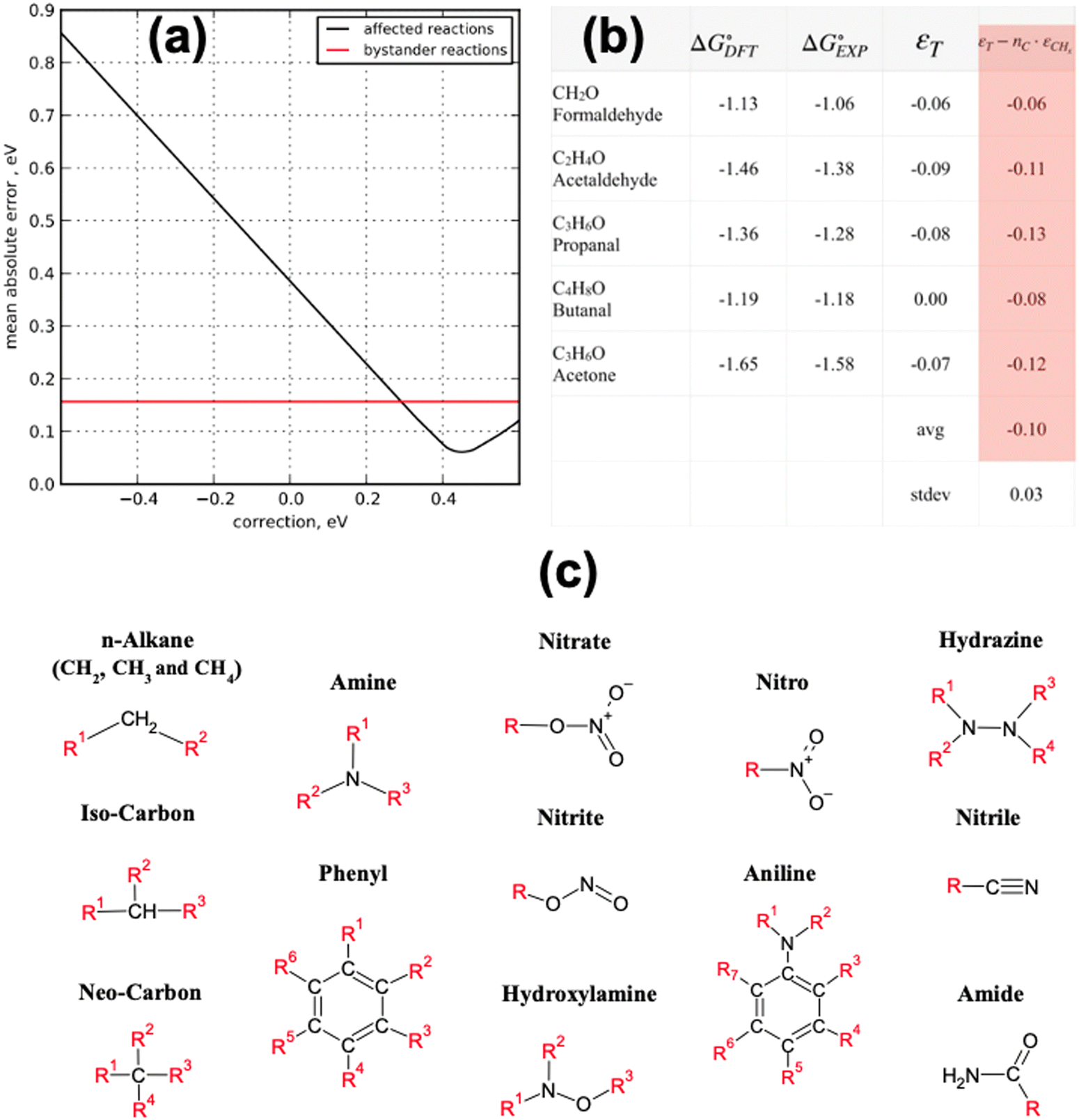 | ||
Fig. 1 Summary of the statistical methods that use experiments as a reference to identify and quantify the errors in the DFT energy of gas-phase compounds. (a) The black line shows the MAE minimization through sensitivity analysis of the OCO backbone error for RPBE for reactions involving CO2, HCOOH, CH3COOH and HCOOCH3. In red, the unaffected MAE of reactions not involving OCO-containing molecules. Reproduced from ref. 6 Copyright 2010, Royal Society of Chemistry. (b) Determination of the carbonyl group (–C![[double bond, length as m-dash]](https://www.rsc.org/images/entities/char_e001.gif) O–) error in PBE from a dataset of 5 molecules, considering that alkane groups (CHx) also contribute to the total error. Reproduced from ref. 34, licensed under CC-BY-NC-ND (https://creativecommons.org/licenses/by-nc-nd/4.0/). (c) Functional groups with appreciable DFT errors in organic compounds. Adapted from ref. 25 Copyright 2021, John Wiley and Sons. O–) error in PBE from a dataset of 5 molecules, considering that alkane groups (CHx) also contribute to the total error. Reproduced from ref. 34, licensed under CC-BY-NC-ND (https://creativecommons.org/licenses/by-nc-nd/4.0/). (c) Functional groups with appreciable DFT errors in organic compounds. Adapted from ref. 25 Copyright 2021, John Wiley and Sons. | ||
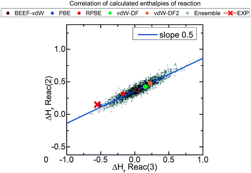
Along these lines, other studies have used experimental formation enthalpies and free energies to show that functional groups, as defined in organic chemistry, introduce systematic, additive errors.25,34Fig. 1b shows how the PBE error of the carbonyl group (–CO–) is obtained using a set of 5 molecules with known experimental formation energies after accounting for the respective linear alkane group error (–CHx),34 and Fig. 1c shows various C- and N-containing functional groups. The errors in those groups were estimated for four GGA functionals in a similar manner and are compiled in Table 1.
| Molecule or functional group | PBE | PW91 | RPBE | BEEF-vdW |
|---|---|---|---|---|
| a Errors obtained from ref. 26. Unmarked errors are taken from ref. 25. b Errors obtained from ref. 34. c Errors obtained from ref. 27. d Errors obtained from ref. 29. e The errors of NO3(aq)− and NO2(aq)− correspond to those of HNO3(g) and HNO2(g), respectively.50,51 | ||||
| O2a | −0.46 | −0.33 | −0.74 | −0.81 |
| N2 | 0.34 | 0.38 | −0.05 | −0.32 |
| CO2b | −0.19 | −0.15 | −0.46 | −0.56 |
| COb | 0.24 | 0.25 | −0.07 | −0.18 |
| H2O2c | −0.26 | −0.23 | −0.29 | −0.34 |
| NOd | −0.07 | 0.05 | −0.41 | −0.58 |
| NO2d | −0.80 | −0.66 | −1.12 | −1.27 |
| NO3d | −1.41 | −1.26 | −1.72 | −1.92 |
| N2Od | −0.50 | −0.41 | −0.86 | −1.10 |
| HNOd | −0.05 | −0.01 | −0.30 | −0.43 |
| HNO2d | −0.54 | −0.48 | −0.78 | −0.95 |
| HNO3d | −0.96 | −0.87 | −1.14 | −1.35 |
| NO2(aq)−de | −0.54 | −0.48 | −0.78 | −0.95 |
| NO3(aq)−de | −0.96 | −0.87 | −1.14 | −1.35 |
| cis-N2O2d | −0.71 | −0.55 | −1.25 | −1.59 |
| N2O3d | −1.19 | −1.06 | −1.66 | −2.04 |
| N2O4d | −1.80 | −1.63 | −2.22 | −2.62 |
| N2O5d | −2.04 | −1.86 | −2.42 | −2.87 |
| Amine, –NHx | 0.00 | 0.00 | 0.04 | −0.09 |
| Nitro, –NO2 | −0.65 | −0.57 | −0.81 | −1.08 |
| Nitrate, –NO3 | −1.00 | −0.91 | −1.17 | −1.45 |
| Nitrite, –ONO | −0.56 | −0.50 | −0.79 | −1.02 |
| Hydroxylamine, –(NHxOHy)– | −0.16 | −0.15 | −0.15 | −0.31 |
| Phenyl, –Ph | −0.06 | −0.12 | −0.13 | 0.17 |
| Aniline, –(N–Ph)– | −0.16 | −0.21 | −0.16 | 0.05 |
| Hydrazine, –(N–N)– | −0.09 | −0.08 | −0.05 | −0.21 |
| Amide, –(CO)NH2 |
−0.17 | −0.15 | −0.20 | −0.38 |
| Nitrile, –CN | 0.10 | 0.11 | −0.17 | −0.33 |
| n-Alkane*, –CHx | 0.036 | 0.015 | 0.086 | 0.203 |
| Iso-carbon alkane, –CH– | 0.13 | 0.12 | 0.25 | 0.20 |
| Neo-carbon alkane, –C– | 0.22 | 0.21 | 0.38 | 0.27 |
| Carbonyl, –CO–a |
−0.10 | −0.10 | −0.21 | −0.27 |
| Carboxyl, –(CO)O–a |
−0.19 | −0.19 | −0.27 | −0.34 |
| Hydroxyl, –OHa | −0.04 | −0.04 | −0.01 | −0.14 |
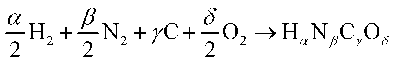
In this correction scheme, the DFT energies of two reactions obtained with different xc-functionals are compared. If a linear correlation is obtained, it is considered that at least one error source is present for all xc-functionals, namely an ill-represented molecule/chemical structure. The slope of such linear relation is rationalized as the change in the number of occurrences of the problematic molecule/structure in the y-axis reaction versus the change in the x-axis reaction. For example, Fig. 2 correlates the reaction enthalpies of H2 + CO2 → HCOOH (reaction (2)) and 3H2 + CO2 → CH3OH + H2O (reaction (3)) obtained with several xc-functionals. The authors used GGA functionals accounting or not for van der Waals (vdW) interactions, such as BEEF-vdW and PBE, and 2000 functionals obtained by varying the expansion coefficients of BEEF-vdW.52 Advantageously, this approach allows to predict errors in adsorbed species without using experimental heats of adsorption, which are scarce in the literature.21
 | ||
| Fig. 2 Correlations between the enthalpies of reactions 2 (H2 + CO2 → HCOOH) and 3 (3H2 + CO2 → CH3OH + H2O) calculated with ensembles of xc-functionals. Each color represents the result for a functional: PBE in blue, RPBE in red, vdW-DF in green, vdW-DF2 in orange, BEEF-vdW in black and outlined in red, and the ensemble of functionals obtained from BEEF-vdW are in gray. The red cross corresponds to the experimental value. Reproduced with permission from ref. 40, licensed under CC-BY 3.0 (https://creativecommons.org/licenses/by/3.0/)/Cropped from original. | ||
If the OCO backbone is assumed to be the main error source in the reactions of Fig. 2, a linear correlation with a slope of 0 is expected since the OCO backbone in the first reaction is preserved (it is present both in CO2 and HCOOH) while in the second reaction it is consumed, thus 0/−1 = 0. However, if the CO error is assumed to be dominant, the observed slope of 0.5 is obtained as only one of the two CO in CO2 is consumed in the first reaction (HCOOH preserves one CO), while the two CO are consumed in the second reaction, hence −1/−2 = 0.5. After identifying the CO bond as the main source of error, its individual correction could be obtained by comparison to experimental data following the approach described before in (i). Note in passing that the errors associated to adsorbed species can also be calculated for a given adsorbate and material by means of adsorption-energy scaling relations, as explained in detail in Section 5.39
 | (5) |
 | (6) |
 or Gibbs energies
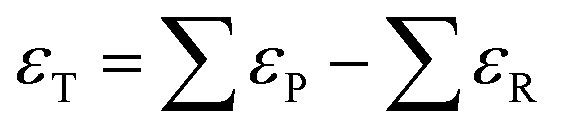
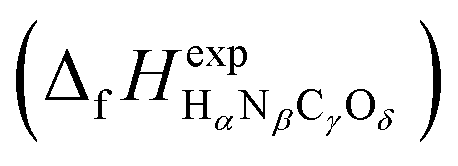
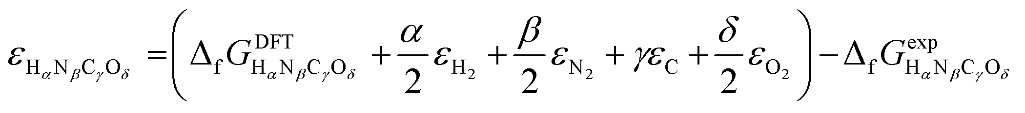
 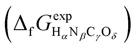 is facultative and usually depends on the availability of experimental data. In principle, the errors calculated from free energies and enthalpies should be identical. However, it is probably more advisable to make the error assessment on the basis of Gibbs energies, as they are connected to the equilibrium potentials of electrochemical reactions, see Section 3. Moreover, by means of eqn (4), the total error can be further decomposed into the difference between the errors of the reactants (H2, N2, C, and O2) and products (HαNβCγOδ) considering their stoichiometric coefficients given in eqn (5).
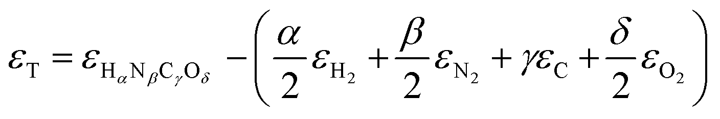 | (7) |
 | (8) |
Eqn (8) can be simplified by noting that DFT usually yields good predictions for hydrogen49 and graphene, which is often employed as the reference to model carbon instead of graphite due to the weak interlayer forces of the latter.53–58 Hence, εH2 ≈ εC ≈ 0. Furthermore, εO2 can be explicitly calculated from the water formation reaction 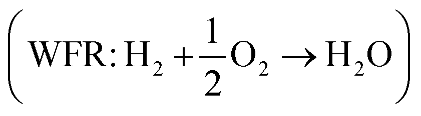 assuming that the error in the calculated energy of H2O is negligible,31 and εN2 from the ammonia synthesis reaction25
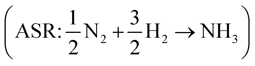 , as NH3 is also reasonably well described by DFT.49 From the WFR we obtain eqn (9), and the ASR yields eqn (10).
| εO2 = −2(ΔfGDFTWFR − ΔfGexpWFR) | (9) |
| εN2 = −2(ΔfGDFTASR − ΔfGexpASR) | (10) |
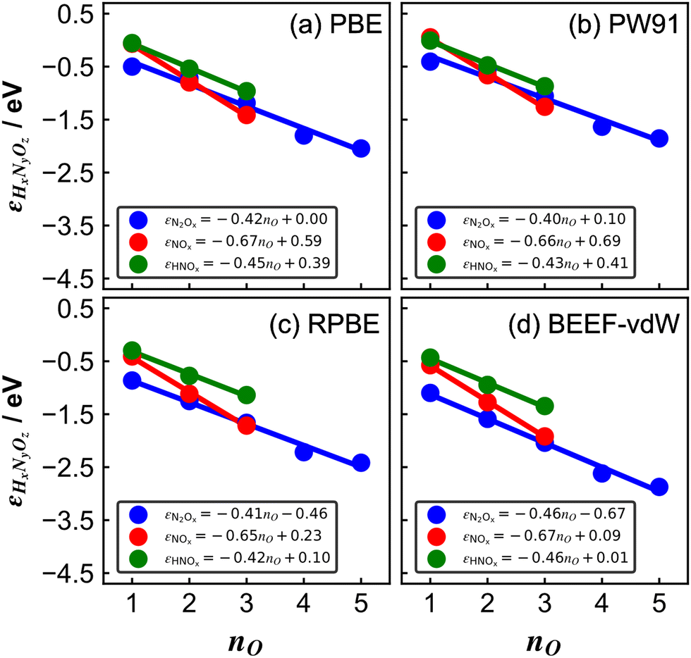 | ||
| Fig. 3 Errors of several nitrogen oxides as a function of the number of oxygen atoms in their structure for various xc-functionals: (a) PBE, (b) PW91, (c) RPBE, and (d) BEEF-vdW. In all panels, blue, red, and green are the trends of molecules with the general formulas N2Ox, NOx, and HNOx, respectively. The linear equation is reported in each case. Reproduced from ref. 29, licensed under CC BY 4.0 (https://creativecommons.org/licenses/by/4.0/). | ||
First, one can assume that the DFT errors of groups of atoms are equal to those encountered in analogous molecules, and then sequentially correct the errors of larger compounds (e.g., the molecule NO2 is analogous to the ONO backbone in HNO2 and HNO3 and, thus, their errors are assumed to be identical). In principle, the sequence progresses from simple (small) to complex (large) molecules. The flowchart of this procedure, referred to as “sequential”, is provided in Fig. 4, where each gray step deals with a specific group of atoms.
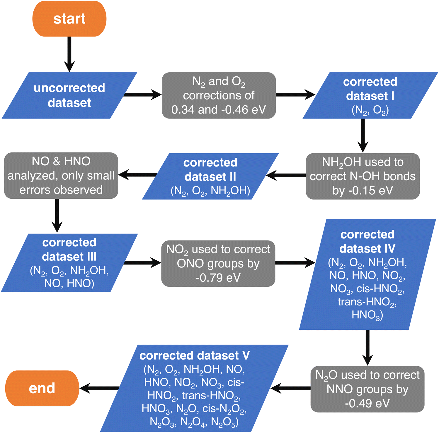 | ||
| Fig. 4 Flowchart of the chemically intuitive sequential method to detect the gas-phase errors of increasingly large molecules with N, O and H. Blue parallelograms represent the different sets of molecules and gray boxes represent the evaluation of specific errors in their thermochemical data. Reproduced from ref. 28, licensed under CC BY 4.0 (https://creativecommons.org/licenses/by/4.0/). | ||
Second, as shown in Table 2,28 a matrix representation of each molecule can serve as the basis to identify ill-described bonds within the molecules of the dataset. Once the structure of each molecule in the dataset is represented by the (single, double, triple) bonds between the atoms, an automatic optimization can be made using as free parameters the errors in the bonds. Along the lines of previous approaches,6,40 the MAE and MAX (or combinations thereof) with respect to experimental formation energies can be used as objective functions and minimized. In principle, this requires less human input than the method based on chemical intuition but leads to larger residual errors upon optimization. This procedure is referred to as automatic optimization 1 (AO1). For instance, HNO3(g) contains two N–O bonds and one NO bond, as shown in Fig. 5a.
| Species | Bonds | Groups of atoms | ||||||
|---|---|---|---|---|---|---|---|---|
| N–O | NO |
N–N | O–H | ONO | NNO | NOH | NN | |
| NH2OH | 1 | 0 | 0 | 1 | 0.0 | 0.0 | 1.0 | 0.0 |
| NO | 0 | 1 | 0 | 0 | 0.0 | 0.0 | 0.0 | 0.0 |
| HNO | 0 | 1 | 0 | 0 | 0.0 | 0.0 | 0.0 | 0.0 |
| NO2 | 1 | 1 | 0 | 0 | 1.0 | 0.0 | 0.0 | 0.0 |
| NO3 | 2 | 1 | 0 | 0 | 1.5 | 0.0 | 0.0 | 0.0 |
| trans-HNO2 | 1 | 1 | 0 | 1 | 0.5 | 0.0 | 1.0 | 0.0 |
| cis-HNO2 | 1 | 1 | 0 | 1 | 0.5 | 0.0 | 1.0 | 0.0 |
| HNO3 | 2 | 1 | 0 | 1 | 1.0 | 0.0 | 1.0 | 0.0 |
| N2O | 0 | 1 | 1 | 0 | 0.0 | 1.0 | 0.0 | 0.0 |
| cis-N2O2 | 0 | 2 | 1 | 0 | 0.0 | 2.0 | 0.0 | −1.0 |
| N2O3 | 1 | 2 | 1 | 0 | 1.0 | 1.0 | 0.0 | 0.0 |
| N2O4 | 2 | 2 | 1 | 0 | 2.0 | 0.0 | 0.0 | 1.0 |
| N2O5 | 4 | 2 | 0 | 0 | 2.0 | 0.0 | 2.0 | 0.0 |
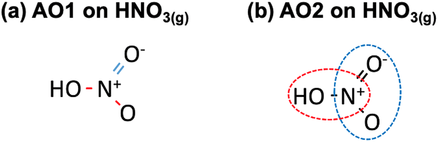 | ||
| Fig. 5 (a) Chemical bonds present in HNO3(g) as identified in AO1: N–O in red and NO in blue. (b) NOH (encircled in red) and ONO backbones (enclosed in blue) identified in HNO3(g) as per AO2. | ||
Third, the errors of the groups of atoms identified by means of the sequential approach are set as adjustable parameters in an optimization problem, see Table 2. Since there are several possibilities to represent the molecules, multiple representations may lead to different correction schemes with varying performance. In such cases, it is advisable to make an ensemble of representations and choose the one providing lower final errors. We refer to this procedure as automatic optimization 2 (AO2). Fig. 5b depicts how HNO3(g) can be decomposed into ONO and NOH groups.
Fig. 6 summarizes the performance of the (i) sequential, (ii) AO1, and (iii) AO2 approaches when used to correct the PBE-calculated Gibbs energies of the thirteen nitrogen compounds listed in Table 2. The MAE and MAX values before and after the corrections are shown for each method. Table 3 shows the problematic groups of atoms and/or bonds identified by each method with their respective errors. All the methods substantially decrease the large, uncorrected MAE (0.83 eV) and MAX (1.98 eV) obtained with plain PBE. Moreover, the three methods use the same number of variables: both AO2 and the sequential approach identified five problematic structures, and AO1 employs five different bonds to correct the errors in the Gibbs energies. AO2 yields the lowest errors (final MAE/MAX of 0.05/0.08 eV), followed by the sequential method, which resulted in a similar MAE of 0.07 eV but a larger MAX of 0.19 eV. Finally, AO1 produces the largest residual errors, with a MAE of 0.11 eV and a MAX of 0.26 eV.
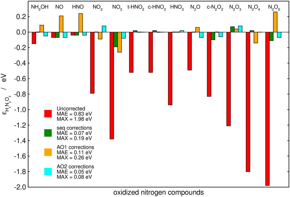 | ||
| Fig. 6 Initial and final errors in the PBE-calculated Gibbs energies of thirteen nitrogen compounds after being corrected by a chemically intuitive sequential approach (in green), an automated bond-based approach (AO1, in orange), and an automated version of the chemically intuitive, sequential approach (AO2, in cyan). Reproduced from ref. 28, licensed under CC BY 4.0 (https://creativecommons.org/licenses/by/4.0/). | ||
| Method | N–H | N–O | NO |
N–N | O–H | NOH | ONO | NNO |
|---|---|---|---|---|---|---|---|---|
| AO1 | 0.00 | −0.42 | −0.29 | −0.26 | 0.18 | — | — | — |
| AO2 | 0.00 | — | — | −0.07 | — | −0.09 | −0.87 | −0.42 |
| Sequential | 0.00 | — | — | −0.24 | — | −0.15 | −0.79 | −0.49 |
2.3 Anticipating error cancellation
Once estimated, the DFT errors of the molecules can be used to anticipate the degree of error cancellation in a chemical reaction. Granda-Marulanda et al.34 assessed the errors of CO2 and CO and noted a constant difference between them of ∼0.40 eV for various GGA functionals, see Fig. 7. Hence, DFT at the GGA level is unable to simultaneously provide an accurate description of both molecules and one cannot rely on error cancellation for several important catalytic reactions, such as CO2 electroreduction to CO and CO electrooxidation to CO2, and the water–gas shift and its reverse reaction in heterogeneous catalysis. Similarly, it has been shown that the error difference between the nitro and nitrite functional groups is also constant and no larger than ∼0.10 eV for different GGAs.25 In view of such moderate errors, for reactions between similar species or functional groups, such as the nitro-nitrite isomerization, error cancellation can be expected.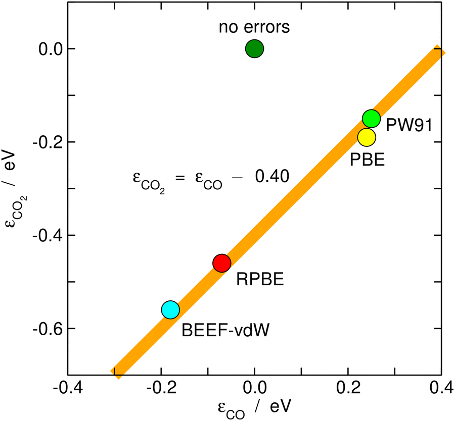 | ||
| Fig. 7 Correlation between the gas-phase errors in CO and CO2 for various xc-correlation functionals. The hypothetical perfect agreement between DFT and experimental values is marked in dark green. | ||
Before closing this section, we note that the aforementioned methods are based on different considerations and thus yield different types and number of errors, with varying numerical results. Depending on data availability and the nature of the intended calculations, one could be preferred over the others. However, as each approach is formulated differently, it is advisable to consistently use the same approach throughout a given study. Regardless of the scheme chosen, a detailed appraisal of gas-phase errors is advised at the early stages of any DFT-based electrocatalysis study for the reasons explained in the next sections. Furthermore, we emphasize that the values in Table 1 can be used to model any electrocatalytic reaction involving the species and functional groups therein, as long as the compounds are in the gas phase. Of course, the specific values of the errors do change from one xc-functional to another and may change when using different codes, pseudopotentials, or sets of calculation details.
3. Effects on thermodynamic properties
3.1 Reaction energies and equilibrium potentials
A variable of great interest in electrochemistry is the equilibrium potential (U0), which indicates the maximum voltage a spontaneous redox reaction can deliver or, conversely, the minimum voltage that must be supplied to drive a nonspontaneous redox reaction.59 Moreover, the equilibrium potential is necessary to calculate the thermodynamic overpotential, which is often used by CHE-based models as a metric for the catalytic activity of materials. In this order of ideas, the equilibrium potential is a reference point for the optimization and design of catalysts, both in theory and experiments.1,60–63For a reduction reaction, U0 is related to the reaction Gibbs energy (ΔrG) and the number of transferred electrons (n) by means of eqn (11).
| U0 = −ΔrG/n | (11) |
Table 4 compares the DFT-calculated Gibbs energies and equilibrium potentials with experiments for five reactions. The predictions of different xc-functionals are shown in each case. The last column shows that the errors (DFT minus experiments) in the equilibrium potential (εU0) are a fraction of the errors in the Gibbs energy (εΔrG). In fact, for the CO2 reduction to CH4 (last row), the substantial BEEF-vdW free-energy error of 0.81 eV yields an equilibrium potential error of only ∼100 mV. Again, we stress that small errors in equilibrium potentials are not necessarily indicative of agreement between DFT and experiments, and resorting to reaction energies is advisable.
| Reaction | xc-Functionala | DFT | Error | ||
|---|---|---|---|---|---|
| ΔrG | U 0 | ε ΔrG | ε U 0 | ||
| a The values for the unreferenced functionals were obtained in this work. b Calculations of NO3(aq)− are based on the DFT-energies reported in ref. 29 and experimental data36 following the approach in ref. 51. In all the cases, the differences between the integral of the specific heats of the products and reactants from 0 K to 298.15 K were neglected when computing the DFT free energies of reaction. | |||||
| (1) O2(g) + 2H+(aq) + 2e− → H2O2(aq) ΔrG = −1.36 U0 = 0.68 | PBE64 | −1.14 | 0.57 | 0.22 | −0.11 |
| RPBE64 | −0.90 | 0.45 | 0.46 | −0.23 | |
| BEEF-vdW64 | −0.88 | 0.44 | 0.48 | −0.24 | |
| SCAN64 | −1.10 | 0.55 | 0.26 | −0.13 | |
| TPSS64 | −0.92 | 0.46 | 0.44 | −0.22 | |
| PBE064 | −1.18 | 0.59 | 0.18 | −0.09 | |
| B3LYP64 | −1.12 | 0.56 | 0.24 | −0.12 | |
| (2) O2(g) + 4H+(aq) + 4e− → 2H2O(l) ΔrG = −4.92 U0 = 1.23 | PBE26 | −4.46 | 1.11 | 0.46 | −0.12 |
| RPBE26 | −4.18 | 1.04 | 0.74 | −0.19 | |
| BEEF-vdW26 | −4.11 | 1.03 | 0.81 | −0.20 | |
| SCAN | −4.45 | 1.11 | 0.47 | −0.12 | |
| TPSS | −4.06 | 1.01 | 0.86 | −0.22 | |
| PBE0 | −4.68 | 1.17 | 0.24 | −0.06 | |
| B3LYP | −4.57 | 1.14 | 0.35 | −0.09 | |
| (3) N2(g) + 6H+(aq) + 6e− → 2NH3(g) ΔrG = −0.34 U0 = 0.06 | PBE29 | −0.68 | 0.11 | −0.34 | 0.06 |
| RPBE29 | −0.31 | 0.05 | 0.03 | 0.00 | |
| BEEF-vdW29 | −0.03 | 0.01 | 0.31 | −0.05 | |
| SCAN | −0.67 | 0.11 | −0.33 | 0.05 | |
| TPSS29 | −0.19 | 0.03 | 0.15 | −0.02 | |
| PBE029 | −0.91 | 0.15 | −0.57 | 0.09 | |
| B3LYP29 | −0.48 | 0.08 | −0.14 | 0.02 | |
| (4) CO2(g) + 8H+(aq) + 8e− → CH4(g) + 2H2O(g) ΔrG = −1.17 U0 = 0.15 | PBE34 | −0.97 | 0.12 | 0.20 | −0.03 |
| RPBE34 | −0.65 | 0.08 | 0.52 | −0.07 | |
| BEEF-vdW34 | −0.36 | 0.05 | 0.81 | −0.10 | |
| SCAN | −1.08 | 0.14 | 0.09 | −0.01 | |
| TPSS | −0.59 | 0.07 | 0.58 | −0.07 | |
| PBE0 | −1.37 | 0.17 | −0.20 | 0.02 | |
| B3LYP | −1.01 | 0.13 | 0.16 | −0.02 | |
| (5)b 2NO3−(aq) + 12H+(aq) + 10e− → N2(g) + 6H2O(l) ΔrG = −12.44 U0 = 1.24 | PBE | −10.22 | 1.02 | 2.22 | −0.22 |
| RPBE | −10.26 | 1.03 | 2.17 | −0.22 | |
| BEEF-vdW | −10.10 | 1.01 | 2.34 | −0.23 | |
| SCAN | −10.95 | 1.10 | 1.48 | −0.15 | |
| TPSS | −10.08 | 1.01 | 2.36 | −0.24 | |
| PBE0 | −11.51 | 1.15 | 0.93 | −0.09 | |
| B3LYP | −11.79 | 1.18 | 0.64 | −0.06 | |
The results in Tables 1 and 4 indicate that some xc-functionals provide outstanding results for certain molecules and reactions while performing poorly in other cases. For instance, RPBE displays the lowest errors in ΔrG of the ammonia synthesis reaction (0.03 eV and an error in U0 of −0.01 V) but displays errors above 0.45 eV for reactions involving oxygen-containing compounds. Similarly, PBE0 outperforms GGA and meta-GGA functionals in nearly all cases except the ammonia synthesis reaction, where it yields the worst prediction (an error of 0.57 eV). That said, some overall conclusions can be extracted: in general, the MAEs of GGA/meta-GGA functionals are similar for reactions (1)–(4) in Table 4 (0.39/0.35 eV, 0.67/0.67 eV, 0.23/0.24 eV, and 0.51/0.34 eV, respectively) and so are the MAXs (0.48/0.44 eV, 0.81/0.86 eV, 0.33/0.34 eV, and 0.81/0.58 eV). Except for the ammonia synthesis reaction, hybrids perform better than GGA and meta-GGA functionals, producing the lowest MAEs and MAXs for the reactions in Table 4 (reaction 1: MAE = 0.21, MAX = 0.24 eV; reaction 2: MAE = 0.29, MAX = 0.35 eV; reaction 4: MAE = 0.18, MAX = 0.20 eV; reaction 5: MAE = 0.79, MAX = 0.93 eV), with B3LYP generally providing the lowest errors. Nevertheless, all these results show that while some functionals perform better than others, the specific errors are generally not small enough to yield accurate predictions (e.g., MAE/MAX values below 0.10 eV). For instance, the errors of B3LYP for reaction 5 are >0.30 eV in Table 4. We note that once the errors are corrected, the experimental results are mimicked by all functionals. Therefore, in general, gas-phase corrections are advisable regardless of the xc-functional used.
Error analyses can also be extended to reactions where solvated and liquid compounds are involved. For aqueous compounds, the DFT energies of gas-phase references are combined with experimental data to circumvent the DFT modelling of liquids, which is arduous.1,65–68 A clear example is the DFT modelling of nitrate (NO3(aq)−) from gaseous HNO3.51 In this case, the free energy of gaseous HNO3, easily obtained from DFT, is combined with the experimental vaporization (0.075 eV) and solution free energies (0.317 eV) to indirectly obtain the free energy of NO3(aq)−,36 as shown in Fig. 8. This semiempirical energy can then be used to calculate the equilibrium potential of nitrate reduction reactions. Given that the error in the DFT-calculated free energy of HNO3 is larger than 1 eV for several GGA and meta-GGA xc-functionals,25,28,29,51 overlooking it leads to seriously impaired reaction energies and equilibrium potentials, especially for reactions with small number of transferred electrons.
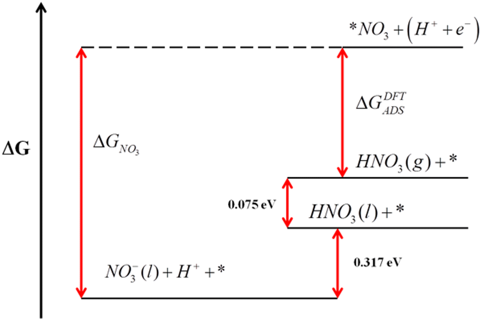 | ||
| Fig. 8 Gibbs energy scale for HNO3 relating the free energies of different states. Reproduced from ref. 51 Copyright 2013, Royal Society of Chemistry. | ||
3.2 Adsorption and desorption energies
When modelling electrocatalytic reactions, adsorption and desorption steps occur at least once and are, therefore, central in the analysis. The adsorption of species A on a free surface site (*) can be represented as follows:| A + * → *A | (12) |
| ΔGADSA = G*A − G* − GA | (13) |
Besides, gas-phase errors might modify the adsorption/desorption energies such that intermediate adsorption/desorption steps become (or cease to be) limiting in a reaction. In principle, when the binding is considerably modified by gas-phase corrections, opposing strategies to optimize a given catalyst may be obtained before and after the corrections. Consider the coupling reaction A(g) + B(g) → AB(g), with εAB representing the DFT gas-phase error of AB(g). Fig. 9 shows the adsorption of A and B, their surface coupling, and the desorption of AB. The inset shows a schematic bar plot for the desorption Gibbs energy of AB(g) when the gas-phase errors are not considered and when they are accounted for, the difference being εAB, following eqn (4). Catalyst deactivation by site blocking is likely to be observed if the magnitude of the correction term εAB is such that the corrected desorption energy is larger than 0.75 eV, which is an accepted threshold for viable kinetics at room temperature.69,70 However, this deactivation would not be predicted by the uncorrected results. Further examples are provided in the next sections.
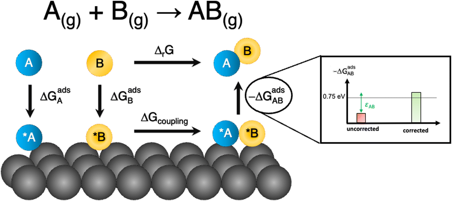 | ||
| Fig. 9 Scheme of a catalytic coupling reaction. Inset: Desorption energy of AB before (in red) and after (in green) correcting gas-phase errors. In the example, without gas-phase errors, easy desorption is predicted, whereas site blocking is predicted upon incorporating them. Adapted from ref. 25 Copyright 2021, John Wiley and Sons. | ||
4. Implications for free-energy diagrams
4.1 Free-energy diagrams
DFT allows us to estimate, within a reasonable timeframe, the energies of adsorbed intermediates, which is something usually not attainable in experiments, in particular for short-lived species. From the Gibbs energies of the intermediates and the CHE model,1 it is possible to build free-energy diagrams for entire electrochemical reaction networks. These diagrams are used (i) to establish the feasibility of a given reaction pathway at different applied potentials and pH, and (ii) to quantify the catalytic performance of several materials through the identification of the potential-limiting step and the calculation of the overpotential. In fact, free-energy diagrams are arguably the most widespread activity plots in electrocatalysis.1,6,9,10,71As mentioned before, if an electrocatalytic reaction involves gas-phase compounds, the DFT errors will affect the equilibrium potentials, which distorts the free-energy diagrams of ideal catalysts. For the 4-electron O2 reduction and evolution reactions on the ideal catalyst (Table 4),26 the errors in O2 (εO2) are usually above 0.30 eV for several functionals. These errors are not only detrimental to the calculation of the equilibrium potential but also to the energetics of individual reaction steps, preventing the accurate estimation of limiting steps. For instance, the reaction energy for oxygen reduction calculated with RPBE is −4.18 eV, according to Table 4. This means that RPBE predicts that oxygen reduction is not as exothermic as it should (by more than 0.70 eV) and, as a result, the equilibrium potential is as low as 1.04 V vs. RHE. This corresponds to an error of around 200 mV.
Similarly, the oxygen reduction reaction to hydrogen peroxide on the ideal catalyst using several xc-functionals was studied recently (Table 4).27 This reaction involves the errors in molecular oxygen and hydrogen peroxide, εO2 and εH2O2, which are large and different for GGA, GGA-vdW, meta-GGA, and hybrid xc-functionals.27 In Fig. 10a, the free-energy diagram for H2O2 production at 0 V vs. RHE without gas-phase corrections is shown. Fig. 10b shows the diagram with gas-phase corrections applied only to O2. In both cases, the ideal catalyst predicted using experimental data is shown in black. Only when both εO2 and εH2O2 are corrected can DFT mimic experiments.
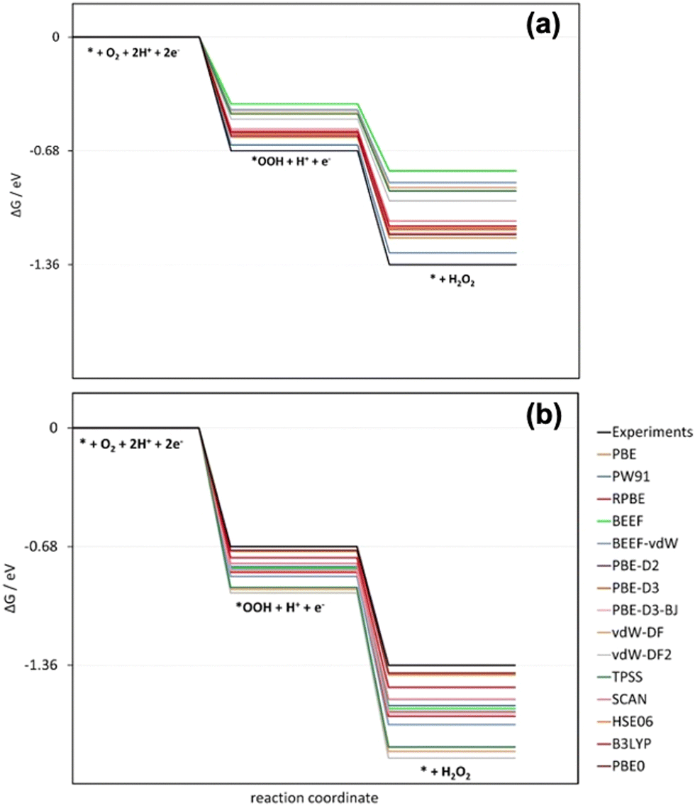 | ||
| Fig. 10 Free-energy diagrams at 0 V vs. RHE for hydrogen peroxide production on the ideal catalyst using several xc-functionals. (a) Gas-phase corrections are not included. (b) Only the errors in O2 are corrected. In black in both panels is the experimentally expected profile, obtained when both errors are corrected. Reproduced from ref. 27, licensed under CC BY 4.0 (https://creativecommons.org/licenses/by/4.0/). | ||
Furthermore, Fig. 10a shows that before O2 and H2O2 are corrected, DFT at different rungs of Jacob's ladder underestimates the reaction energy and the equilibrium potential. As a result, the free-energy diagram of the ideal catalyst deviates considerably from what can be expected from experiments. Once the O2 error is corrected, DFT gives more negative estimates of all the energies. The switch is introduced by εH2O2, which is negative for all the DFT functionals scrutinized, see Table 1.
| ΔrG(U) = ΔrG° + eU | (14) |
Limiting potentials may sometimes be affected by gas-phase errors, and free-energy diagrams are suitable tools to visualize and rationalize such effects. In fact, the influence of εCO2 and εCO has been shown on CO2 reduction to CO on Au electrodes,34 and close agreement with experiments is reached if these errors are corrected. Fig. 11 shows the PBE-calculated free-energy diagrams of CO2 reduction to CO following the standard pathway via *COOH and *CO,74 with uncorrected and corrected Gibbs energies. For Au(111) electrodes, the first hydrogenation is the potential-limiting step, and the energy decreases from 0.90 to 0.71 eV once the CO2 Gibbs energy is corrected by −0.19 eV, which is the PBE error for CO2 (Table 1).34 Accordingly, the onset potential changes from −0.90 to −0.71 V vs. RHE, compared to the experimental onset potential of −0.66 V vs. RHE,75 so the difference with respect to experiments is reduced from 0.24 to 0.05 V once the gas-phase errors are corrected. This analysis was made for numerous metal electrodes and the calculated onset potentials were found to approach the experimental ones upon correcting the DFT errors, see Fig. 12.
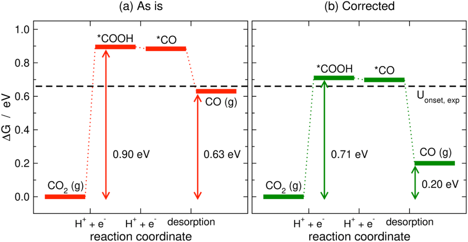 | ||
| Fig. 11 PBE-calculated free-energy diagrams of the CO2RR to CO on Au(111) without (a) and with (b) gas-phase corrections. The Gibbs energies corresponding to the onset and equilibrium potentials are shown in each case along with the experimental onset potential (dashed line). Reproduced from ref. 34, licensed under CC-BY-NC-ND (https://creativecommons.org/licenses/by-nc-nd/4.0/). | ||
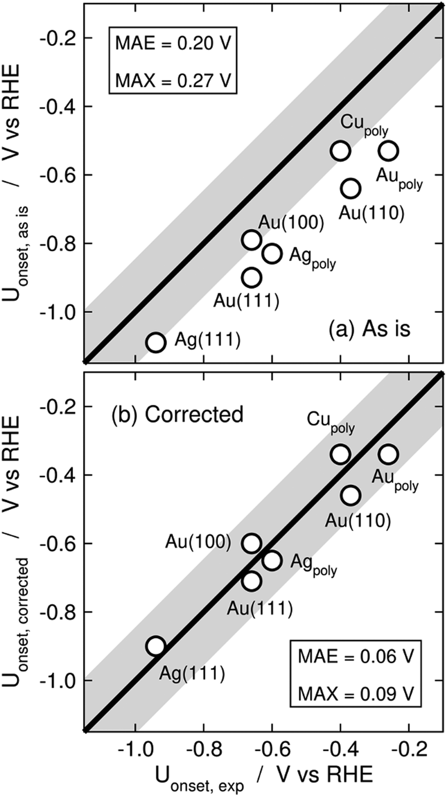 | ||
| Fig. 12 Parity plots for the PBE-calculated and experimental onset potentials of CO2 reduction to CO on metal electrodes (a) without and (b) with gas-phase corrections. The MAE and MAX are reported in each case. The gray band around the parity line has a vertical width of 0.2 V. Reproduced from ref. 34, licensed under CC-BY-NC-ND (https://creativecommons.org/licenses/by-nc-nd/4.0/). | ||
We note in passing that free-energy diagrams also show the effects of the gas-phase errors on the reaction energy (and thus on the equilibrium potential), which were previously assessed through eqn (11) in Section 3. In Fig. 11, the reaction energy goes from 0.63 to 0.20 eV, which is the experimental value.69
Finally, free-energy diagrams are also affected when intermediate desorption takes place within an electrocatalytic reaction. This can lead to different strategies to optimize a given catalyst, as exemplified in Fig. 13 for the hypothetical electrocatalytic reduction of AB(g) to AH2(g) and BH2(g), in which four proton–electron transfers take place: AB(g) + 4 (H+ + e−) → AH2(g) + BH2(g). In this reaction, it is assumed that either (i) AB(g) and AH2(g) are properly described by DFT (εAB ≈ εAH2 ≈ 0) or (ii) have already been corrected, which makes BH2(g) the only source of errors. Fig. 13 presents the free-energy diagram of the reaction, considering the energy level of the intermediate desorption of BH2(g) with and without gas-phase corrections. Without corrections, the potential-limiting step (PLSunc) is the desorption of BH2(g) (second proton–electron transfer). After correcting the gas-phase error, the energy of the desorption step decreases by as much as the error in BH2(g) (εBH2) such that the first proton–electron transfer is the actual potential-limiting step (PLScorr). The inset of Fig. 13 depicts how the potential of the second hydrogenation is modified by including the gas-phase correction compared to the energy of the first hydrogenation step. Thence, *AB → *ABH should guide the optimization of the catalyst instead of *ABH → *A + BH2(g).
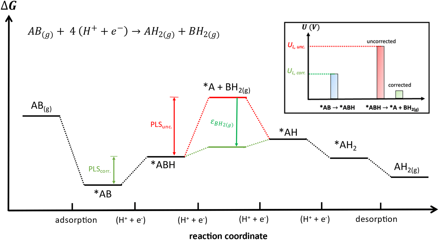 | ||
| Fig. 13 Free-energy diagram of the hypothetical electrocatalytic reduction of AB(g) to AH2(g) and BH2(g). The Gibbs energies without and with gas-phase corrections for BH2 are shown in red and green, respectively. PLS: potential-limiting step, which switches from the second (PLSunc) to the first hydrogenation step (PLScorr) after applying the corrections. Inset: Potential of the second hydrogenation before (red) and after (green) the corrections compared to that of the first hydrogenation (blue). | ||
5. Scaling relations and volcano plots
5.1 Scaling relations
When two sets of adsorption energies on various materials are plotted against each other, a linear relationship may emerge, especially when the adsorbates bear some similarities.76–82 Adsorption-energy scaling relations reveal linear connections between the intermediates of electrocatalytic reactions and enable the making of systematic, trend-based studies to understand the working principle of catalysts and design enhanced active sites.1,5,11,74 In addition, there are linear relationships between adsorption energies and thermochemical, structural and electronic features of materials, which have been widely used for catalyst screening and design.83–85Fig. 14a displays linear relations between the adsorption energies of different atoms (C and Si, N and P, O and S, F and Cl) on top sites of near-surface alloys of Pt(111) and transition metals while Fig. 14b and c show examples of two different sets of adsorption-energy scaling relations: (i) adsorption energies as a function of a structural descriptor, namely the generalized coordination number ( ),86–88 and (ii) the adsorption energies of *OOH, *O and *OH as functions of the energies of formation of bulk metal oxides (MO), LaMO3 perovskites, and SrMO3 perovskites (M: metals between Ti and Cu).
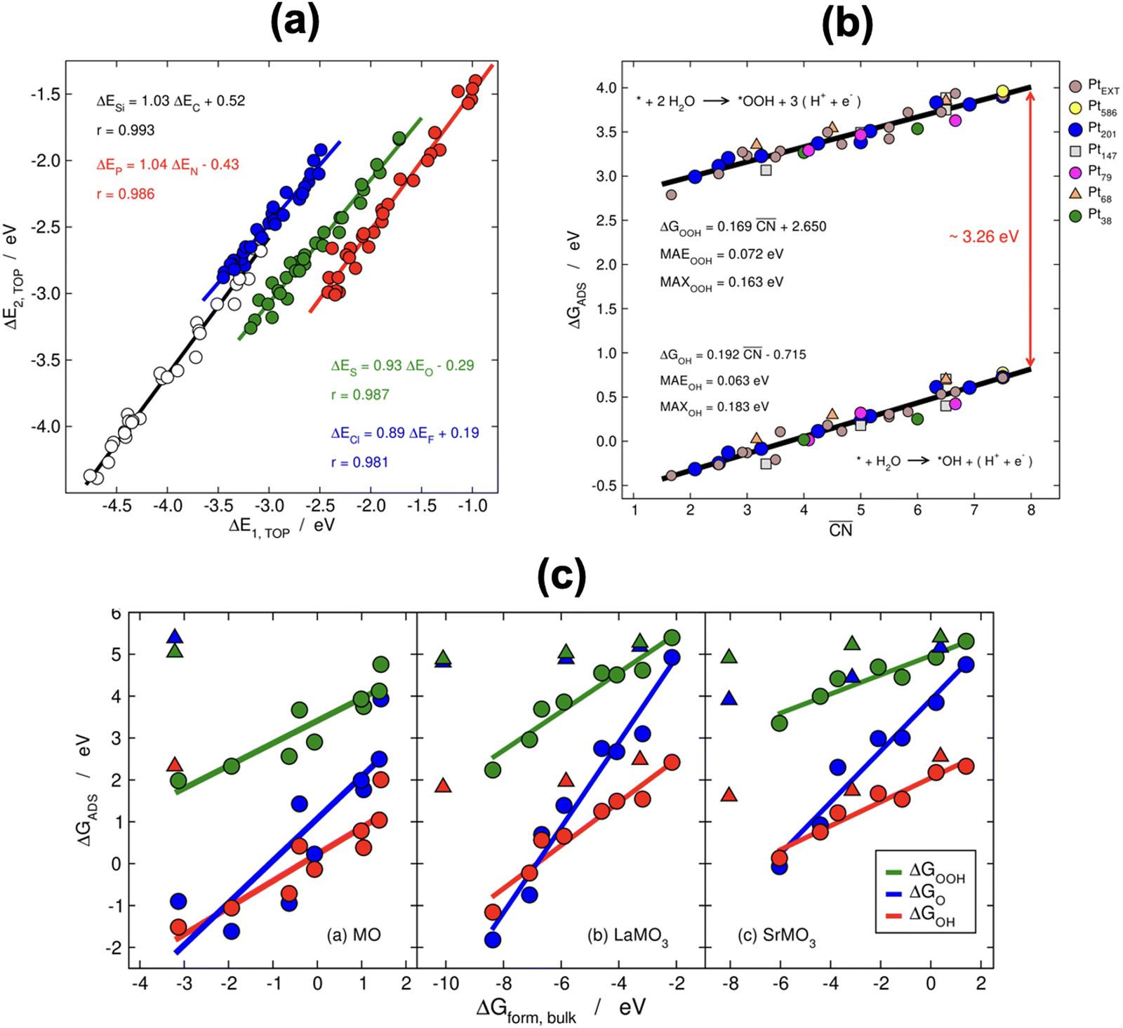 | ||
Fig. 14 (a) Scaling relations between the adsorption energies of different atoms (C, Si, N, P, O, S, F, Cl) on top sites of near-surface alloys of Pt(111) and transition metals. Reproduced with permission from ref. 78 Copyright 2012, American Physical Society. (b) Adsorption energies of *OOH and *OH on different sites at platinum nanoparticles and extended surfaces as a function of the generalized coordination number ( ). Reproduced with permission from ref. 87 Copyright 2017, AAAS. (c) Correlations between the adsorption energies of *OOH, *O, and *OH and the formation energy of bulk MO, LaMO3, and SrMO3, where M is a metal from Ti to Cu. Triangles are data for which the linear relationships do not apply. Reprinted (adapted) with permission from ref. 84 Copyright 2014, American Chemical Society. ). Reproduced with permission from ref. 87 Copyright 2017, AAAS. (c) Correlations between the adsorption energies of *OOH, *O, and *OH and the formation energy of bulk MO, LaMO3, and SrMO3, where M is a metal from Ti to Cu. Triangles are data for which the linear relationships do not apply. Reprinted (adapted) with permission from ref. 84 Copyright 2014, American Chemical Society. | ||
As discussed in Section 3, DFT gas-phase errors influence adsorption energies. Therefore, gas-phase errors affect adsorption-energy scaling relations. Because the errors are constant for a given xc-functional and a fixed pair of adsorbates, the offsets of scaling relations are modified but the slopes remain unchanged. This is shown in Fig. 15 for the scaling relations between the RPBE-calculated adsorption energies of *NO3, *NO2, and *NO on a series of metalloporphyrins with different transition-metal centers. Since *NO3, *NO2, and *NO have sizable gas-phase errors (−1.72, −1.12, and −0.41 eV, respectively), each data point in Fig. 15 is displaced along the direction of the εT vector (in brown) once the energies are corrected. The corresponding abscissa component of εT is the nitric oxide error, εNO, whereas the ordinate components correspond to εNO3 and εNO2 in panels a and b, respectively. For example, in the plot of ΔGNO3vs. ΔGNO the uncorrected intercept is 0.47 eV and the slope is 1.76. Given that εNO3 = −1.72 eV and εNO = −0.41 eV, the corrected intercept is 0.47 − 1.72 + 1.76 × 0.41 = −0.52 eV.
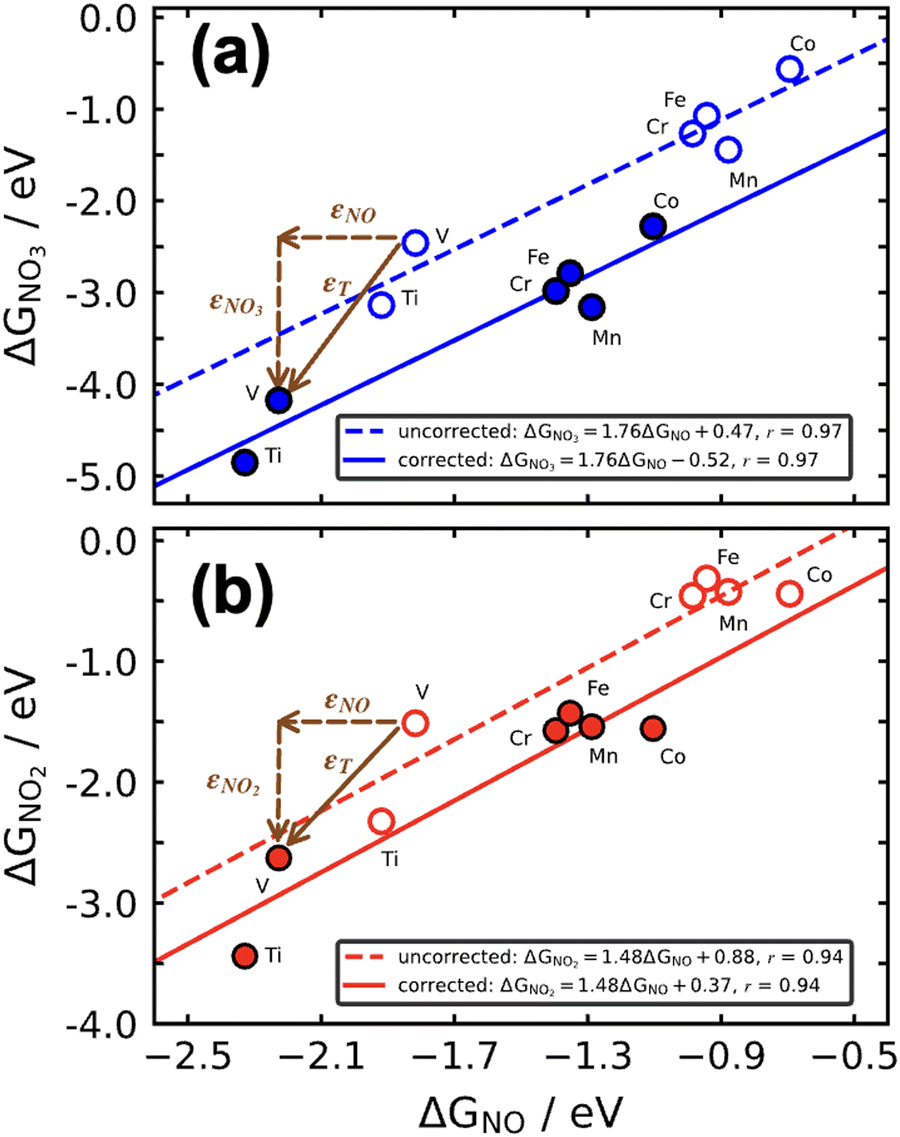 | ||
| Fig. 15 Free energies of adsorption of *NO3 (a) and *NO2 (b) versus that of *NO on metalloporphyrins. Dashed lines and open circles correspond to uncorrected energies, solid lines and solid circles correspond to energies upon gas-phase corrections. Brown vectors on the V-containing porphyrin show the displacements introduced by the respective gas-phase errors. Reproduced from ref. 29, licensed under CC BY 4.0 (https://creativecommons.org/licenses/by/4.0/). | ||
We note in passing that while scaling relations are conventionally defined for the adsorption energies of two species on several materials calculated with a fixed computational setup, it is also possible to define them for two species on a given material calculated with various computational setups. Such scaling relations can help detect systematic anomalies in adsorption energies, as illustrated for RuO2 and *O, *OH and *OOH, for which an anomaly in the adsorption energy of *O was exposed that explains the incorrect activity prediction for oxygen evolution provided by the CHE for this material.39,89,90
5.2 Volcano plots
Scaling relations can be used to build Sabatier-type volcano plots, which are extensively used to display the trends in electrocatalytic activity of materials as a function of a given descriptor or a combination of them.1,11,71,88,91,92 These plots also establish the conditions for optimal catalysis, found at the top of the volcano, and have led to the discovery of promising electrocatalysts for important reactions.2,76,92,93If a metric for the catalytic activity is plotted against the energy of a key intermediate, bidimensional volcanoes are obtained. If the activity is plotted as a function of two or more intermediates, multidimensional volcanoes appear. An example of a bidimensional volcano plot is that of the oxygen evolution reaction on a variety of materials, shown in Fig. 16a. In turn, Fig. 16b is a contour plot relating the binding energies of *OH and *C2O2 with the activity for CO electroreduction to ethanol on different metals.
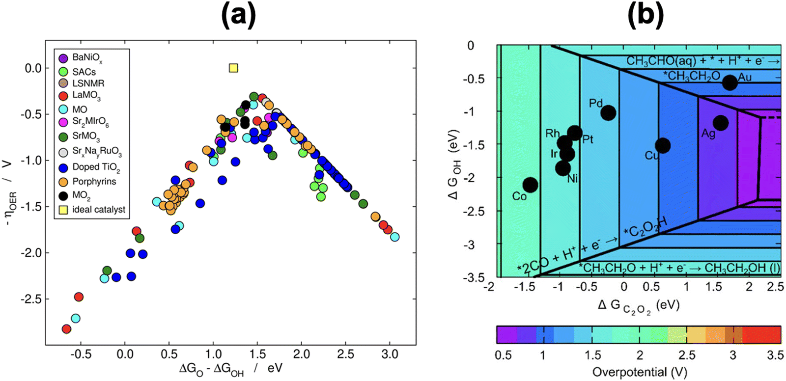 | ||
| Fig. 16 (a) Volcano plot for oxygen evolution on different materials. Reproduced from ref. 94, licensed under CC-BY 3.0 (https://creativecommons.org/licenses/by/3.0/). (b) Contour plot for CO reduction to ethanol on the (100) facet of different transition metals. In both panels, the overpotential is used as a metric for the catalytic activity. Reprinted (adapted) with permission from ref. 95 Copyright 2018, American Chemical Society. | ||
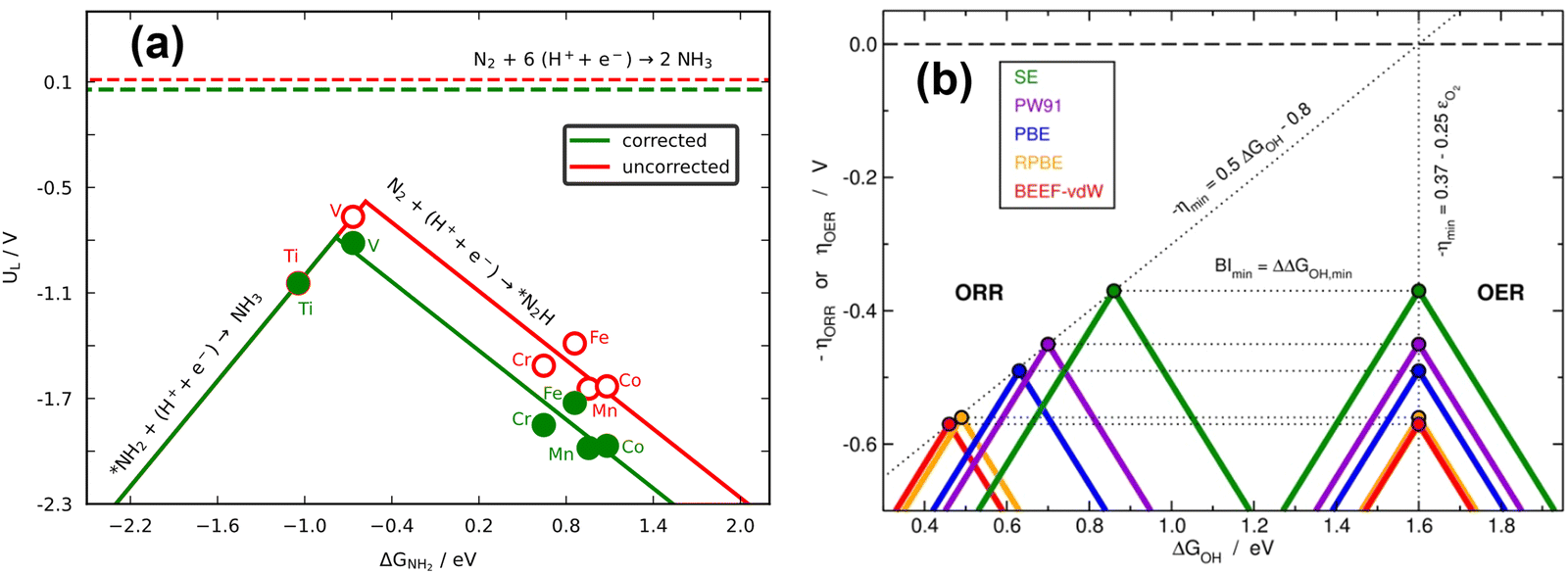
Because scaling relations are modified by gas-phase errors, it is expectable that volcano plots will also be affected by them. The effects depend on whether the limiting steps involve a gas-phase compound, as discussed below. First, let us consider the volcano plot in Fig. 17a for the ASR on metalloporphyrins using the PBE functional and ΔGNH2 (* + NH3 → *NH2 + H+ + e−, with NH3 assumed to be well-described by DFT,49 see Section 2, approach iv) as an activity descriptor. In this volcano, UL refers to the potential of the limiting reactions and is calculated as UL = −ΔGL/n, where ΔGL is the energy of the potential-limiting step in eV and n is the number of electrons transferred (typically 1 for an electrochemical step). Hence, if ΔGL involves gaseous compounds the errors of which are not corrected, it will yield an uncorrected UL (red volcano). If the gas-phase errors are taken care of, a corrected UL will be obtained (green volcano). The right leg of the volcano is usually limited by the hydrogenation of N2, which has a sizable gas-phase error (Table 1), while the left leg is limited by the hydrogenation of adsorbed *NH2 to produce NH3.96,97 The reaction on the left leg is not modified by the corrections because NH3 is thought to be well described by DFT. It is observed in Fig. 17a that upon correcting the errors, the volcano is not symmetrically reshaped, and the impact of that in catalysis is presented in Fig. 18a.
 | ||
| Fig. 17 (a) Volcano plot for electrochemical ammonia synthesis on different metalloporphyrins. In red: PBE results with no gas-phase corrections. In green: corrected PBE results. The dashed lines represent the equilibrium potentials. Reproduced from ref. 29, licensed under CC BY 4.0 (https://creativecommons.org/licenses/by/4.0/). (b) Volcanoes obtained with four GGAs for the OER and ORR. After accounting for all the gas-phase errors, a single semiempirical volcano (in green, SE) is obtained for each reaction. BI: bifunctional index for the ORR/OER redox performance. Reproduced from ref. 42, licensed under CC BY-NC-ND 4.0 (https://creativecommons.org/licenses/by-nc-nd/4.0/). | ||
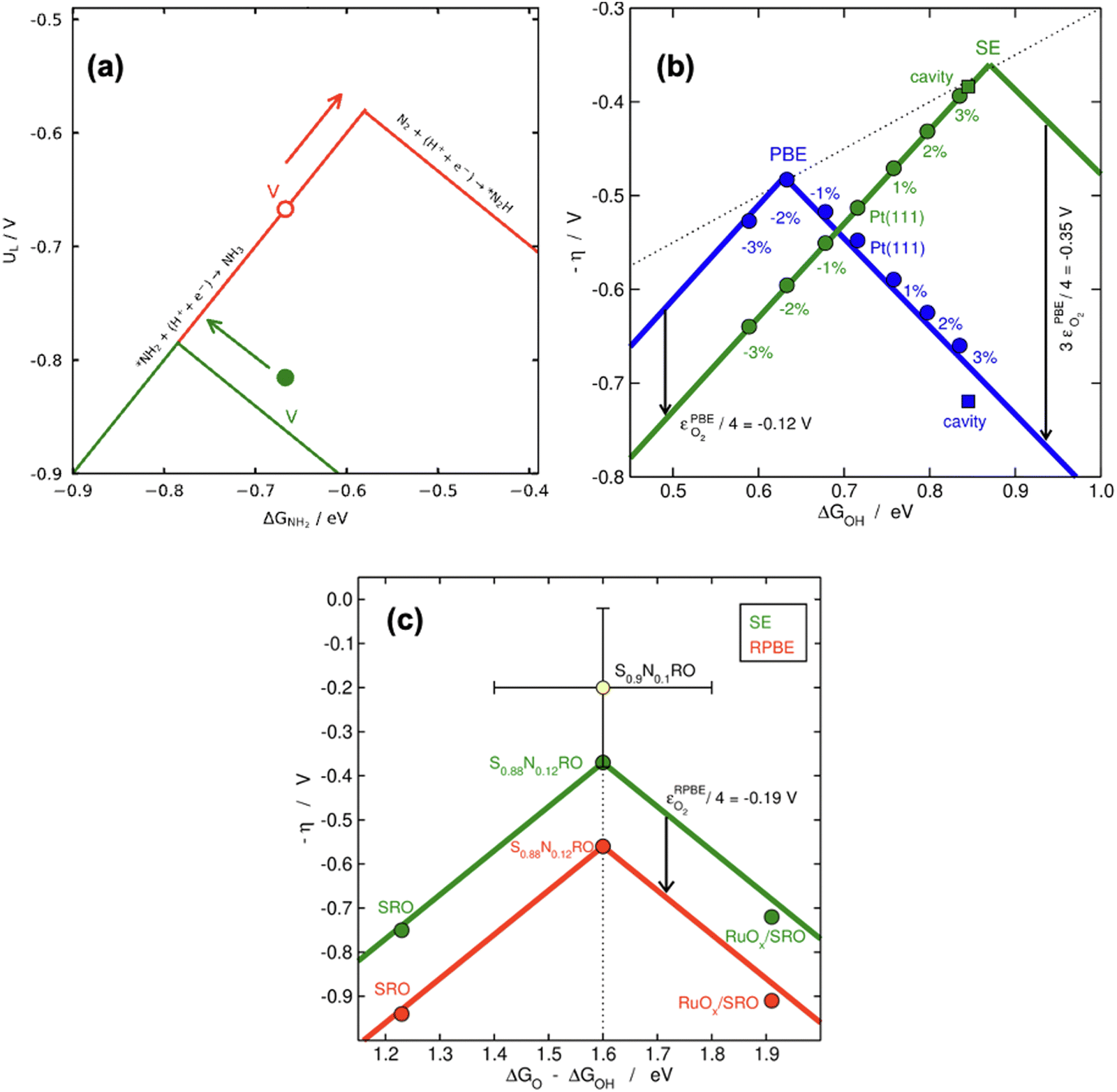 | ||
| Fig. 18 (a) Location of V-porphyrin before (in red) and after (in green) correcting the gas-phase errors in electrochemical ammonia synthesis. The arrows show the respective directions towards the top of the volcano. Reproduced from ref. 29, licensed under CC BY 4.0 (https://creativecommons.org/licenses/by/4.0/). (b) Effect of compressive/stretching strain and cavities on the catalytic activity of Pt(111) for the ORR with (green) and without (blue) gas-phase corrections. (c) Vertical offsetting of the OER volcano introduced by the error in O2. In yellow, an experimental datapoint which is only matched after the gaseous errors are semiempirically corrected. Panels b and c are reproduced from ref. 42, licensed under CC BY-NC-ND 4.0 (https://creativecommons.org/licenses/by-nc-nd/4.0/). | ||
According to recent work,42 knowledge of the potential-limiting steps suffices to analytically predict the effect of gas-phase errors on volcano plots. This is shown in Fig. 17b for the OER and ORR, which involve the error in O2, using four GGA functionals (PBE, PW91, RPBE, and BEEF-vdW).42 In this figure, the y-axis contains the ORR and OER overpotentials, which are defined with respect to the equilibrium potential as ηORR = U0ORR − UL,ORR and ηOER = UL,OER − U0OER (and U0ORR = U0OER). While the use of overpotentials is customary for ORR and OER modelling, UL is more used for other reactions. Fig. 17b illustrates one of the downsides of using overpotentials instead of potentials: overpotentials introduce the gas-phase errors of the overall reaction into the activity.
For the OER, the optimal adsorption energy of *OH used as descriptor (ΔGOH, calculated as the free energy of * + H2O → *OH + H+ + e− with water thought to be well described by DFT)49 does not change across functionals but the lowest overpotential, i.e., the top of the volcano, does change. This stems from the OER being typically limited by reaction steps in which no gas-phase errors are involved (*OH → *O + H+ + e− and *O + H2O → *OOH + H+ + e−). In striking contrast, both the lowest overpotential and the optimal ΔGOH change depending on the xc-functional for the ORR. This is because one of the potential-limiting steps involves molecular oxygen (* + O2 + H+ + e− → *OOH), which has usually large errors for several functionals. In view of that, the uncorrected ORR volcanoes in Fig. 17b are located to the left and below the corrected volcano. After corrections, the volcanoes of all the xc-functionals turn into the semiempirical one (denoted as SE) as the gas-phase errors are defined with respect to the corresponding experimental values (see eqn (3), εT = ΔrGDFT − ΔrGexp = ΔrHDFT − ΔrHexp). Lastly, the equations in Fig. 17b show that the location of the ORR and OER volcano apices can be analytically predicted on the basis of the error in O2 for all functionals following simple considerations. Full details can be found in ref. 42.
In principle, the descriptor of a volcano plot may help establish guidelines toward enhanced electrocatalysis. In other words, if the value of the descriptor that corresponds to the top of the volcano is reachable by means of some electronic or structural procedure, rational catalyst design is enabled.87 Gas-phase errors affect this process, as they mislocate the top of the volcano and alter the activity trends. This is shown for the ASR modelled with PBE in Fig. 18a.29 Without gas-phase corrections, the strategy to reach the top of the volcano is the opposite as when they are included: the uncorrected volcano prescribes the weakening of the adsorption energy of *NH2 on the V-porphyrin, whereas the corrected volcano suggests to strengthen it.
Similarly, Fig. 18b illustrates how the PBE errors in O2 modify the optimization strategy for the ORR: the uncorrected volcano (in green) displays low activity of cavities and suggests that stretching strain between −1% and −2% with respect to bulk Pt increases the catalytic activity of pristine Pt(111). Notwithstanding, after correcting the gas-phase errors, compressive strain is predicted to increase the catalytic activity with respect to Pt(111), and small cavities on Pt(111) are closest to the top. In this case, only the corrected volcano plot is in accordance with experiments, which have consistently shown that compressive strain and cavities enhance the activity of Pt(111) electrodes.87,98–101
Finally, there are cases in which the symmetric shift of a volcano might take place with concurrent effects on DFT predictions. This is the case for the RPBE-calculated OER volcano on different SrRuO3 electrodes (pristine SrRuO3, Na-doped SrRuO3, and RuOx layers on SrRuO3), as exemplified in Fig. 18c. For this reaction, the potential-limiting steps do not include O2, but the minimum overpotential (the difference between the equilibrium potential and the potential at the top of the volcano) involves εO2. This means that although the abscissa of the top remains unchanged (at 1.6 eV), εO2 shifts the volcano vertically, leading to larger overpotentials compared to ∼0.37 V, the value of the corrected model.10,42,61 Moreover, only after accounting for the gas-phase errors does the RPBE prediction agree with the experimental datapoint (in yellow) added to the plot on the basis of a semiempirical method.4,102
6. Summary and outlook
In the previous sections, DFT gas-phase errors were shown to exist at various levels of Jacob's ladder of xc-functionals for numerous molecules. Furthermore, the DFT error (εi) in the ground-state energy of a gaseous substance or in a set of gaseous compounds (denoted EDFTi), spreads through customary computational models used in heterogenous (electro)catalysis, preventing an accurate estimation of paramount quantities such as equilibrium potentials and free energies. In the light of all this, gas-phase errors may mislead the design of active and selective catalysts and/or result in models that only agree with experiments qualitatively, or that agree quantitatively only because of error cancellation.To summarize all this, Fig. 19 shows the origin, propagation, and spread of gas-phase errors, εi, through computational (electro)catalysis models. The black steps in Fig. 19 represent operations performed on the input datasets, which are depicted in blue. In Fig. 19 we differentiate between linear error spread and exponential error spread: the former is typical of thermodynamic models (yellow box) while the latter is typical of models in which reaction rates are calculated (red box).
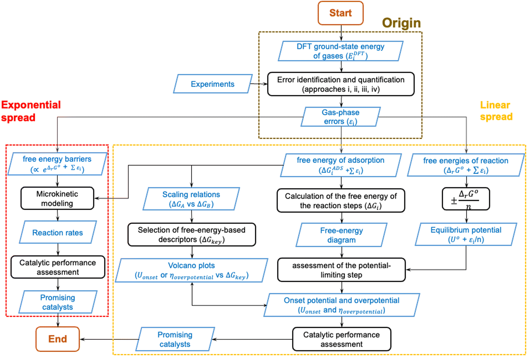 | ||
| Fig. 19 Schematics of gas-phase errors (εi) and their impact on electrocatalysis models. The origin (brown box), exponential spread (red box), and linear spread (yellow box) in computational (electro)catalysis models are shown. Black steps represent operations performed on different datasets, depicted as blue parallelograms. Data in the blue parallelograms might lead to erroneous quantities if the errors from “Origin” are not corrected. | ||
A particular example of the spread in the yellow box is found in Fig. 11 and 12, which come from the work of Granda-Marulanda et al.34 together with suitable experimental results75,103–105 on CO2(g) reduction to CO(g) on metal electrodes: when modelling this reaction, the uncorrected gas-phase energies lead to a reaction energy of 0.63 eV, which deviates significantly from the experimental value of 0.20 eV (Fig. 11).69 This wrongful reaction energy yields an equilibrium potential of −0.32 V vs. RHE which substantially departs from the experimental value of −0.10 V vs. RHE. Moreover, the uncorrected onset potential on Au(111) is 0.90 V vs. RHE, which deviates considerably from the experimental value of 0.66 V vs. RHE.75 In striking contrast, if the CO(g) and CO2(g) energies are corrected, the predicted reaction free energy and equilibrium potential match the experimental values. Furthermore, the corrected energies lead to an onset potential of 0.71 V vs. RHE, which differs by only 0.05 V from the experimental value. As shown in Fig. 12, systematic errors are observed for other Au facets and metal electrodes such as Cu and Ag, and the errors disappear upon applying gas-phase corrections.
We hope that the overview provided here encourages the routinary detection and correction of gas-phase errors in computational electrocatalysis studies. That gas-phase errors only shift specific values but leave electrocatalytic activity trends untouched is a common misconception that ought to be rethought. In the following, we provide a list of remaining challenges in this burgeoning area of research.
1. Errors in adsorbates
To comprehensively appraise an electrocatalytic reaction, the errors in the adsorbates should be studied in more detail. The energies of adsorbed states are central in the quantification of surface thermochemical properties, and, as the errors in the gas-phase, may have serious implications for electrocatalysis models. Notably, previous works estimated the errors in only a few adsorbates, namely *COOH, *OH, *O, and *OOH,39–41 such that further studies are needed. In addition, scaling relations for a given material and using different codes, pseudopotentials and xc-functionals exist. Such scaling relations help assess the accuracy of a given computational electrocatalysis prediction and pinpoint systematic errors in adsorption energies.39 Exploratory works on this subject would be interesting and insightful.2. Errors in molecular dynamics simulations
If there are errors in static DFT calculations, there should as well be errors in ab initio molecular dynamics simulations. Although we are not aware of any work studying those errors, we anticipate that the task is challenging in view of the dynamic nature of the calculations and the large amount of data they comprise.3. Automatization, data availability and transferability
The correction schemes discussed in this work could be automated. Moreover, materials databases, which collect not only experimental data but also results of different ab initio calculations,109 could as well provide information on gas-phase errors. This may bring further awareness as to the role of gas-phase errors in the predictiveness of high throughput screening routines, big data and machine learning analyses, which are increasingly common in computational chemistry.110–112 It is worrisome that powerful algorithms are currently learning from uncorrected energy data which, consequently, may lead in many cases to inaccurate predictions. While efforts have been devoted to the assessment of gas-phase errors at different rungs of Jacob's ladder, the transferability of the results from one DFT code to another is yet to be shown. However, the methods for the assessment of the errors presented here are not code dependent.4. New xc-functionals and experimental data
Many xc-functionals are formulated by fitting their parameters to provide, on average, fair estimates of some experimental properties.52,113 An ideal xc-functional for electrocatalysis is one that simultaneously provides good predictions of reaction energies and adsorption energies, and recent developments point in that direction.114 Unfortunately, the sets of adsorption energies used to benchmark xc-functionals are currently not large and more experimental data are needed.21,52,1135. Uncertainty
Although the choice of descriptor in electrocatalysis is facultative, uncertainty-based analyses can be made that predict the most suitable energetic descriptor for a given reaction.115 Uncertainty-based analyses have also been used for ORR volcano plots, scaling relations and Pourbaix diagrams.41,116,117 These analyses could be enriched by fully incorporating gas-phase corrections.Finally, in addition to adsorption energies and equilibrium potentials, several other factors affect the energetics of electrocatalytic processes and neglecting them may obscure comparisons to experimental results, such as temperature, pressure, electrolyte, pH, mass transport, surface coverage, kinetic and electrochemical potential effects. Improving DFT-based predictions also requires a careful assessment of these factors if one-to-one comparisons to experiments and rationally predictive models are sought after. Recent works are moving along that direction.7,106–108
Conflicts of interest
The authors declare no competing financial interest.Acknowledgements
This work received financial support from grants PID2021-127957NB-I00, PID2021-126076NB-I00, TED2021-129506B-C22, TED2021-132550B-C21, and Unidad de Excelencia María de Maeztu CEX2021-001202-M granted to IQTCUB, all funded by MCIN/AEI/10.13039/501100011033 and, in part, by the European Union. The project that gave rise to these results also received the support of a PhD fellowship from “la Caixa” Foundation (ID 100010434, fellowship code LCF/BQ/DI22/11940040). Partial support from COST Action CA18234 and Generalitat de Catalunya 2021SGR00079 grant are also acknowledged.References
- J. K. Nørskov, J. Rossmeisl, A. Logadottir, L. Lindqvist, J. R. Kitchin, T. Bligaard and H. Jónsson, Origin of the Overpotential for Oxygen Reduction at a Fuel-Cell Cathode, J. Phys. Chem. B, 2004, 108(46), 17886–17892, DOI:10.1021/jp047349j.
- J. Greeley, T. F. Jaramillo, J. Bonde, I. Chorkendorff and J. K. Nørskov, Computational High-Throughput Screening of Electrocatalytic Materials for Hydrogen Evolution, Nat. Mater., 2006, 5(11), 909–913, DOI:10.1038/nmat1752.
- Z.-J. Zhao, S. Liu, S. Zha, D. Cheng, F. Studt, G. Henkelman and J. Gong, Theory-Guided Design of Catalytic Materials Using Scaling Relationships and Reactivity Descriptors, Nat. Rev. Mater., 2019, 4(12), 792–804, DOI:10.1038/s41578-019-0152-x.
- Z. W. Seh, J. Kibsgaard, C. F. Dickens, I. Chorkendorff, J. K. Nørskov and T. F. Jaramillo, Combining Theory and Experiment in Electrocatalysis: Insights into Materials Design, Science, 2017, 355(6321), eaad4998, DOI:10.1126/science.aad4998.
- J. K. Nørskov, T. Bligaard, J. Rossmeisl and C. H. Christensen, Towards the Computational Design of Solid Catalysts, Nat. Chem., 2009, 1(1), 37–46, DOI:10.1038/nchem.121.
- A. A. Peterson, F. Abild-Pedersen, F. Studt, J. Rossmeisl and J. K. Nørskov, How Copper Catalyzes the Electroreduction of Carbon Dioxide into Hydrocarbon Fuels, Energy Environ. Sci., 2010, 3(9), 1311, 10.1039/c0ee00071j.
- F. Dattila, R. R. Seemakurthi, Y. Zhou and N. López, Modeling Operando Electrochemical CO2 Reduction, Chem. Rev., 2022, 122(12), 11085–11130, DOI:10.1021/acs.chemrev.1c00690.
- X. Zhi, A. Vasileff, Y. Zheng, Y. Jiao and S.-Z. Qiao, Role of Oxygen-Bound Reaction Intermediates in Selective Electrochemical CO2 Reduction, Energy Environ. Sci., 2021, 14(7), 3912–3930, 10.1039/D1EE00740H.
- J. K. Nørskov, T. Bligaard, A. Logadottir, J. R. Kitchin, J. G. Chen, S. Pandelov and U. Stimming, Trends in the Exchange Current for Hydrogen Evolution, J. Electrochem. Soc., 2005, 152(3), J23, DOI:10.1149/1.1856988.
- I. C. Man, H. Su, F. Calle-Vallejo, H. A. Hansen, J. I. Martínez, N. G. Inoglu, J. Kitchin, T. F. Jaramillo, J. K. Nørskov and J. Rossmeisl, Universality in Oxygen Evolution Electrocatalysis on Oxide Surfaces, ChemCatChem, 2011, 3(7), 1159–1165, DOI:10.1002/cctc.201000397.
- A. Kulkarni, S. Siahrostami, A. Patel and J. K. Nørskov, Understanding Catalytic Activity Trends in the Oxygen Reduction Reaction, Chem. Rev., 2018, 118(5), 2302–2312, DOI:10.1021/acs.chemrev.7b00488.
- C. J. Cramer and D. G. Truhlar, Density Functional Theory for Transition Metals and Transition Metal Chemistry, Phys. Chem. Chem. Phys., 2009, 11(46), 10757, 10.1039/b907148b.
- M. G. Medvedev, I. S. Bushmarinov, J. Sun, J. P. Perdew and K. A. Lyssenko, Density Functional Theory Is Straying from the Path toward the Exact Functional, Science, 2017, 355(6320), 49–52, DOI:10.1126/science.aah5975.
- J. Paier, M. Marsman and G. Kresse, Why Does the B3LYP Hybrid Functional Fail for Metals?, J. Chem. Phys., 2007, 127(2), 024103, DOI:10.1063/1.2747249.
- A. Stroppa and G. Kresse, The Shortcomings of Semi-Local and Hybrid Functionals: What We Can Learn from Surface Science Studies, New J. Phys., 2008, 10(6), 063020, DOI:10.1088/1367-2630/10/6/063020.
- J. Paier, M. Marsman, K. Hummer, G. Kresse, I. C. Gerber and J. G. Ángyán, Screened Hybrid Density Functionals Applied to Solids, J. Chem. Phys., 2006, 124(15), 154709, DOI:10.1063/1.2187006.
- J. P. Perdew, A. Ruzsinszky, L. A. Constantin, J. Sun and G. I. Csonka, Some Fundamental Issues in Ground-State Density Functional Theory: A Guide for the Perplexed, J. Chem. Theory Comput., 2009, 5(4), 902–908, DOI:10.1021/ct800531s.
- S. Mallikarjun Sharada, T. Bligaard, A. C. Luntz, G.-J. Kroes and J. K. Nørskov, SBH10: A Benchmark Database of Barrier Heights on Transition Metal Surfaces, J. Phys. Chem. C, 2017, 121(36), 19807–19815, DOI:10.1021/acs.jpcc.7b05677.
- P. Mori-Sánchez, A. J. Cohen and W. Yang, Many-Electron Self-Interaction Error in Approximate Density Functionals, J. Chem. Phys., 2006, 125(20), 201102, DOI:10.1063/1.2403848.
- A. J. Garza, A. T. Bell and M. Head-Gordon, Nonempirical Meta-Generalized Gradient Approximations for Modeling Chemisorption at Metal Surfaces, J. Chem. Theory Comput., 2018, 14(6), 3083–3090, DOI:10.1021/acs.jctc.8b00288.
- J. Wellendorff, T. L. Silbaugh, D. Garcia-Pintos, J. K. Nørskov, T. Bligaard, F. Studt and C. T. Campbell, A Benchmark Database for Adsorption Bond Energies to Transition Metal Surfaces and Comparison to Selected DFT Functionals, Surf. Sci., 2015, 640, 36–44, DOI:10.1016/j.susc.2015.03.023.
- M. Korth and S. Grimme, “Mindless” DFT Benchmarking, J. Chem. Theory Comput., 2009, 5(4), 993–1003, DOI:10.1021/ct800511q.
- J. Paier, R. Hirschl, M. Marsman and G. Kresse, The Perdew–Burke–Ernzerhof Exchange–Correlation Functional Applied to the G2-1 Test Set Using a Plane-Wave Basis Set, J. Chem. Phys., 2005, 122(23), 234102, DOI:10.1063/1.1926272.
- C. Adamo, M. Ernzerhof and G. E. Scuseria, The Meta-GGA Functional: Thermochemistry with a Kinetic Energy Density Dependent Exchange–Correlation Functional, J. Chem. Phys., 2000, 112(6), 2643–2649, DOI:10.1063/1.480838.
- R. Urrego-Ortiz, S. Builes and F. Calle-Vallejo, Fast Correction of Errors in the DFT-Calculated Energies of Gaseous Nitrogen-Containing Species, ChemCatChem, 2021, 13(10), 2508–2516, DOI:10.1002/cctc.202100125.
- E. Sargeant, F. Illas, P. Rodríguez and F. Calle-Vallejo, Importance of the Gas-Phase Error Correction for O2 When Using DFT to Model the Oxygen Reduction and Evolution Reactions, J. Electroanal. Chem., 2021, 896, 115178, DOI:10.1016/j.jelechem.2021.115178.
- M. O. Almeida, M. J. Kolb, M. R. V. Lanza, F. Illas and F. Calle-Vallejo, Gas-Phase Errors Affect DFT-Based Electrocatalysis Models of Oxygen Reduction to Hydrogen Peroxide, ChemElectroChem, 2022, 9(12), e202200210, DOI:10.1002/celc.202200210.
- R. Urrego-Ortiz, S. Builes and F. Calle-Vallejo, Automated versus Chemically Intuitive Deconvolution of Density Functional Theory (DFT)-Based Gas-Phase Errors in Nitrogen Compounds, Ind. Eng. Chem. Res., 2022, 61(36), 13375–13382, DOI:10.1021/acs.iecr.2c02111.
- R. Urrego-Ortiz, S. Builes and F. Calle-Vallejo, Impact of Intrinsic Density Functional Theory Errors on the Predictive Power of Nitrogen Cycle Electrocatalysis Models, ACS Catal., 2022, 12(8), 4784–4791, DOI:10.1021/acscatal.1c05333.
- J. P. Perdew, Jacob's Ladder of Density Functional Approximations for the Exchange–Correlation Energy, AIP Conference Proceedings, AIP, Antwerp (Belgium), 2001, vol. 577, pp. 1–20 DOI:10.1063/1.1390175.
- F. Calle-Vallejo, J. I. Martínez, J. M. García-Lastra, M. Mogensen and J. Rossmeisl, Trends in Stability of Perovskite Oxides, Angew. Chem., Int. Ed., 2010, 49(42), 7699–7701, DOI:10.1002/anie.201002301.
- L. Wang, T. Maxisch and G. Ceder, Oxidation Energies of Transition Metal Oxides within the GGA + U Framework, Phys. Rev. B: Condens. Matter Mater. Phys., 2006, 73(19), 195107, DOI:10.1103/PhysRevB.73.195107.
- V. Stevanović, S. Lany, X. Zhang and A. Zunger, Correcting Density Functional Theory for Accurate Predictions of Compound Enthalpies of Formation: Fitted Elemental-Phase Reference Energies, Phys. Rev. B: Condens. Matter Mater. Phys., 2012, 85(11), 115104, DOI:10.1103/PhysRevB.85.115104.
- L. P. Granda-Marulanda, A. Rendón-Calle, S. Builes, F. Illas, M. T. M. Koper and F. Calle-Vallejo, A Semiempirical Method to Detect and Correct DFT-Based Gas-Phase Errors and Its Application in Electrocatalysis, ACS Catal., 2020, 10(12), 6900–6907, DOI:10.1021/acscatal.0c01075.
- C. J. Bartel, A. W. Weimer, S. Lany, C. B. Musgrave and A. M. Holder, The Role of Decomposition Reactions in Assessing First-Principles Predictions of Solid Stability, npj Comput. Mater., 2019, 5(1), 4, DOI:10.1038/s41524-018-0143-2.
- W. M. Haynes, D. R. Lide and T. J. Bruno, CRC Handbook of Chemistry and Physics, CRC Press/Taylor And Francis, Boca Raton, FL, 97th edn, 2016 DOI:10.1201/9781315380476.
- H. Wan, A. Bagger and J. Rossmeisl, Improved Electrocatalytic Selectivity and Activity for Ammonia Synthesis on Diporphyrin Catalysts, J. Phys. Chem. C, 2022, 126(39), 16636–16642, DOI:10.1021/acs.jpcc.2c05646.
- Z. Fu, M. Wu, Q. Li, C. Ling and J. Wang, A Simple Descriptor for the Nitrogen Reduction Reaction over Single Atom Catalysts, Mater. Horiz., 2023, 10(3), 852–858, 10.1039/D2MH01197B.
- L. G. V. Briquet, M. Sarwar, J. Mugo, G. Jones and F. Calle-Vallejo, A New Type of Scaling Relations to Assess the Accuracy of Computational Predictions of Catalytic Activities Applied to the Oxygen Evolution Reaction, ChemCatChem, 2017, 9(7), 1261–1268, DOI:10.1002/cctc.201601662.
- R. Christensen, H. A. Hansen and T. Vegge, Identifying Systematic DFT Errors in Catalytic Reactions, Catal. Sci. Technol., 2015, 5(11), 4946–4949, 10.1039/C5CY01332A.
- R. Christensen, H. A. Hansen, C. F. Dickens, J. K. Nørskov and T. Vegge, Functional Independent Scaling Relation for ORR/OER Catalysts, J. Phys. Chem. C, 2016, 120(43), 24910–24916, DOI:10.1021/acs.jpcc.6b09141.
- E. Sargeant, F. Illas, P. Rodríguez and F. Calle-Vallejo, On the Shifting Peak of Volcano Plots for Oxygen Reduction and Evolution, Electrochim. Acta, 2022, 426, 140799, DOI:10.1016/j.electacta.2022.140799.
- J. P. Perdew, K. Burke and M. Ernzerhof, Generalized Gradient Approximation Made Simple, Phys. Rev. Lett., 1996, 77(18), 3865–3868, DOI:10.1103/PhysRevLett.77.3865.
- M. Ernzerhof and G. E. Scuseria, Assessment of the Perdew–Burke–Ernzerhof Exchange–Correlation Functional, J. Chem. Phys., 1999, 110(11), 5029–5036, DOI:10.1063/1.478401.
- D. C. Patton, D. V. Porezag and M. R. Pederson, Simplified Generalized-Gradient Approximation and Anharmonicity: Benchmark Calculations on Molecules, Phys. Rev. B: Condens. Matter Mater. Phys., 1997, 55(12), 7454–7459, DOI:10.1103/PhysRevB.55.7454.
- R. O. Jones and O. Gunnarsson, The Density Functional Formalism, Its Applications and Prospects, Rev. Mod. Phys., 1989, 61(3), 689–746, DOI:10.1103/RevModPhys.61.689.
- A. Kiejna, G. Kresse, J. Rogal, A. De Sarkar, K. Reuter and M. Scheffler, Comparison of the Full-Potential and Frozen-Core Approximation Approaches to Density-Functional Calculations of Surfaces, Phys. Rev. B: Condens. Matter Mater. Phys., 2006, 73(3), 035404, DOI:10.1103/PhysRevB.73.035404.
- S. Grindy, B. Meredig, S. Kirklin, J. E. Saal and C. Wolverton, Approaching Chemical Accuracy with Density Functional Calculations: Diatomic Energy Corrections, Phys. Rev. B: Condens. Matter Mater. Phys., 2013, 87(7), 075150, DOI:10.1103/PhysRevB.87.075150.
- S. Kurth, J. P. Perdew and P. Blaha, Molecular and Solid-State Tests of Density Functional Approximations: LSD, GGAs, and Meta-GGAs, Int. J. Quantum Chem., 1999, 75(4–5), 889–909 CrossRef CAS . 10.1002/(SICI)1097-461X(1999)75:4/5 < 889::AID-QUA54 > 3.0.CO;2-8.
- Y. Guo, X. Cai, S. Shen, G. Wang and J. Zhang, Computational Prediction and Experimental Evaluation of Nitrate Reduction to Ammonia on Rhodium, J. Catal., 2021, 402, 1–9, DOI:10.1016/j.jcat.2021.08.016.
- F. Calle-Vallejo, M. Huang, J. B. Henry, M. T. M. Koper and A. S. Bandarenka, Theoretical Design and Experimental Implementation of Ag/Au Electrodes for the Electrochemical Reduction of Nitrate, Phys. Chem. Chem. Phys., 2013, 15(9), 3196–3202, 10.1039/C2CP44620K.
- J. Wellendorff, K. T. Lundgaard, A. Møgelhøj, V. Petzold, D. D. Landis, J. K. Nørskov, T. Bligaard and K. W. Jacobsen, Density Functionals for Surface Science: Exchange–Correlation Model Development with Bayesian Error Estimation, Phys. Rev. B: Condens. Matter Mater. Phys., 2012, 85(23), 235149, DOI:10.1103/PhysRevB.85.235149.
- W. Wang, S. Dai, X. Li, J. Yang, D. J. Srolovitz and Q. Zheng, Measurement of the Cleavage Energy of Graphite, Nat. Commun., 2015, 6(1), 7853, DOI:10.1038/ncomms8853.
- L. A. Girifalco and R. A. Lad, Energy of Cohesion, Compressibility, and the Potential Energy Functions of the Graphite System, J. Chem. Phys., 1956, 25(4), 693–697, DOI:10.1063/1.1743030.
- R. Zacharia, H. Ulbricht and T. Hertel, Interlayer Cohesive Energy of Graphite from Thermal Desorption of Polyaromatic Hydrocarbons, Phys. Rev. B: Condens. Matter Mater. Phys., 2004, 69(15), 155406, DOI:10.1103/PhysRevB.69.155406.
- L. X. Benedict, N. G. Chopra, M. L. Cohen, A. Zettl, S. G. Louie and V. H. Crespi, Microscopic Determination of the Interlayer Binding Energy in Graphite, Chem. Phys. Lett., 1998, 286(5–6), 490–496, DOI:10.1016/S0009-2614(97)01466-8.
- M. Xia, C. Liang, Z. Cheng, R. Hu and S. Liu, The Adhesion Energy Measured by a Stress Accumulation-Peeling Mechanism in the Exfoliation of Graphite, Phys. Chem. Chem. Phys., 2019, 21(3), 1217–1223, 10.1039/C8CP06608F.
- Z. Liu, J. Z. Liu, Y. Cheng, Z. Li, L. Wang and Q. Zheng, Interlayer Binding Energy of Graphite: A Mesoscopic Determination from Deformation, Phys. Rev. B: Condens. Matter Mater. Phys., 2012, 85(20), 205418, DOI:10.1103/PhysRevB.85.205418.
- J. C. Kotz, P. Treichel, J. R. Townsend and D. A. Treichel, Chemistry & Chemical Reactivity, Cengage Learning, Boston, MA, 10th edn, 2019 Search PubMed.
- A. B. Anderson, Volcano Plots and Effective Reversible Potentials for Oxygen Electroreduction, Electrocatalysis, 2012, 3(3–4), 176–182, DOI:10.1007/s12678-012-0088-z.
- M. T. M. Koper, Thermodynamic Theory of Multi-Electron Transfer Reactions: Implications for Electrocatalysis, J. Electroanal. Chem., 2011, 660(2), 254–260, DOI:10.1016/j.jelechem.2010.10.004.
- K. S. Exner, A Universal Descriptor for the Screening of Electrode Materials for Multiple-Electron Processes: Beyond the Thermodynamic Overpotential, ACS Catal., 2020, 10(21), 12607–12617, DOI:10.1021/acscatal.0c03865.
- A. M. Appel and M. L. Helm, Determining the Overpotential for a Molecular Electrocatalyst, ACS Catal., 2014, 4(2), 630–633, DOI:10.1021/cs401013v.
- M. O. Almeida, M. J. Kolb, M. R. V. Lanza, F. Illas and F. Calle-Vallejo, Gas-Phase Errors Affect DFT-Based Electrocatalysis Models of Oxygen Reduction to Hydrogen Peroxide, ChemElectroChem, 2022, 9(12), e20220021, DOI:10.1002/celc.202200210.
- M. Saleheen and A. Heyden, Liquid-Phase Modeling in Heterogeneous Catalysis, ACS Catal., 2018, 8(3), 2188–2194, DOI:10.1021/acscatal.7b04367.
- F. Calle-Vallejo and M. T. M. Koper, Theoretical Considerations on the Electroreduction of CO to C 2 Species on Cu(100) Electrodes, Angew. Chem., Int. Ed., 2013, 52(28), 7282–7285, DOI:10.1002/anie.201301470.
- H. H. Heenen, J. A. Gauthier, H. H. Kristoffersen, T. Ludwig and K. Chan, Solvation at Metal/Water Interfaces: An Ab Initio Molecular Dynamics Benchmark of Common Computational Approaches, J. Chem. Phys., 2020, 152(14), 144703, DOI:10.1063/1.5144912.
- X. Zhang, R. S. DeFever, S. Sarupria and R. B. Getman, Free Energies of Catalytic Species Adsorbed to Pt(111) Surfaces under Liquid Solvent Calculated Using Classical and Quantum Approaches, J. Chem. Inf. Model., 2019, 59(5), 2190–2198, DOI:10.1021/acs.jcim.9b00089.
- S. Nitopi, E. Bertheussen, S. B. Scott, X. Liu, A. K. Engstfeld, S. Horch, B. Seger, I. E. L. Stephens, K. Chan, C. Hahn, J. K. Nørskov, T. F. Jaramillo and I. Chorkendorff, Progress and Perspectives of Electrochemical CO2 Reduction on Copper in Aqueous Electrolyte, Chem. Rev., 2019, 119(12), 7610–7672, DOI:10.1021/acs.chemrev.8b00705.
- J. K. Nørskov, F. Studt, F. Abild-Pedersen and T. Bligaard, Fundamental Concepts in Heterogeneous Catalysis, John Wiley & Sons, Inc., Hoboken, NJ, USA, 2014 DOI:10.1002/9781118892114.
- A. Rendón-Calle, S. Builes and F. Calle-Vallejo, A Brief Review of the Computational Modeling of CO2 Electroreduction on Cu Electrodes, Curr. Opin. Electrochem., 2018, 9, 158–165, DOI:10.1016/j.coelec.2018.03.012.
- C. H. Kjaergaard, J. Rossmeisl and J. K. Nørskov, Enzymatic versus Inorganic Oxygen Reduction Catalysts: Comparison of the Energy Levels in a Free-Energy Scheme, Inorg. Chem., 2010, 49(8), 3567–3572, DOI:10.1021/ic900798q.
- B. Hinnemann, P. G. Moses, J. Bonde, K. P. Jørgensen, J. H. Nielsen, S. Horch, I. Chorkendorff and J. K. Nørskov, Biomimetic Hydrogen Evolution: MoS2 Nanoparticles as Catalyst for Hydrogen Evolution, J. Am. Chem. Soc., 2005, 127(15), 5308–5309, DOI:10.1021/ja0504690.
- H. A. Hansen, J. B. Varley, A. A. Peterson and J. K. Nørskov, Understanding Trends in the Electrocatalytic Activity of Metals and Enzymes for CO2 Reduction to CO, J. Phys. Chem. Lett., 2013, 4(3), 388–392, DOI:10.1021/jz3021155.
- N. Todoroki, H. Tei, H. Tsurumaki, T. Miyakawa, T. Inoue and T. Wadayama, Surface Atomic Arrangement Dependence of Electrochemical CO2 Reduction on Gold: Online Electrochemical Mass Spectrometric Study on Low-Index Au(hkl) Surfaces, ACS Catal., 2019, 9(2), 1383–1388, DOI:10.1021/acscatal.8b04852.
- F. Calle-Vallejo and M. T. M. Koper, First-Principles Computational Electrochemistry: Achievements and Challenges, Electrochim. Acta, 2012, 84, 3–11, DOI:10.1016/j.electacta.2012.04.062.
- S. Vijay, G. Kastlunger, K. Chan and J. K. Nørskov, Limits to Scaling Relations between Adsorption Energies?, J. Chem. Phys., 2022, 156(23), 231102, DOI:10.1063/5.0096625.
- F. Calle-Vallejo, J. I. Martínez, J. M. García-Lastra, J. Rossmeisl and M. T. M. Koper, Physical and Chemical Nature of the Scaling Relations between Adsorption Energies of Atoms on Metal Surfaces, Phys. Rev. Lett., 2012, 108(11), 116103, DOI:10.1103/PhysRevLett.108.116103.
- F. Abild-Pedersen, J. Greeley, F. Studt, J. Rossmeisl, T. R. Munter, P. G. Moses, E. Skúlason, T. Bligaard and J. K. Nørskov, Scaling Properties of Adsorption Energies for Hydrogen-Containing Molecules on Transition-Metal Surfaces, Phys. Rev. Lett., 2007, 99(1), 016105, DOI:10.1103/PhysRevLett.99.016105.
- J. K. Nørskov, F. Abild-Pedersen, F. Studt and T. Bligaard, Density Functional Theory in Surface Chemistry and Catalysis, Proc. Natl. Acad. Sci. U. S. A., 2011, 108(3), 937–943, DOI:10.1073/pnas.1006652108.
- F. Calle-Vallejo, D. Loffreda, M. T. M. Koper and P. Sautet, Introducing Structural Sensitivity into Adsorption–Energy Scaling Relations by Means of Coordination Numbers, Nat. Chem., 2015, 7(5), 403–410, DOI:10.1038/nchem.2226.
- A. Brito-Ravicini and F. Calle-Vallejo, Interplaying Coordination and Ligand Effects to Break or Make Adsorption-energy Scaling Relations, Exploration, 2022, 2(2), 20210062, DOI:10.1002/EXP.20210062.
- H.-Y. Su, K. Sun, W.-Q. Wang, Z. Zeng, F. Calle-Vallejo and W.-X. Li, Establishing and Understanding Adsorption–Energy Scaling Relations with Negative Slopes, J. Phys. Chem. Lett., 2016, 7(24), 5302–5306, DOI:10.1021/acs.jpclett.6b02430.
- F. Calle-Vallejo, O. A. Díaz-Morales, M. J. Kolb and M. T. M. Koper, Why Is Bulk Thermochemistry a Good Descriptor for the Electrocatalytic Activity of Transition Metal Oxides?, ACS Catal., 2015, 5(2), 869–873, DOI:10.1021/cs5016657.
- R. Jacobs, J. Hwang, Y. Shao-Horn and D. Morgan, Assessing Correlations of Perovskite Catalytic Performance with Electronic Structure Descriptors, Chem. Mater., 2019, 31(3), 785–797, DOI:10.1021/acs.chemmater.8b03840.
- F. Calle-Vallejo, J. I. Martínez, J. M. García-Lastra, P. Sautet and D. Loffreda, Fast Prediction of Adsorption Properties for Platinum Nanocatalysts with Generalized Coordination Numbers, Angew. Chem., Int. Ed., 2014, 53(32), 8316–8319, DOI:10.1002/anie.201402958.
- F. Calle-Vallejo, J. Tymoczko, V. Colic, Q. H. Vu, M. D. Pohl, K. Morgenstern, D. Loffreda, P. Sautet, W. Schuhmann and A. S. Bandarenka, Finding Optimal Surface Sites on Heterogeneous Catalysts by Counting Nearest Neighbors, Science, 2015, 350(6257), 185–189, DOI:10.1126/science.aab3501.
- F. Calle-Vallejo, The ABC of Generalized Coordination Numbers and Their Use as a Descriptor in Electrocatalysis, Adv. Sci., 2023, 2207644, DOI:10.1002/advs.202207644.
- Z. Xu, J. Rossmeisl and J. R. Kitchin, A Linear Response DFT+ U Study of Trends in the Oxygen Evolution Activity of Transition Metal Rutile Dioxides, J. Phys. Chem. C, 2015, 119(9), 4827–4833, DOI:10.1021/jp511426q.
- Z. Xu and J. R. Kitchin, Tuning Oxide Activity through Modification of the Crystal and Electronic Structure: From Strain to Potential Polymorphs, Phys. Chem. Chem. Phys., 2015, 17(43), 28943–28949, 10.1039/C5CP04840K.
- A. A. Peterson and J. K. Nørskov, Activity Descriptors for CO2 Electroreduction to Methane on Transition-Metal Catalysts, J. Phys. Chem. Lett., 2012, 3(2), 251–258, DOI:10.1021/jz201461p.
- A. J. Medford, A. Vojvodic, J. S. Hummelshøj, J. Voss, F. Abild-Pedersen, F. Studt, T. Bligaard, A. Nilsson and J. K. Nørskov, From the Sabatier Principle to a Predictive Theory of Transition-Metal Heterogeneous Catalysis, J. Catal., 2015, 328, 36–42, DOI:10.1016/j.jcat.2014.12.033.
- J. Greeley, I. E. L. Stephens, A. S. Bondarenko, T. P. Johansson, H. A. Hansen, T. F. Jaramillo, J. Rossmeisl, I. Chorkendorff and J. K. Nørskov, Alloys of Platinum and Early Transition Metals as Oxygen Reduction Electrocatalysts, Nat. Chem., 2009, 1(7), 552–556, DOI:10.1038/nchem.367.
- E. Romeo, F. Illas and F. Calle-Vallejo, A General but Still Unknown Characteristic of Active Oxygen Evolution Electrocatalysts, Chem. Sci., 2023, 14(13), 3622–3629, 10.1039/D2SC06832J.
- S. Hanselman, M. T. M. Koper and F. Calle-Vallejo, Computational Comparison of Late Transition Metal (100) Surfaces for the Electrocatalytic Reduction of CO to C2 Species, ACS Energy Lett., 2018, 3(5), 1062–1067, DOI:10.1021/acsenergylett.8b00326.
- E. Skúlason, T. Bligaard, S. Gudmundsdóttir, F. Studt, J. Rossmeisl, F. Abild-Pedersen, T. Vegge, H. Jónsson and J. K. Nørskov, A Theoretical Evaluation of Possible Transition Metal Electro-Catalysts for N 2 Reduction, Phys. Chem. Chem. Phys., 2012, 14(3), 1235–1245, 10.1039/C1CP22271F.
- L. R. Johnson, S. Sridhar, L. Zhang, K. D. Fredrickson, A. S. Raman, J. Jang, C. Leach, A. Padmanabhan, C. C. Price, N. C. Frey, A. Raizada, V. Rajaraman, S. A. Saiprasad, X. Tang and A. Vojvodic, MXene Materials for the Electrochemical Nitrogen Reduction—Functionalized or Not?, ACS Catal., 2020, 10(1), 253–264, DOI:10.1021/acscatal.9b01925.
- T. J. P. Hersbach, C. Ye, A. C. Garcia and M. T. M. Koper, Tailoring the Electrocatalytic Activity and Selectivity of Pt(111) through Cathodic Corrosion, ACS Catal., 2020, 10(24), 15104–15113, DOI:10.1021/acscatal.0c04016.
- M. Escudero-Escribano, P. Malacrida, M. H. Hansen, U. G. Vej-Hansen, A. Velazquez-Palenzuela, V. Tripkovic, J. Schiotz, J. Rossmeisl, I. E. L. Stephens and I. Chorkendorff, Tuning the Activity of Pt Alloy Electrocatalysts by Means of the Lanthanide Contraction, Science, 2016, 352(6281), 73–76, DOI:10.1126/science.aad8892.
- R. M. Kluge, E. Psaltis, R. W. Haid, S. Hou, T. O. Schmidt, O. Schneider, B. Garlyyev, F. Calle-Vallejo and A. S. Bandarenka, Revealing the Nature of Active Sites on Pt–Gd and Pt–Pr Alloys during the Oxygen Reduction Reaction, ACS Appl. Mater. Interfaces, 2022, 14(17), 19604–19613, DOI:10.1021/acsami.2c03604.
- L. Dubau, J. Nelayah, S. Moldovan, O. Ersen, P. Bordet, J. Drnec, T. Asset, R. Chattot and F. Maillard, Defects Do Catalysis: CO Monolayer Oxidation and Oxygen Reduction Reaction on Hollow PtNi/C Nanoparticles, ACS Catal., 2016, 6(7), 4673–4684, DOI:10.1021/acscatal.6b01106.
- M. Retuerto, L. Pascual, F. Calle-Vallejo, P. Ferrer, D. Gianolio, A. G. Pereira, Á. García, J. Torrero, M. T. Fernández-Díaz, P. Bencok, M. A. Peña, J. L. G. Fierro and S. Rojas, Na-Doped Ruthenium Perovskite Electrocatalysts with Improved Oxygen Evolution Activity and Durability in Acidic Media, Nat. Commun., 2019, 10(1), 2041, DOI:10.1038/s41467-019-09791-w.
- K. P. Kuhl, T. Hatsukade, E. R. Cave, D. N. Abram, J. Kibsgaard and T. F. Jaramillo, Electrocatalytic Conversion of Carbon Dioxide to Methane and Methanol on Transition Metal Surfaces, J. Am. Chem. Soc., 2014, 136(40), 14107–14113, DOI:10.1021/ja505791r.
- N. Hoshi, M. Kato and Y. Hori, Electrochemical Reduction of CO2 on Single Crystal Electrodes of Silver Ag(111), Ag(100) and Ag(110), J. Electroanal. Chem., 1997, 440(1–2), 283–286, DOI:10.1016/S0022-0728(97)00447-6.
- M. Ma, B. J. Trześniewski, J. Xie and W. A. Smith, Selective and Efficient Reduction of Carbon Dioxide to Carbon Monoxide on Oxide-Derived Nanostructured Silver Electrocatalysts, Angew. Chem., Int. Ed., 2016, 55(33), 9748–9752, DOI:10.1002/anie.201604654.
- K. Ojha, K. Doblhoff-Dier and M. T. M. Koper, Double-Layer Structure of the Pt(111)–Aqueous Electrolyte Interface, Proc. Natl. Acad. Sci. U. S. A., 2022, 119(3), e2116016119, DOI:10.1073/pnas.2116016119.
- N. Govindarajan, G. Kastlunger, H. H. Heenen and K. Chan, Improving the Intrinsic Activity of Electrocatalysts for Sustainable Energy Conversion: Where Are We and Where Can We Go?, Chem. Sci., 2022, 13(1), 14–26, 10.1039/D1SC04775B.
- F. You, S. Xi, J. J. Y. Ho, F. Calle-Vallejo and B. S. Yeo, Influence of Copper Sites with Different Coordination on the Adsorption and Electroreduction of CO2 and CO, ACS Catal., 2023, 13(16), 11136–11143, DOI:10.1021/acscatal.3c03197.
- A. Jain, S. P. Ong, G. Hautier, W. Chen, W. D. Richards, S. Dacek, S. Cholia, D. Gunter, D. Skinner, G. Ceder and K. A. Persson, Commentary: The Materials Project: A Materials Genome Approach to Accelerating Materials Innovation, APL Mater., 2013, 1(1), 011002, DOI:10.1063/1.4812323.
- S. Razzaq and K. S. Exner, Materials Screening by the Descriptor Gmax (η): The Free-Energy Span Model in Electrocatalysis, ACS Catal., 2023, 13(3), 1740–1758, DOI:10.1021/acscatal.2c03997.
- Y. Guan, D. Chaffart, G. Liu, Z. Tan, D. Zhang, Y. Wang, J. Li and L. Ricardez-Sandoval, Machine Learning in Solid Heterogeneous Catalysis: Recent Developments, Challenges and Perspectives, Chem. Eng. Sci., 2022, 248, 117224, DOI:10.1016/j.ces.2021.117224.
- D. Chen, C. Shang and Z.-P. Liu, Machine-Learning Atomic Simulation for Heterogeneous Catalysis, npj Comput. Mater., 2023, 9(1), 2, DOI:10.1038/s41524-022-00959-5.
- B. Hammer, L. B. Hansen and J. K. Nørskov, Improved Adsorption Energetics within Density-Functional Theory Using Revised Perdew-Burke-Ernzerhof Functionals, Phys. Rev. B: Condens. Matter Mater. Phys., 1999, 59(11), 7413–7421, DOI:10.1103/PhysRevB.59.7413.
- Z. Chen, Z. Liu and X. Xu, Accurate Descriptions of Molecule-Surface Interactions in Electrocatalytic CO2 Reduction on the Copper Surfaces, Nat. Commun., 2023, 14(1), 936, DOI:10.1038/s41467-023-36695-7.
- D. Krishnamurthy, V. Sumaria and V. Viswanathan, Maximal Predictability Approach for Identifying the Right Descriptors for Electrocatalytic Reactions, J. Phys. Chem. Lett., 2018, 9(3), 588–595, DOI:10.1021/acs.jpclett.7b02895.
- O. Vinogradova, D. Krishnamurthy, V. Pande and V. Viswanathan, Quantifying Confidence in DFT-Predicted Surface Pourbaix Diagrams of Transition-Metal Electrode–Electrolyte Interfaces, Langmuir, 2018, 34(41), 12259–12269, DOI:10.1021/acs.langmuir.8b02219.
- S. Deshpande, J. R. Kitchin and V. Viswanathan, Quantifying Uncertainty in Activity Volcano Relationships for Oxygen Reduction Reaction, ACS Catal., 2016, 6(8), 5251–5259, DOI:10.1021/acscatal.6b00509.
| This journal is © The Royal Society of Chemistry 2024 |