
 Open Access Article
 This Open Access Article is licensed under a
 Creative Commons Attribution 3.0 Unported Licence
Environmental process optimisation of an adsorption-based direct air carbon capture and storage system†
Patrik
Postweiler
 ,
Mirko
Engelpracht
,
Daniel
Rezo
,
Andrej
Gibelhaus
and
Niklas
von der Assen
*
,
Mirko
Engelpracht
,
Daniel
Rezo
,
Andrej
Gibelhaus
and
Niklas
von der Assen
*
Institute of Technical Thermodynamics, RWTH Aachen University, 52062 Aachen, Germany. E-mail: niklas.vonderassen@ltt.rwth-aachen.de
First published on 8th March 2024
Abstract
Adsorption-based direct air carbon capture and storage (DACCS) removes CO2 from the atmosphere, thus helping to limit anthropogenic climate change below 2 °C when employed on a large scale. However, DACCS is energy- and cost-intense. To reduce DACCS's energy demand and costs, a major focus in research is process optimisation. The optimisation task requires sound key performance indicators (KPIs) as objectives that should reflect the purpose of DACCS, i.e., to provide net negative CO2 emissions via carbon dioxide removal. Currently used KPIs for process optimisation are the specific energy demand, the specific exergy demand, or the equivalent shaft work. However, these energy-related KPIs neglect life-cycle greenhouse gas (GHG) emissions from DACCS, caused for example, by energy consumption or plant construction. Neglecting these GHG emissions can lead to suboptimal processes in the sense of not realising the full carbon removal potential of DACCS. Therefore, we extended a detailed dynamic DACCS model to cover all life-cycle GHG emissions, enabling us to employ the climate-benefit metrics carbon removal efficiency (CRE) and carbon removal rate (CRR) as KPIs for in-depth process analyses and process optimisation. We assessed how using different KPIs for process optimisation affects the carbon removal potential of DACCS. For this purpose, we used the extended DACCS model and optimised the process for different KPIs and plant productivity, which resulted in Pareto frontiers. We found that using CRE as KPI instead of specific energy demand increased CRE by up to 4% at the same plant productivity. More importantly, at the same CRE, the plant productivity can be significantly increased when using CRE as a KPI. In addition, we demonstrated that expanding a detailed DACCS process model with life-cycle GHG emissions and the associated provision of the climate-benefit metrics CRE and CRR as KPIs provides new insights that improve our knowledge about optimal DACCS process designs. Overall, we showed that choosing a climate-benefit metric as KPI for process optimisation is imperative for realising the full carbon removal potential of DACCS.
Broader contextAccording to the latest IPCC reports, CO2 must be removed from the atmosphere by employing negative emission technologies (NETs) to achieve the climate goals defined in the paris agreement. NETs differ significantly depending on the type of technology, the specific costs, and the technology readiness level. Thus, all NETs have specific strengths and weaknesses and must be combined into a broad portfolio to achieve climate goals effectively. One of these NETs is direct air carbon capture and storage (DACCS), which captures CO2 from the ambient air and stores it permanently. DACCS is still a new technology that has gained more attention recently due to various start-ups, increased research, and increased political interest. As a new technology, DACCS offers significant potential for improvement, e.g., through process optimisation. However, process optimisation is only as valuable as the key performance indicators (KPIs) used. This work assessed different KPIs for detailed dynamic model-based process optimisation regarding the carbon removal potential of DACCS. To holistically evaluate future technological improvements, different KPIs were examined to assess how well they serve the carbon removal purpose of DACCS. |
1. Introduction
With the Paris Agreement, most countries committed to limit anthropogenic climate change below 2 °C by the end of the 21st century.1 However, a pure reduction in CO2 emissions is most likely insufficient for the majority of global emission pathways modelled by the IPCC for mainly two reasons:2 (i) residual emissions will remain and be hard to abate and (ii) the carbon budget will likely be significantly overshot in the first half of the 21st century, which must be reversed. Hence, in addition to a massive reduction in CO2 emissions, negative emissions of up to 37 Gt CO2 per y are required2–8 by employing negative emission technologies (NETs).9–11The different NETs include biomass-based approaches such as afforestation (referred to as natural direct air carbon capture and storage12) and technically capturing CO2 directly from the atmosphere with subsequent geological storage, referred to as synthetic direct air carbon capture and storage12 or commonly called direct air carbon capture and storage (DACCS).10,11,13 All NETs have specific strengths and weaknesses10,14 and are not scalable enough to provide required negative emissions independently.15 Thus, different NETs are needed to provide the required negative emissions in the future. Among the discussed NETs, DACCS is particularly promising because of its considerable global carbon removal potential.9 Furthermore, DACCS requires relatively small land use and thus impacts biodiversity and food security less than other NETs.16,17 Still, the advantages of DACCS typically come with increased impacts regarding other environmental categories, largely due to the amount and source of utilised energy.12,18,19 Therefore, environmental analyses of DACCS using life cycle assessment (LCA) are crucial to detect potential burden shifting. Existing LCA studies of DACCS have shown that renewable energy sources can greatly reduce environmental impacts, rendering DACCS powered by renewable energy as promising NET.18,19
For all NETs, but especially for DACCS, the next decades are key for development and deployment.20 This period is crucial to advance the technology to the point where it can effectively contribute to large-scale carbon removal and mitigate climate change.20 Hence, DACCS has to be researched intensively today, even if the large-scale carbon removal will become decisive later in the century.
The challenging part of DACCS is the direct air capture (DAC) of CO2, which primarily exploits sorption phenomena (i.e., adsorption and absorption).15,21–24 Note that DAC becomes a NET only when combined with permanent storage. In addition, DAC could also be used as a carbon source, e.g., for enhanced oil recovery, for decarbonising the chemical industry or e-fuel production, called carbon capture and utilisation (CCU).25,26 Even if DAC in combination with utilisation (DACCU) can help to reduce emissions, the utilised CO2 is re-emitted at the end of life, which is why DACCU typically cannot provide carbon dioxide removals.20,25,26 An exception is a combination of DACCU and DACCS (usually called DACCUS), where the captured CO2 is incorporated in long-lived products providing long-term storage and thus negative emissions, e.g. in CO2-based cement substitutes.27 In our work we focus on DACCS. We use the term DAC for statements referring to the capture process independently of the downstream CO2 usage or storage. In contrast, we use the term DACCS to refer to the application as NET including storage.
Adsorption-based DAC operates at low regeneration temperatures (80–130 °C). In contrast, absorption-based DAC operates at high regeneration temperatures of up to 900 °C.21,28 Adsorption-based DAC is particularly promising compared to absorption-based DAC due to the co-production of water instead of water demand.21 Additionally, the lower regeneration temperatures of adsorption-based DAC allow the use of waste heat, geothermal heat, or heat pumps.15,21 The lower regeneration temperatures lead to lower exergy demand29 and, hence, lower operating costs.30 Hence, this work exclusively looks at adsorption-based DAC, called DAC, for simplicity.
The increasing DAC research in recent years can be categorised into sorbent development,31–34 development of novel connector designs and creative implementation strategies,35–37 multiscale modelling,38 environmental assessments,18,19,39,40 and process optimisation.41–45 The DAC process is still in research focus: the driving energy of DAC can be mechanical, thermal, or a combination. CO2 productivity and the ratio between thermal and mechanical energy changes when varying the process, e.g., temperature and pressure during desorption.41 The process optimisation aims for optimal conditions that lead to the best performance of DAC.
To quantify the performance of DAC and DACCS, reliable key performance indicators (KPIs) are mandatory as objective functions for process optimisation. Commonly used energy-related KPIs in process analyses or process optimisations are: (i) the specific energy demand (SED), which is often further separated into the two KPIs, i.e., specific heat demand and specific power demand;41,42,44,46 (ii) the specific exergy demand (SEDex);29 (iii) and the equivalent shaft work (ESW).45,47 However, these three indicators are insufficient to evaluate DACCS as a NET holistically as these indicators do not reflect the primary goal of DACCS: the permanent removal of CO2 from the atmosphere. Environmental assessments of DACCS show that the GHG emissions of the energy sources significantly impact the net CO2 removal of DACCS.12,18,19,39 At the same time, the availability of the energy sources determines whether to use more heat or work as the driving energy of DACCS.41 For example, DACCS typically has a high energy demand, and consequently large values for the three common energy-related KPIs SED, SEDex, and ESW. Still, energy-intensive DACCS can realise net carbon removal when using low-carbon energy sources such as waste heat. In this spirit, we propose to use systemic climate-benefit metrics as new KPIs for process optimisation.
To quantify how DACCS impacts the climate, environmental assessment uses the systemic climate-benefit metric carbon removal efficiency (CRE).18,19,39,48 The CRE is the percentage of the amount of CO2 that is actually removed from the atmosphere after deducting life-cycle GHG emissions from DACCS, with respect to the total amount of CO2 captured. These deducted emissions include all life-cycle GHG emissions e.g. from the materials and energy supply.12,18,19 The complexity of a full life cycle and the large required system boundary to account for all life-cycle GHG emissions often lead to oversimplifying the DACCS process for environmental assessments. In existing LCA studies, the DACCS process is modelled as a static ‘black box’ system, lacking any degrees of freedom.18,19 In contrast, we have extended a dynamic DACCS model to cover all life-cycle GHG emissions. This model extension allows the use of systemic climate-benefit metrics like the CRE for in-depth process analysis and optimisation. To the best of the authors' knowledge, extending a dynamic DACCS model with life-cycle GHG emissions allows for the first time to use the systemic climate-benefit metric CRE for process optimisation to leverage the full carbon removal potential of DACCS.
This work aims to comprehensively evaluate how a detailed dynamic DACCS model including life-cycle GHG emissions diverges from the state-of-the-art use of a standalone dynamic process model: (i) we explore changes for in-depth process analyses when using CRE as KPI instead of using the state-of-the-art approach with energy-related KPIs. (ii) We analyse the impact of each of the four KPIs (three energy-related KPIs and the systemic climate-benefit metric CRE) on the optimal process of DACCS. (iii) We demonstrate that extending a dynamic DACCS model with life-cycle GHG emissions can be used to effectively counteract existing trade-offs between the different KPIs by employing the carbon removal rate (CRR), which combines CRE and plant productivity. (iv) We discuss the optimal process of DACCS, especially in the context of changing electricity and heat supplies and their corresponding carbon footprints.
Thus, this work contributes to a differentiated perspective to process optimisation in DACCS, highlighting the benefits of integrating detailed dynamic modelling with environmental assessment tools.
The article is structured as follows. Section 2 discusses the KPIs in detail. Section 3 introduces the combined DACCS model including the DAC plant, energy supply, recooling and storage. We also describe the adsorption cycle, the dynamic column model, the case study details and the optimisation framework. In Section 4, we present our results, i.e., how the choice of the KPI affects the process, CRE and plant productivity; we also show the influence of the energy supply. Finally, we draw conclusions in Section 5.
2. Key performance indicators
A DACCS system captures CO2 from the atmosphere (mco2,cap), of which a fraction is deposited in permanent storage (mco2,sto) (Fig. 1). In our work, the amount of captured CO2 (mco2,cap) describes the purified CO2 mass flow that leaves the DAC plant. Not all the captured CO2 is permanently stored due to leakages in CO2 transport and storage. To capture the CO2, the DACCS system requires the total work (Wtotal) and the total heat (Qtotal) and directly and indirectly emits GHGs. These GHGs are quantified as climate change (CC) impact in CO2 equivalents. The performance of a DACCS system greatly depends on the process. The process variables (e.g., phase times and desorption temperature, see Sections 3.2–3.4) are the degrees of freedom. Changes in the process impact all crucial metrics, such as the energy demand, the amount of CO2 captured per cycle, or the cycle duration. We converted the crucial metrics into scalar values of maximum relevance using KPIs.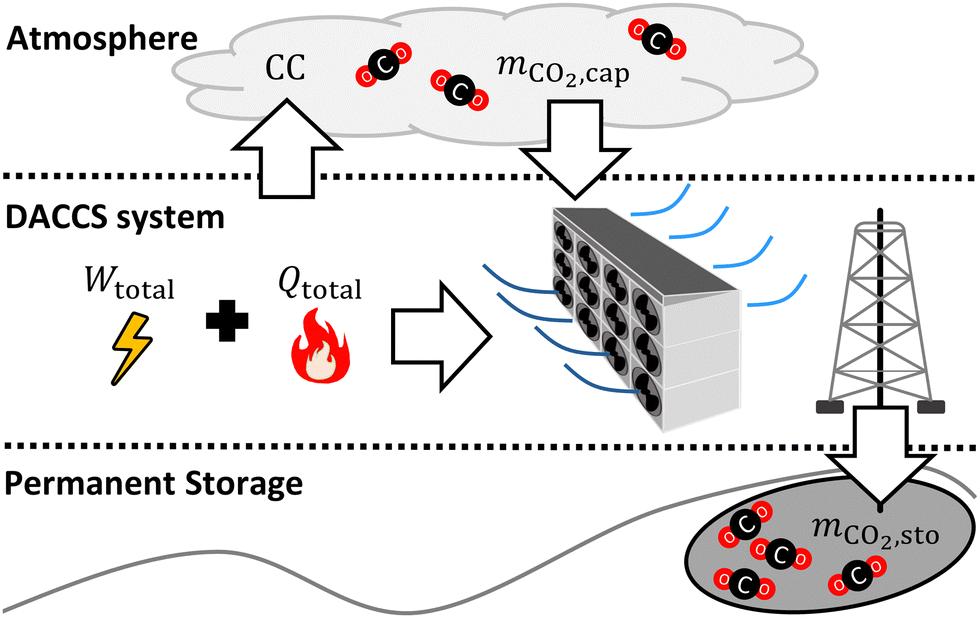 | ||
| Fig. 1 Simplified visualisation of the captured CO2 mass (mco2,cap) and the GHGs emitted (CC) between the atmosphere, the DACCS system, and the permanent storage (mco2,sto). | ||
The specific energy demand (SED), for instance, combines the demand for total work (Wtotal) and total heat (Qtotal) per captured mass of CO2 (mco2,cap):42,46
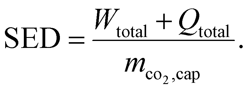 | (1) |
Even if the SED is an intuitive KPI, heat and work are equally weighted, which biases conclusions. From a thermodynamic point of view, the specific exergy demand (SEDex) is more reasonable since it combines the demand for total work and total exergy of heat per captured mass of CO2:
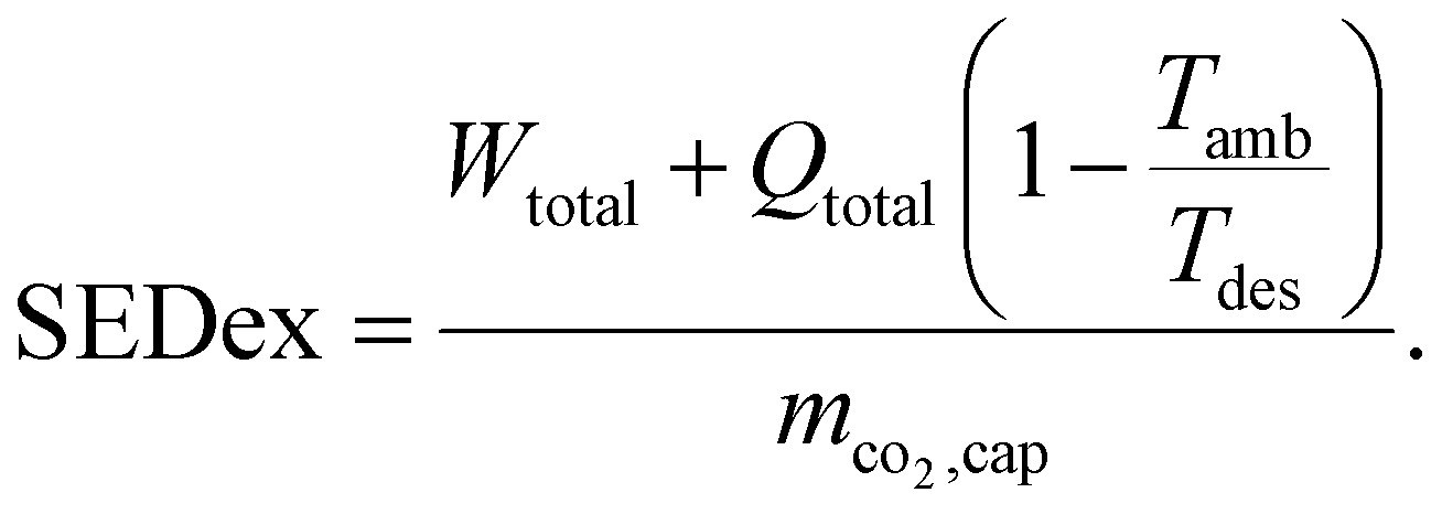 | (2) |
In contrast to the SED, heat is weighted with the exergy fraction 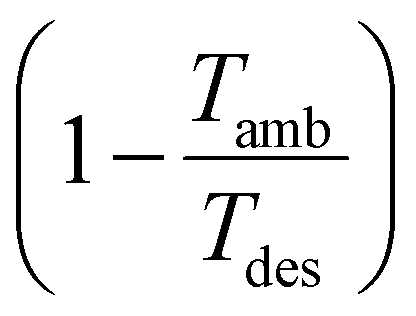 . The exergy fraction is calculated by the Carnot efficiency using the desorption temperature (Tdes) and ambient temperature (Tamb). Using the exergy fraction of heat is a good option from a thermodynamic point of view. However, the ideal conversion from heat to power is unrealistic from a technical point of view. To account for potential conversion losses, the equivalent shaft work (ESW)45,47 is considered, which additionally includes an efficiency for the conversion from heat to power, the exergy efficiency ηex:
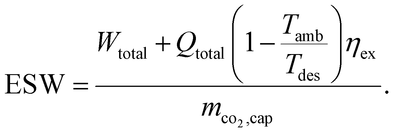 | (3) |
Thus, from a purely technical point of view, the ESW is a good KPI option for processes that require heat and power, such as DACCS.
However, the above-described KPIs neglect the life-cycle GHG emissions and the associated reduction in the net negative emissions of DACCS. To account for that, we use the existing systemic climate-benefit metric carbon removal efficiency (CRE).18 The CRE relates the net negative emissions to the mass of captured CO2. The mass of net negative emissions is the difference between the mass of captured CO2 (mco2,cap) and the climate change (CC) impacts from life-cycle GHG emissions. The total and the specific climate change impacts per mass of captured CO2 (CC and cc, respectively) occur mainly due to the energy supply (CCene), the construction and end-of-life of the DACCS system (CCcons), the adsorbent consumption (CCsor) and possible leakages during transport or storage (CCleak = mco2,cap−mco2,sto). Thus, relevant climate change impacts can be easily taken into account depending on the analysis to be conducted. Overall, the CRE reads as follows:
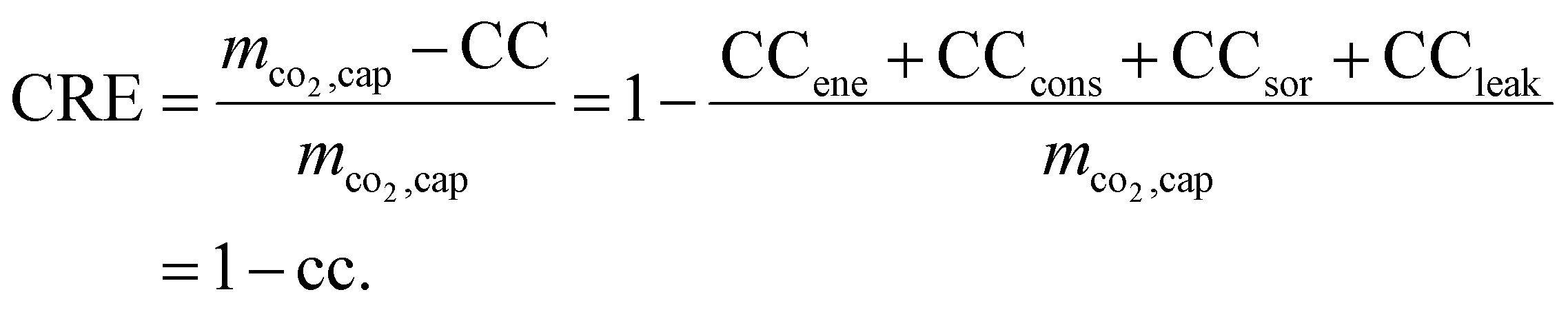 | (4) |
While CCene is a function of the energy demands (Wtotal and Qtotal; cf.eqn (15)), it is obvious that CRE is not just another weighting of Wtotal and Qtotal, since it also takes into account the additional life-cycle emissions from the DACCS system (CCcons and CCsor). The CRE and all other KPIs mentioned can be interpreted as “efficiency”. From thermodynamics, we know a system's efficiency and power usually have a trade-off. The same applies to DACCS: the plant productivity (PP) indicates the “power” of DACCS as it describes the captured CO2 mass per time unit Δτ:41
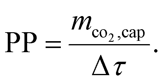 | (5) |
The trade-off between the PP and the “efficiency” KPIs has various reasons. For example, a higher mass flow rate during adsorption results in faster cycles and, thus, in higher PP. However, a higher mass flow rate during adsorption also causes a higher pressure drop and, consequently, a higher energy demand for the fan.
This trade-off between PP and the “efficiency” KPIs cannot be resolved for the energy-related KPIs SED, SEDex and ESW, as the PP cannot be combined with them to a relevant measure. However, the situation is different for the systemic climate-benefit metric CRE. The multiplication of CRE and PP yields a scalar measure showing a DACCS system's carbon removal rate (CRR):
| CRR = PP·CRE. | (6) |
The carbon removal rate indicates the net amount of CO2 that is effectively removed per DACCS system per year.
We discuss all equations for calculating the variables used in the KPIs (Wtotal, Qtotal, CCene, CCcons, CCsor and mco2,cap) in detail in the ESI† and Section 3.1.
3. Modelling and optimisation of a direct air carbon capture and storage system
3.1 Dynamic model of direct air carbon capture and storage system
We based our assessment of the KPIs on a detailed dynamic model of a DACCS system combined with data concerning all life-cycle GHG emissions. The dynamic model (Fig. 2) consisted of four main parts: (i) DAC plant, (ii) recooling, (iii) storage and (iv) energy supply. The parameterised model of the DACCS system will be provided within our open-source Modelica library SorpLib,49 which is publicly available on Gitlab.50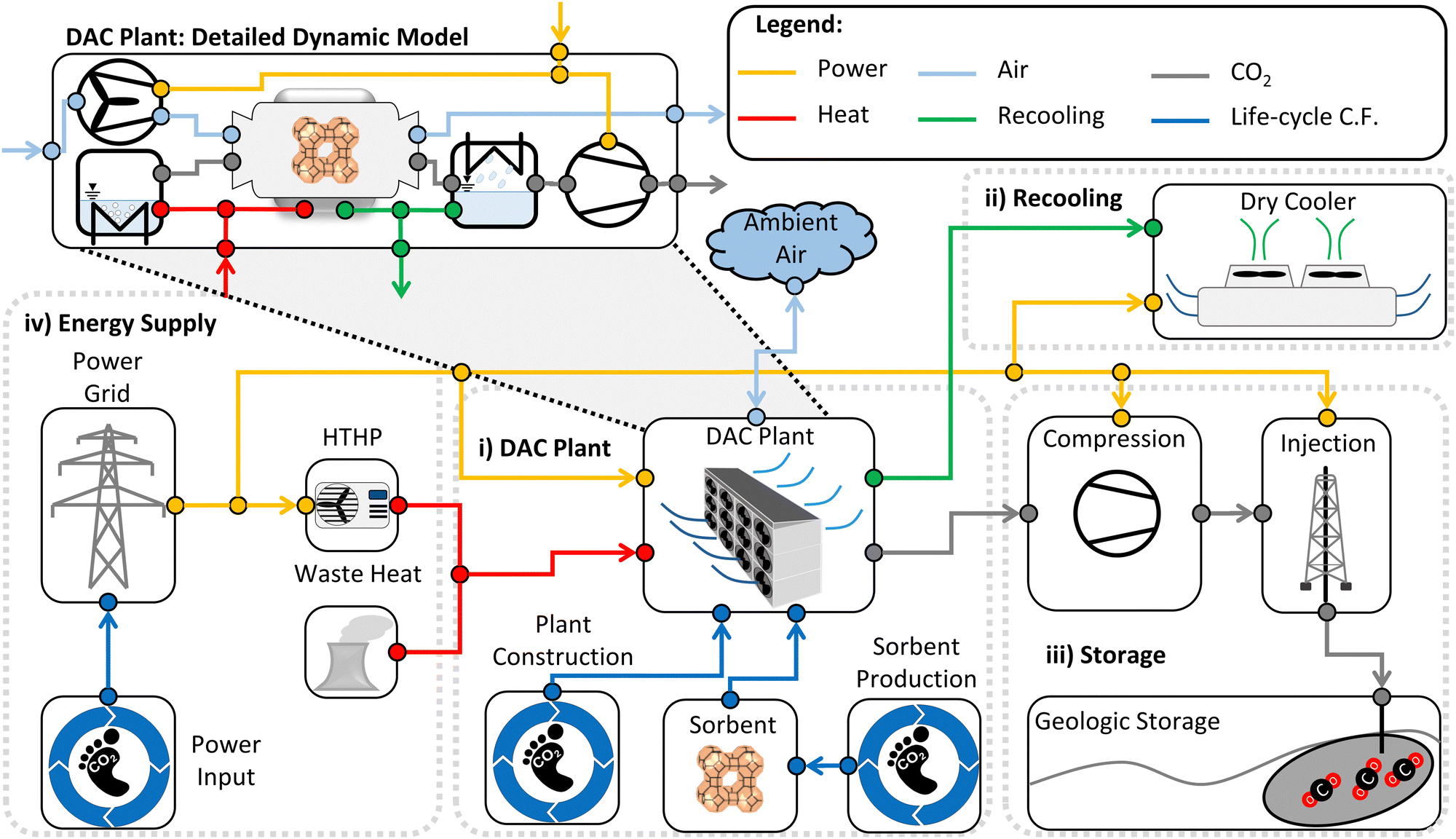 | ||
| Fig. 2 Model scheme of the DACCS system, including its main components and system boundaries. All power flows are marked in yellow, heat flows in red, and waste heat flows in green. The CO2 mass flow rates are marked in grey and ambient air flow rates in light blue. The life-cycle GHG emissions (abbreviated as cc) is shown with blue lines. | ||
The dynamic model of the DAC column is based on a dynamic model of an adsorption column, parameterised (see Section 3.3) for DAC use. We developed a dynamic adsorption column model based on the object-oriented language Modelica51 and the software environment Dymola. We used our open-source Modelica library SorpLib,49 and calculated all fluid properties with the commercial Modelica library TILMedia52 based on RefProp.53 The adsorption column model consisted of four sub-models: (i) gas volume, (ii) adsorbent volume, (iii) wall volume, and (iv) the heat and mass transfers between the sub-models (i)–(iii). We provide a list of the main assumptions and the complete set of equations for all model components in the ESI.†
The DAC column model describes a single column, while a DAC plant combines many columns. Thus, we linearly scaled the performance of the DAC column to a DAC plant with a reference plant productivity PPref of 4 kt CO2 per y. This plant productivity was taken from a reference process (Section 3.4.2). Scaling to a reference plant productivity of 4 kt CO2 per y brings comparability with plants already described and analysed in terms of their environmental impact using a life cycle assessment in the literature.18,19 Deutz and Bardow calculated life-cycle GHG emissions caused by constructing a DAC plant (cccons,DAC) with an annual productivity of 4 kt CO2: they reported 15 kg CO2-eq. per ton captured without equipment recycling and 6 kg CO2-eq. per ton captured with recycling.18 Similar data (6 kg CO2-eq. per ton) was reported by Terlouw et al.19 Thus, we used 6 kg CO2-eq. per ton for our reference process (cccons,DAC,ref). However, the plant productivity changes as the process change. As an approximation, we scaled the life-cycle GHG emissions caused by the construction of the DAC plant linear with plant productivity to calculate the process-dependent emissions:
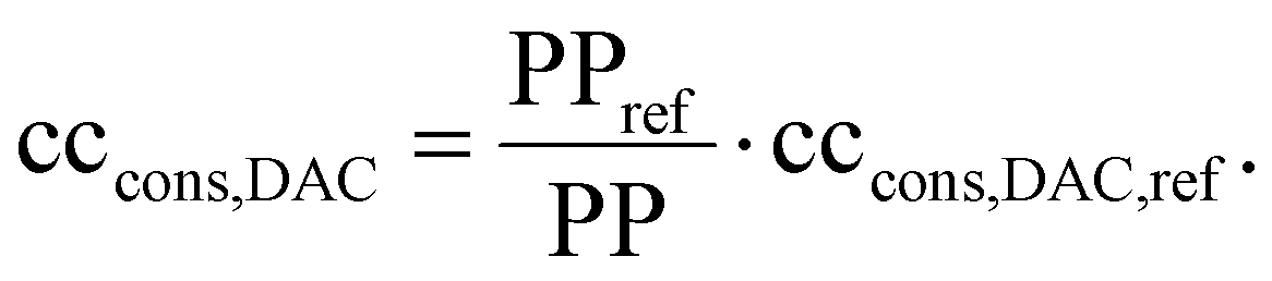 | (7) |
In addition to life-cycle GHG emissions caused by the construction of the DAC plant, emissions are also caused by adsorbent production and consumption. The adsorbent is needed for plant construction and to compensate for degradation. For today's commercial DAC plant operated by Climeworks, 7.5 kg adsorbent per captured ton of CO2 is reported with a prediction of 3 kg adsorbent per captured ton of CO2 for future plants.18 We used a conservative estimate of 7.5 kg adsorbent per captured ton of CO2. For various amine-functionalised adsorbents and an adsorbent consumption of 7.5 kg per captured ton of CO2, life-cycle GHG emissions (ccsor) between 10–46 kg CO2-eq. per ton were reported by Deutz and Bardow,18 which aligns with other studies.19,54 In particular, for amine-functionalised cellulose, the life-cycle GHG emissions are 46 kg CO2-eq. per ton.18 As we used equilibrium and kinetic data of amine-functionalised cellulose (APDES-NFC55) for the dynamic model of the DAC column, we also used the life-cycle GHG emissions reported for amine-functionalised cellulose of 46 kg CO2-eq. per ton.
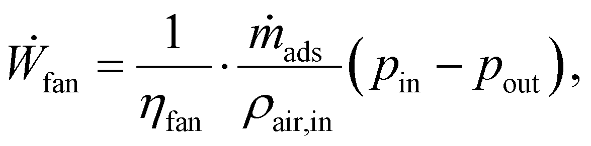
The DAC plant also has auxiliary components to run the cyclic batch process (cf. Section 3.2): a fan moves ambient air through the adsorption column in the adsorption phase. Fan's power consumption (Ẇfan) was modelled as an isothermal, steady-flow process with an incompressible fluid. An incompressible fluid was assumed because the pressure change from the fan is so small that the density remains constant. Hence, the fan's power consumption41
 | (8) |
Another auxiliary component is the steam generator for steam-assisted desorption. The required heat flow rate (![[Q with combining dot above]](https://www.rsc.org/images/entities/i_char_0051_0307.gif) ste) for steam generation,
ste) for steam generation,
| ste = ṁste(hs,H2O(Tdes,pdes) − hl,H2O(Tamb,pdes)), | (9) |
In addition to the steam generator, a recooler/condenser cools the hot and humid mass flow leaving the adsorption column (ṁdes) to ambient temperature and condensing excess water (ṁcon). The product mass flow rate (ṁpro) is the difference between desorbed and condensed mass flow rate (ṁpro = ṁdes − ṁcon). The heat flow rate in the recooler/condenser (cond) was expressed as:
| con = ṁdeshmix,des(Tdes,pdes) − ṁprohmix,pro(Tamb,pdes) − ṁconhl,H2O(Tamb,pdes), | (10) |
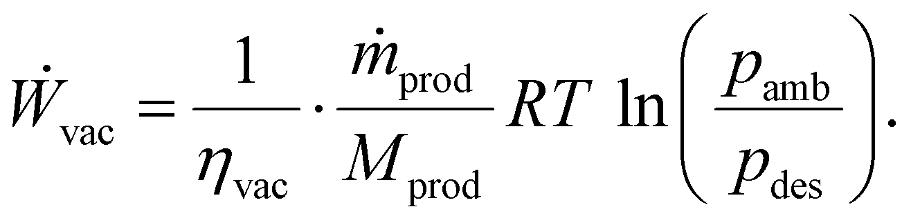
The last auxiliary component of the DAC plant is a vacuum pump, which lowers the pressure in the adsorption column for desorption. We modelled the power consumption of the vacuum pump (Ẇvac) as an isothermal compression of an ideal gas in a steady-state flow process:41
 | (11) |
For calculating the power consumption of the vacuum pump, we used the vacuum pump efficiency (ηvac), the molar mass of the product mixture (Mprod), and the ambient pressure (pamb).
| Wrecool = 0.045 Qrecool. | (12) |
This simple correlation is valid for the heat rejection of chillers (30–40 °C). Nevertheless, we assumed the temperature gradient is inherently more significant for the heat rejection of the DACCS system, making it a conservative estimate of the work required.
Regardless of the transport route length, the CO2 has to be compressed. We modelled the energy demand of this compression as an isothermal, steady flow compression of an ideal gas:58
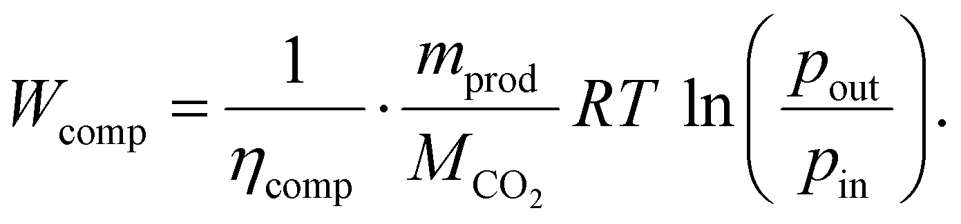 | (13) |
As suggested in the literature, we replaced the factor containing the ideal gas constant (R), the temperature (T), the molar mass (MCO2), and the compressor efficiency (ηcomp) with a constant value of 87.85 kJ kg−1.58 The compressed mass of the product (mprod) includes the total mass of captured CO2 (mco2,cap) and all remaining impurities. Thus, the specific energy demand is 114 kW h-el. per t for the compression of a ton of product from ambient pressure to a pipeline pressure of 110 bar.
In line with Terlouw et al., we assumed a depth of 2000 m for the geological storage site, which results in an injection pressure of 216 bar.19 Therefore, 16 kW h-el. per t is required for the compression from the pipeline to the storage pressure (eqn (13)).
The heat supply was divided into two scenarios. In the first scenario, a high-temperature heat pump (HTHP) used electricity from the power grid to supply heat. The power consumption of the HTHP was proportional to the total heat flow rate (total) and was calculated with the maximal theoretical heat pump efficiency and an exergy efficiency (ηex,HTHP) as:18
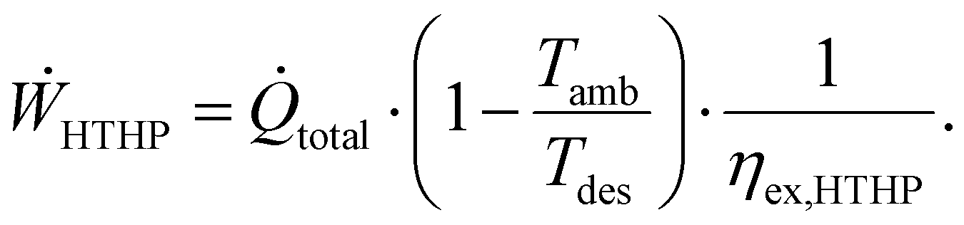 | (14) |
The GHG emissions of the production and end-of-life of the HTHP are very small compared to the overall life-cycle emissions of a DACCS system,19 and we neglected GHG emissions from the HTHP other than electricity induced. The second scenario uses waste heat (WH) for heat supply. We assumed unlimited availability of the waste heat up to 100 °C and to be burden-free, i.e., waste heat does not cause any GHG emissions. In both scenarios for heat supply, energy-related GHG emissions are caused only by electricity supply. Thus, overall GHG emission from energy supply can be calculated from the total electricity demand (Wtotal) and the electricity's GHG emissions (cfel) as:
| ccene = cfelWtotal. | (15) |
We vary the electricity's GHG emissions (cfel) in a given range to fully cover all possible scenarios or geographical specifications for electricity supply.
Equations for calculating the total electricity demand (Wtotal) and the total heat demand (Qtotal) for the DACCS system are discussed in the ESI.†
3.2 Investigated adsorption cycle for direct air capture
The process of DAC can be described in terms of the adsorption cycle. Adsorption cycles for gas separation are mainly characterised by their regeneration method:59• Temperature swing: a higher temperature leads to lower equilibrium loading and, thus, to desorption.
• Pressure (or vacuum) swing: a lower (partial) pressure leads to lower equilibrium loading and, thus, to desorption. The cycle is called a vacuum swing if the total pressure is below ambient.
• Concentration swing: the mechanism is identical to the pressure swing (i.e., low partial pressure) but achieved by injecting an inert gas or steam.
• Desorption displacement: the adsorbate is displaced by another adsorptive with a higher or similar affinity.
The regeneration methods are often combined: e.g., a temperature vacuum swing adsorption cycle (TVSA) combines the temperature and vacuum swing as regeneration methods. The TVSA is one of the most popular cycles for DAC15 and is already used in commercial DACCS systems.28 The TVSA is recommended for high CO2 purities of 95–99.9%.60 In addition to the TVSA, the steam-assisted temperature vacuum swing adsorption cycle (S-TVSA) is studied in the literature for high CO2 purities as well.41,44,46 In the S-TVSA, a concentration swing via a steam purge is combined with a temperature and vacuum swing. According to the literature, the S-TVSA can outperform the TVSA regarding productivity.41,44 As the steam in the S-TVSA can be easily removed by condensation, TVSA and S-TVSA are the two most promising cycles for DACCS when requiring high CO2 purities for efficient transportation and storage. Therefore, we investigated both the TVSA and S-TVSA. Following Young et al.,45 we used the TVSA and the S-TVSA described by Stampi-Bombelli et al.,41 but extended by a cooling phase to reduce adsorbent degradation. Hence, both cycles had five phases: (i) adsorption, (ii) blowdown, (iii) heating, (iv) desorption, and (v) cooling (Fig. 3). Both cycles are identical except for the desorption phase where the S-TVSA is purged with a mass flow rate of superheated steam, but the TVSA is not. The ESI† provides a detailed explanation of both cycles and their five phases.
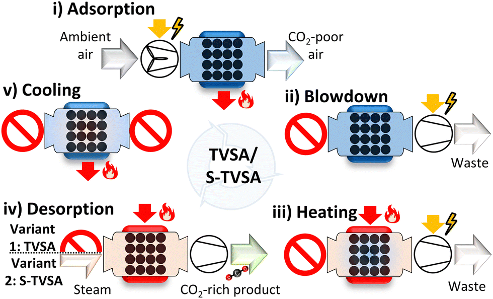 | ||
| Fig. 3 The five phases of a temperature vacuum swing adsorption cycle (TVSA) and a steam-assisted temperature vacuum swing adsorption cycle (S-TVSA) applied for DAC are adapted from Young et al. and Stampi-Bombelli et al.31,35 (i) Adsorption: a fan blows ambient air through the adsorption column; CO2 and H2O are adsorbed. (ii) Blowdown: a vacuum pump decreases the column pressure to desorption pressure as the column inlet is closed. (iii) Heating: a jacket heats the column to the desorption temperature. (iv) Desorption via the TVSA cycle: extraction of CO2 with closed column inlet; desorption via the S-TVSA: extraction of CO2 by injecting superheated steam. (v) Cooling: ccooling of the adsorption column to below 90 °C. | ||
3.3 Parameterisation and validation of the dynamic adsorption column model
For parameterising the dynamic adsorption column model for DAC applications, the following data is crucial: (i) co-adsorption equilibrium model and data, (ii) kinetic data (heat and mass transfer), (iii) column geometries, and (iv) pressure drop correlations. We used the complete set of required data for a dynamic model published by Stampi-Bombelli et al.41 We examined amine-functionalised cellulose APDES-NFC as the adsorbent, which was assumed to only adsorb H2O and CO2.41 To model the co-adsorption equilibrium of H2O and CO2, we used a modified Toth-isotherm model for the CO2 and a Guggenheim–Anderson de Boer isotherm for the H2O. The equations and their parameters are taken from the literature41 and are given in the ESI.† The kinetics are defined by (i) the mass transport between the gas volume and the adsorbent cell and (ii) heat transfers between all components. We used published kinetic parameters from the literature41 based on experimental breakthrough curves61 and desorption experiments.62 The geometric data and model parameters characterising the adsorption column were also taken from the literature.41 The pressure drop of a fluid flow through a porous medium in packed bed columns is typically modelled with the Ergun equation63 or similar equations.64 A particular form of the Ergun equation is the Kozeny–Carman equation, characterised by minor deviations from the Ergun equation for low velocities but higher numerical efficiency. Numerical efficiency is essential for optimisation, especially when optimising complex systems like the used DACCS model. Therefore, we calculated the pressure drop with the Kozeny–Carman equation instead of the Ergun equation.All details of data used for parameterisation and a comparison with the literature model by Stampi-Bombelli et al.41 are given in the ESI.†
3.4 Case study, reference process, and optimisation framework
With Sections 3.1–3.3, the DACCS system model is fully defined and can be evaluated using the KPIs from Section 2. However, the adsorption cycle (i.e., TVSA and S-TVSA, cf. Section 3.2) and the heat source (i.e., WH or HTHP, cf. Section 3.1), strongly affect the KPIs. To be able to examine the effects separately, we defined different scenarios investigated in this work.Besides the differences between the four possible cases, some parameters were identical for all cases and defined our case study. The same parameters for all cases are, e.g., environmental conditions such as temperature or relative humidity, the plant construction's life-cycle GHG emissions, and the DACCS system's configuration. A complete list of all parameters defining the case study is available in the ESI.† Furthermore, we assumed that the DAC plant and the storage site are nearby. Then, no off-site pipelines would need to be built and operated. In addition, we assumed no leakage during transportation or storage. However, impacts from pipelines and leakages can be easily integrated into our method in future detailed analyses if corresponding data are available (see eqn (4)).
The DAC plant model represented the Climeworks process very well with only minor deviations: The specific heat demand was approximately 3.8 kW h-th. kg per CO2, the specific power demand was approx. 0.7 kW h-el. kg per CO2 and the cycle time was 6.5 h. However, our model had a slightly higher specific heat demand. The higher specific heat demand can be caused by several factors such as differences in the ambient conditions, in the equilibrium loadings of the adsorbent, in inert thermal mass (i.e., column design), or the enthalpy of adsorption. Particularly, differences in the ambient conditions must be mentioned: slight differences in the ambient air's relative humidity already significantly influence the specific heat requirement and, thus, the overall process performance.66,67 In addition to the specific heat demand, the cycle time is slightly longer, with 6.5 h compared to 6 h which could be explained e.g., by different kinetics.
For the identified reference process, the resulting column productivity was used as a reference and was set equal to plant productivity of 4 kt CO2 per y. Thus, we linearly scaled up from column productivity to plant productivity. For the reference process of the S-TVSA, we used the same process as for the TVSA. In addition, the S-TVSA has a steam mass flow rate during the desorption phase. We used the same steam mass flow rate as Stampi-Bombelli et al. in their base case.41 The complete set of process variables of the S-TVSA is given in the ESI.†
 | (16) |
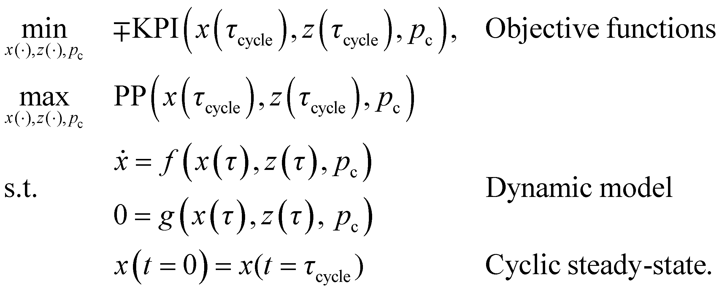
The KPIs SED, SEDex, and ESW were minimised, and CRE was maximised. Simultaneously, plant productivity (PP) was maximised. As constraints, the optimisation problem had the differential-algebraic system of equations of the dynamic DACCS model and a cyclic steady-state condition. All differential states of the dynamic model are annotated by x, the algebraic states in z, and the process variables in pc. The process variables are the degrees of freedom for the optimisation and are the mass flow rate (ṁads) during adsorption, the phase times (τads, τheat, and τdes), as well as desorption conditions (pdes, Tdes, and ṁstea). A table with all process variables, as well as their lower and upper bounds, for the optimisation, is included in the ESI.†
As described in Section 2, there is also the option of resolving the trade-off for CRE and PP by forming the product, i.e. CRR. Then, the bi-objective optimisation problem from eqn (16) is simplified to the following single-objective optimisation problem:
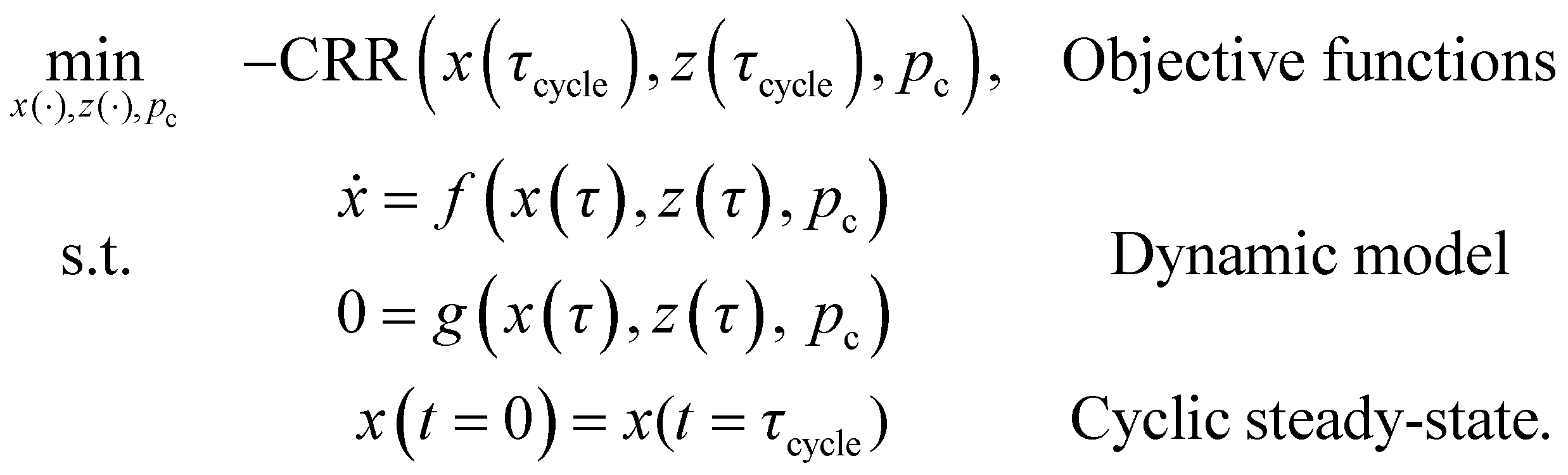 | (17) |
To solve the bi-objective and the single-objective optimisation problem, we exported the dynamic DACCS model as a functional mock-up unit using the functional mock-up interface.68 The exported model was coupled with the genetic optimisation algorithms within the Python package Pymoo.69 To solve the bi-objective optimisation problem we used the NSGAII70 algorithm and to solve the single-objective optimisation problem we used a particle swarm optimisation.71
4. Results
We first present an analysis of the reference process to validate our model and identify first insights for process analysis (Section 4.1). Next, we show the results of the process optimisation using different KPIs (Section 4.2). Finally, we show the influence of the GHG emissions from electricity supply (Section 4.3).4.1 Analysis of the reference process
Fig. 4 shows the SED of the reference process (Section 3.4.2) for the TVSA applied in (a) a DAC plant and (b) a DACCS system. The DACCS system requires only 3% more energy than the DAC plant. Similar results were obtained for the S-TVSA reference process (cf. ESI†). The DAC plant and DACCS system require mainly heat and comparatively low power. Regarding power consumption, the fan is the largest consumer for the TVSA, followed by the vacuum pump and the power consumption for recooling. In the total energy demand for the DACCS system, the power demands for the compression and the injection of CO2 into the storage sites (2.44% and 0.35%, respectively) have only minor importance (Fig. 4(b)). However, even if storage is not particularly relevant from an energy perspective, this changes when life-cycle GHG emissions are considered.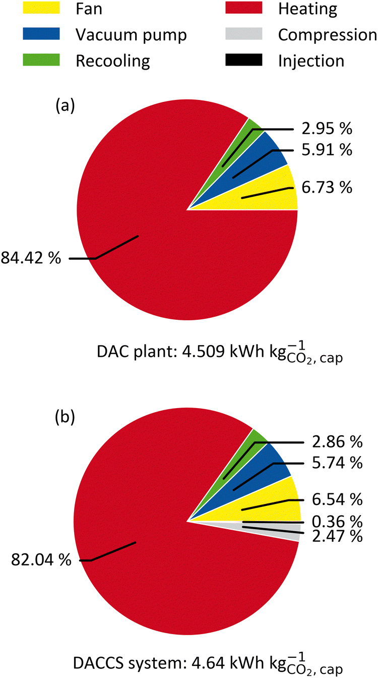 | ||
| Fig. 4 Specific energy demands of (a) a DAC plant and of (b) a DACCS system based on a TVSA for the reference process. The plant productivity is 4 kt CO2 per y. The specific energy demands are divided into the demands heat (red), power for the fan (yellow), power for the vacuum pump (blue), and power for recooling (green). For the DACCS system, the power demands for the compression and the injection into the storage site are added in grey and black, respectively. | ||
To investigate impairments of a purely energetic analysis, we calculated the GHG emissions per captured mass of CO2 (cc) caused by the removal process. Remember, the specific GHG emissions (cc) can easily be converted into the CRE and vice versa (cf.eqn (4)).
The system boundaries for the DACCS system are defined in Fig. 2. In a base case, we used the electricity GHG emissions of Switzerland (0.166 kg CO2-eq. per kW h-el.) since one of the first commercial DAC systems was established in Switzerland.18Fig. 5 shows the specific GHG emissions for a DACCS system based on a TVSA and operated by (a) WH or (b) a HTHP for the reference process. The specific GHG emissions are 0.19 kg CO2-eq. per kg for the WH case, which corresponds to a CRE of 81%. This CRE aligns with life cycle assessment studies of similar waste-heat-powered DACCS systems with the same electricity GHG emissions.18,19 The specific life-cycle GHG emissions for the HTHP case are 0.44 kg CO2-eq. per kg, which corresponds to a CRE of 56%. This CRE also agrees with other studies of similar DACCS systems.18,19
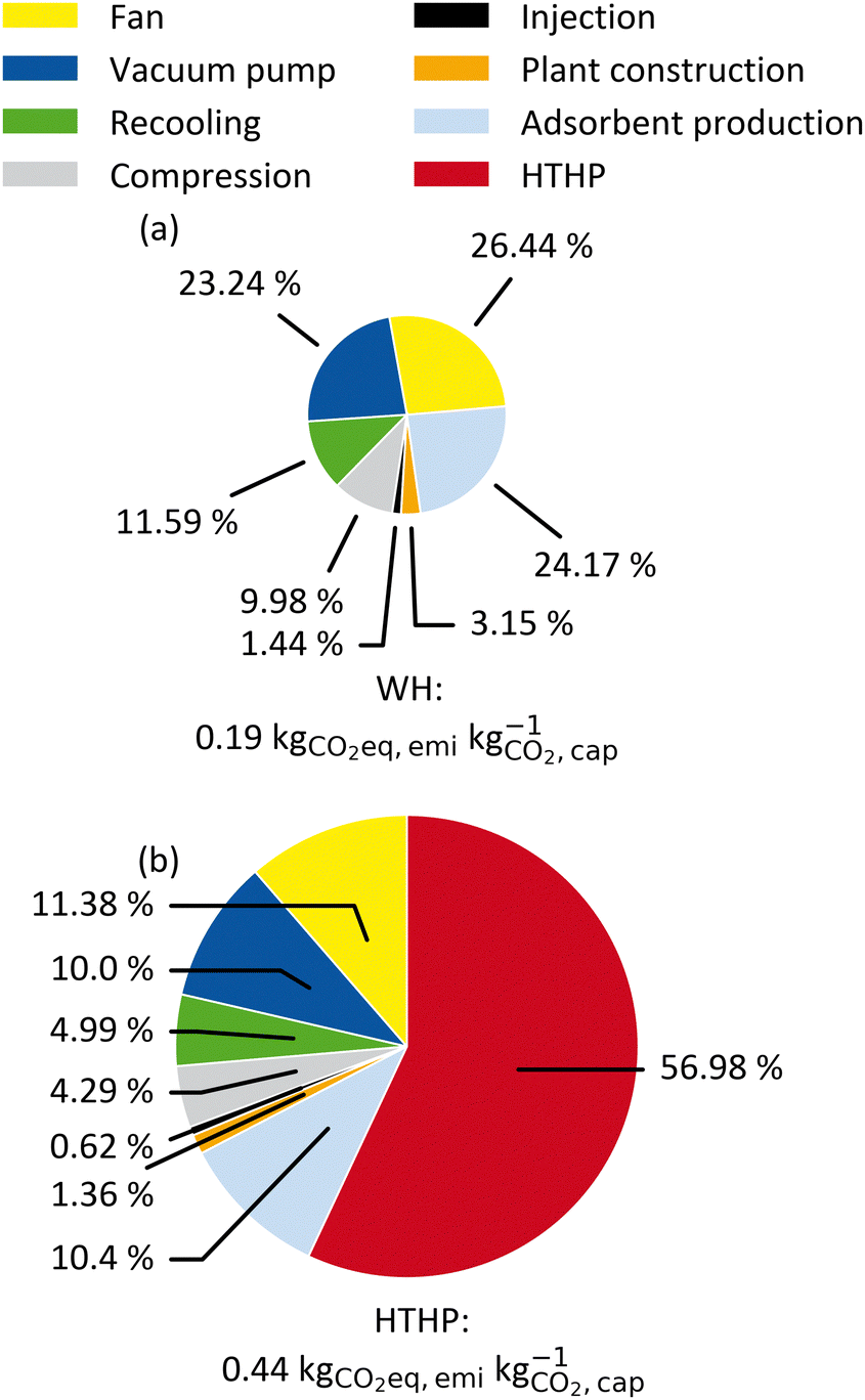 | ||
| Fig. 5 GHG emissions during the removal process for a DACCS system based on a TVSA cycle. Values are given for the reference process with plant productivity of 4 kt CO2 per y: (a) WH case and (b) HTHP case. The electricity's GHG emissions are 0.166 kg CO2-eq. per kW h-el. | ||
In addition to the TVSA, we calculated the specific GHG emission for a DACCS system based on a S-TVSA (ESI†). The WH: S-TVSA has specific GHG emissions of 0.23 kg CO2-eq. per kg, which corresponds to a CRE of 77%. For HTHP: S-TVSA, specific GHG emissions are 0.49 kg CO2-eq. per kg, corresponding to a CRE of 51%. The specific GHG emission of the DACCS system based on the S-TVSA increase by 21% for the WH case and 11% for the HTHP case compared to the TVSA cycle. At the same time, the plant productivity PP increases from 4.0 to 4.12 kt CO2 per y for the S-TVSA cycle compared to the TVSA cycle.
An analysis of the DACCS system, as shown in Fig. 4 and 5, can be used to evaluate the system and identify bottlenecks. However, a sound KPI must be used to avoid incorrect conclusions. For instance, storage does not seem relevant when considered in terms of the SED (Fig. 4(b)) but accounts for up to 11% of specific GHG emissions (Fig. 5(a)). Accordingly, the KPIs selection is crucial for evaluating a fixed process. The following section examines the impact of KPI selection on DACCS process optimisation.
4.2 The impact of the KPI used for process optimisation
To highlight the impact of the KPI selection in process optimisation, Fig. 6 shows results using different KPIs, with CRE and plant productivity (PP) on the axes. The processes were optimised for the four “efficiency” KPIs (CRE, ESW, SEDex, and SED) and PP (cf.eqn (16)). Each process optimisation results in a different Pareto frontier. For a Pareto frontier using, e.g., CRE as “efficiency” KPI, we refer to as CRE-optimal in the following. The corresponding process variables for each Pareto frontier can be found in the ESI.† Although each optimisation yields a distinct Pareto frontier, not all are depicted as such. Fig. 6 shows all Pareto frontiers using CRE and PP on the axes. Hence, only the CRE-optimal processes are aligned with the “correct” axes. For instance, the SED-optimal processes should be plotted with SED and PP on the axes. Despite the unconventional approach of showing Pareto frontiers with varying axes, Fig. 6 compares all Pareto frontiers regarding their CRE.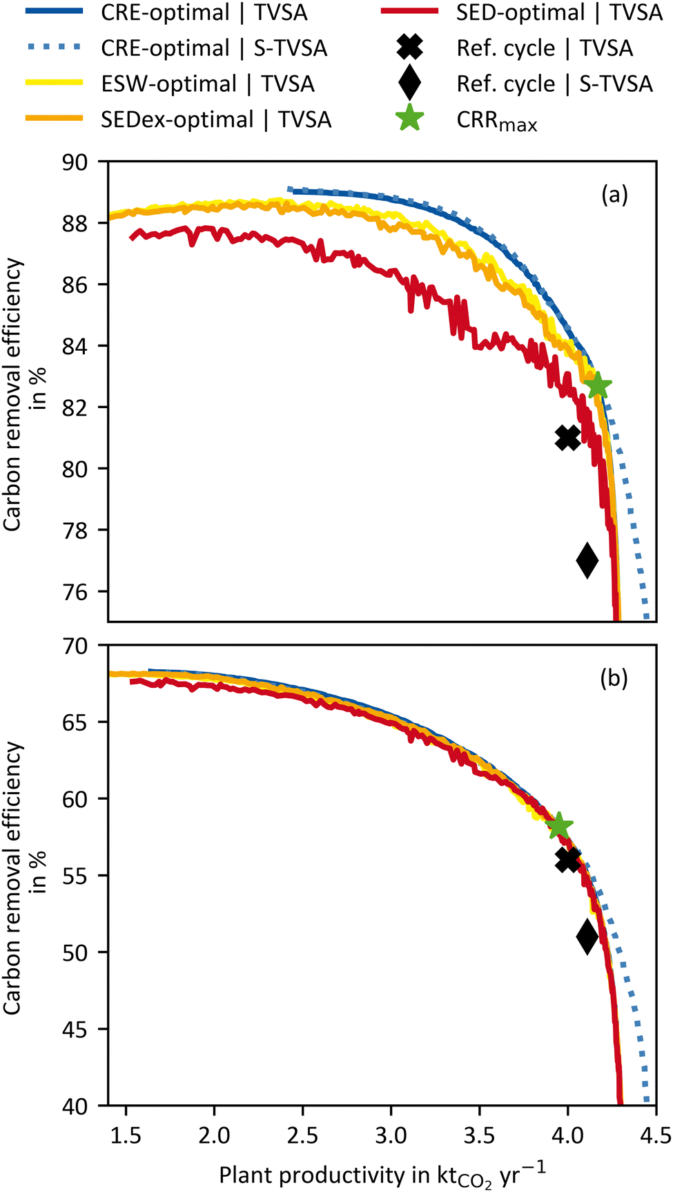 | ||
| Fig. 6 Trade-offs between plant productivity and carbon removal efficiency for different KPI-optimal processes: (a) WH case and (b) HTHP case. Solid lines relate to the TVSA cycle and dashed lines to the S-TVSA cycle. The electricity's GHG emissions are 0.166 kg CO2-eq. per kW h-el. | ||
For the WH case (Fig. 6(a)), it is evident that the SED-optimal (i.e., Pareto frontiers using SED) processes have the lowest CRE over the entire plant productivity range. For example, at the plant productivity of 3.5 kt CO2 per y, the CRE-optimal process has a CRE of 87.8%, and the SED-optimal has a CRE of 83.9%, which corresponds to a reduction in CRE of more than 4%. On average, the SEDex- and ESW-optimal processes outperform the SED-optimal processes, and their CREs deviate by approx. 1% from the CRE-optimal processes over a large plant productivity range. The ESW-optimal processes always slightly outperform the SEDex-optimal processes because the conversion losses between heat and electricity were included in the calculation (see eqn (3)). Thus, heat in the ESW is weighted even less than in the SEDex, which brings it closer to the actual waste heat case. In summary, the CRE of the DACCS system could be increased using the CRE as a KPI for process optimisation instead of the energy-related KPIs (ESW, SEDex, and SED).
The most significant advantage of the CRE as a KPI becomes apparent when looking at the upper left end of each Pareto frontier, where the “efficiency” KPIs are maximal. For an energy-intensive process such as DACCS, the use of the “most efficient” process seems reasonable from the outset, but clearly shows the limitations of the state-of-the-art KPIs (ESW, SEDex, and SED). For the CRE-optimal processes, the maximal achievable carbon removal efficiency (CREmax) is 89% reached at a plant productivity of approximately 2.5 kt CO2 per y. Thus, lower plant productivities than 2.5 kt CO2 per y are not on the CRE Pareto frontier, leading to a simultaneous decline in plant productivity and the CRE. Consequently, a process leading to plant productivity below 2.5 kt CO2 per y is never advisable from an environmental point of view. Nonetheless, the ESW-, SEDex-, and SED-optimal processes have their maxima (ESWmax, SEDexmax, and SEDmax, respectively) at way lower plant productivities of 1.42, 1.42, and 1.54 kt CO2 per y, respectively. These lower plant productivities result from the plant construction included in the CRE. As the share of the overall GHG emissions from plant production is lower for higher plant productivity, the trade-off between CRE and PP is reduced. The reduction of the trade-off becomes even more relevant when lower carbon energy sources are used because the CREmax shifts further towards higher plant productivity. However, as this trade-off reduction only appears for the CRE, the maxima of the ESW-, SEDex- and SED-optimal processes are shifted towards smaller plant productivity. The inherent characteristics of Pareto frontiers cause both CRE and plant productivity to decrease for all non-CRE-optimal process. For example, in Fig. 6(a), the process leading to ESWmax (at CRE = 88.3% and PP = 1.42 kt CO2 per y) is 0.8% worse in terms of CRE and, at the same time, 42.3% worse in terms of plant productivity compared to the process leading to CREmax (at CRE = 89.0% and PP = 2.46 kt CO2 per y). The comparison of the “most efficient” processes (CREmax with ESWmax, SEDexmax, and SEDmax) admittedly leads to the worst performance of the state-of-the-art KPIs compared to CRE. While this comparison might seem unfair when having the full Pareto frontiers available, such comparison might be drawn when optimising DACCS processes for a single objective of “energy efficiency” (ESWmax, SEDexmax, and SEDmax). We will use the comparison of “most efficient” processes as one extreme case to highlight the potential for unexploited climate benefits when using the wrong KPIs.
Fig. 6(b) shows the same Pareto frontiers as (a), but for the HTHP case. As for the WH case, all non-CRE-optimal process are worse in CRE and plant productivity than in the CRE-optimal process. It is important to note that the ESW-, SEDex-, and SED-optimal processes are exactly the same for the HTHP case (Fig. 6(b)) as for the WH case (Fig. 6(a)) because the state-of-the-art KPIs do not distinguish where the heat comes from. However, the same processes lead to different CRE values due to the change in the heat source. The deviations between the different Pareto frontiers are smaller for the HTHP case than for the WH case. This can be attributed to heat being responsible for the most GHG emissions in the HTHP case (cf.Fig. 5(b)). The KPIs CRE, ESW, SEDex, and SED all include a heat share, which is weighted differently in each KPI. For the HTHP case, the weighting between heat and electricity is very similar for the CRE and ESW. Therefore, the ESW-optimal process is the next best after the CRE-optimal process. The SED-optimal process shows the most significant deviation from the CRE-optimal process. The equal weighting of heat and electricity in the SED significantly differs from the weighting in the CRE of the HTHP case. However, with deviations below 1%, this is only marginal over the complete plant productivity range.
Looking at the shift to smaller plant productivity for the HTHP case, it is apparent that it is much lower than for the WH case. For the HTHP case, the smaller shifts in plant productivity are attributed to the lower contribution of plant construction to overall GHG emissions. Nevertheless, the plant productivity of the process leading to the ESWmax (at CRE = 68.1% and PP = 1.42 kt CO2 per y) is about 13.4% smaller than the process leading to the CREmax (at CRE = 68.3% and PP =1.64 kt CO2 per y).
In addition to the effects of the KPIs on the Pareto frontiers, Fig. 6(a) and (b) also show a comparison between a DACCS system based on a TVSA and S-TVSA. For a better overview, for the S-TVSA, only the CRE-optimal process is shown, as qualitative results do not differ for the other KPIs. The TVSA and S-TVSA have the same performance over a wide plant productivity range for both the WH and HTHP cases. The same performance is caused by the steam mass flow rate, which is set to its lower bound by the optimisation for a large plant productivity range. Thus, the S-TVSA cycle becomes de facto a TVSA, and the S-TVSA offers no advantages regarding CRE for low plant productivity. Even though the S-TVSA did not require such low desorption pressures, the additional energy required for recooling outweighs the higher desorption pressure. However, it is notable that the S-TVSA outperforms the TVSA regarding the maximal plant productivity for both cases, which aligns with other literature.41,44 The S-TVSA increases the maximal achievable plant productivity from 4.31 kt CO2 per y to 4.5 kt CO2 per y (not shown in Fig. 6) with the same CRE due to the following reasons: (i) the driving force for mass transport increases during desorption caused by reducing the partial pressure of the CO2 in the adsorption column and (ii) faster heating caused by the direct contact of the adsorbent with the superheated steam.
From Fig. 6, we can conclude the following: CRE for process optimisation is a reasonable KPI and leads to a shift of the Pareto frontier both in the direction of a higher CRE and in the direction of higher plant productivity. We show that this is true for the WH case and the HTHP case, but the effects are weaker for the WH case. Further, it can be noted that the shift to higher plant productivity is significant, which means that using state-of-the-art KPIs for process optimisation leaves enormous carbon removal potential unused. For the shift to higher plant productivity, we show that the intensity of the shift depends on the share of emissions from DACCS system construction (CCcons) in total emissions (CC). This raises the question of whether emissions from energy supply (CCene) and mostly from electricity's GHG emissions also influence the shift of the CRE-optimal Pareto frontier to higher CRE and plant productivity. We will examine the impact of GHG emissions from electricity supply in the following section.
4.3 The impact of electricity's GHG emissions
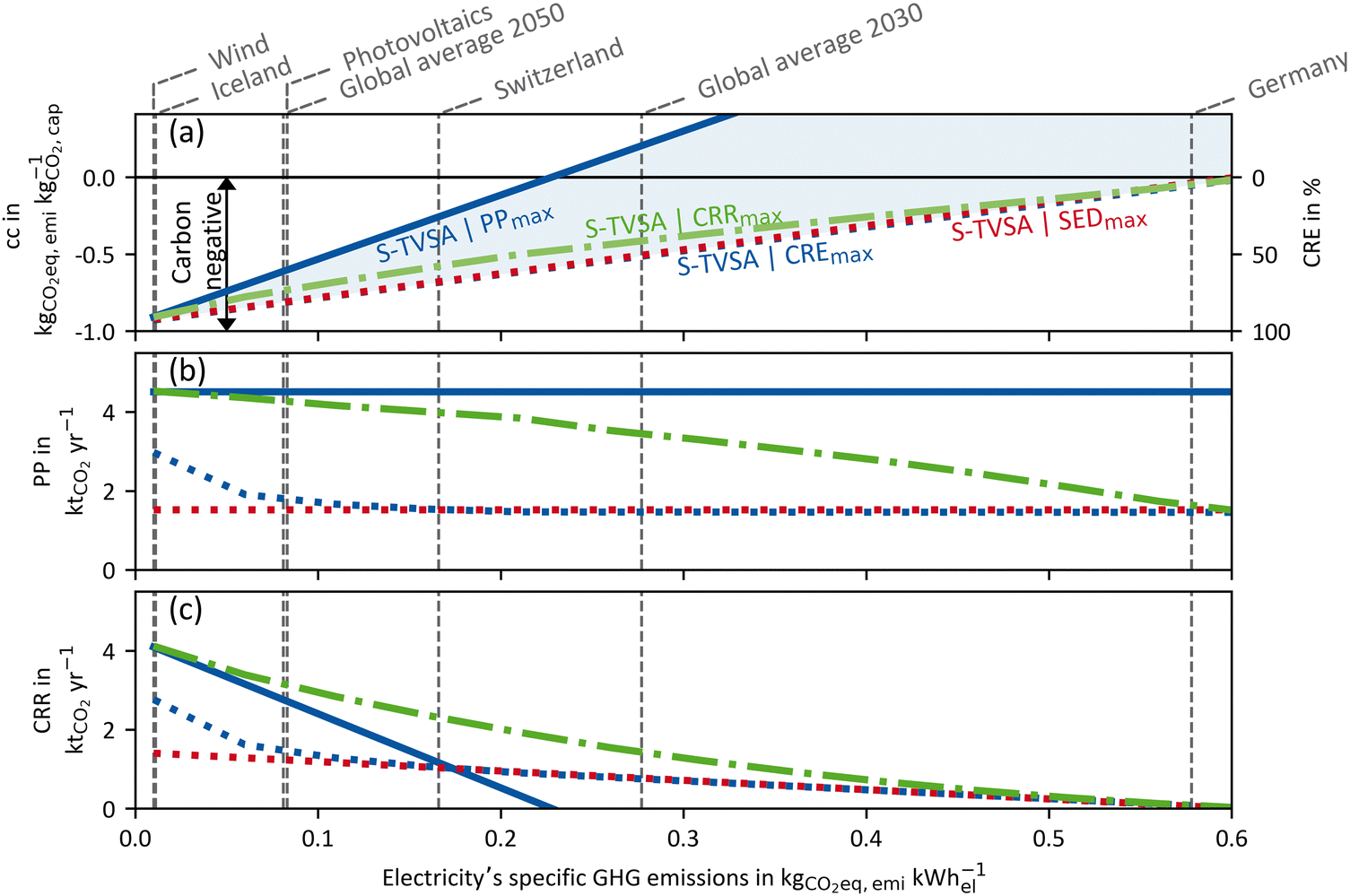
To examine the impact of the electricity's GHG emissions (cfel, cf.eqn (15)), we vary cfel and calculate new Pareto frontiers comparable to Fig. 6 for each given value ranging from 0.01–0.6 kg CO2-eq. per kW h-el. However, we do not use the entire Pareto frontier but reduce each Pareto frontier to two points. The first point is the maximal achievable “efficiency” KPI process (e.g. CREmax) at the upper left end of each Pareto frontier (cf.Fig. 6). The other point is the maximum plant productivity process (PPmax) at the lower right edge of each Pareto frontier (cf.Fig. 6). Each point contains a CRE and a PP value. Thus, for each electricity's GHG emission, these two points of the Pareto frontier cover the possible operation range of a Pareto-optimal DACCS system. From these data, we derive Fig. 7 (waste heat case) and Fig. 8 (heat pump case) by plotting CRE and PP over the electricity's GHG emissions in each sub-plot (a). The boundary of the operation range for the maximal achievable plant productivity (PPmax) is visualised as a solid line, and the boundary for the maximal achievable “efficiency” KPI as a dashed line. Different colours of the lines refer to different “efficiency” KPIs used for the optimisation, where blue indicates CRE and red indicates SED. The maximum carbon removal rate (CRRmax) eqn (17) is also included as a green dash-dot line. Fig. 7 and 8(a) have two ordinates: the GHG emissions per captured mass of CO2 (cc) are plotted on the primary ordinate, and the CRE on the secondary ordinate. To better interpret the electricity's GHG emissions, we have included vertical lines, which show cfel in different scenarios or locations.18 Further, we show only the S-TVSA, as it only extends the operating range of the TVSA cycle to higher plant productivity (cf.Fig. 6). Thus, the operating range of the TVSA cycle is included in the operating range of the S-TVSA cycle.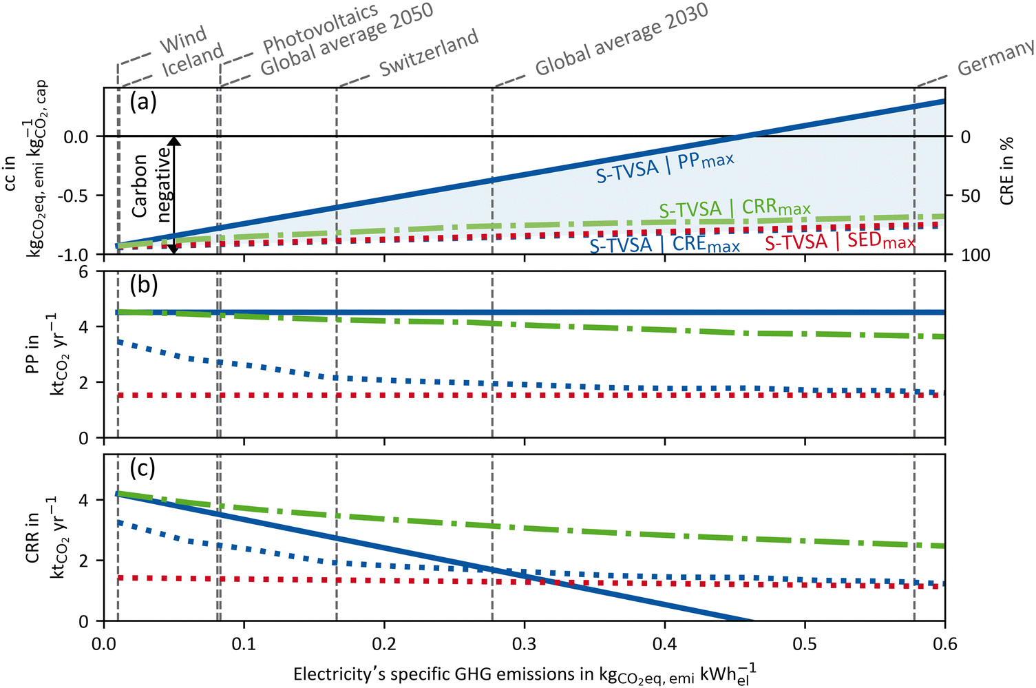 | ||
| Fig. 7 WH case: (a) GHG emissions per captured mass of CO2 (primary ordinate, left), carbon removal efficiency (secondary ordinate, right), (b) plant productivity and (c) the carbon removal rate dependent of the electricity's GHG emissions for a DACCS system based on the S-TVSA cycle. The solid blue line marks the process leading to PPmax, and the dashed lines the processes leading to CREmax (blue) and SEDmax (red), respectively. Further, green dash-dot lines show the process leading to CRRmax. Grey vertical dashed lines mark defined electricity's GHG emissions for different scenarios or locations.33 | ||
 | ||
| Fig. 8 HTHP case: (a) GHG emissions per captured mass of CO2 (primary ordinate, left), carbon removal efficiency (secondary ordinate, right), (b) plant productivity and (c) the carbon removal rate dependent of the electricity's GHG emissions for a DACCS system based on the S-TVSA cycle. The solid blue line marks the process leading to PPmax, and the dashed lines the processes leading to CREmax (blue) and SEDmax (red), respectively. Further, green dash-dot lines show the process leading to CRRmax. Grey vertical dashed lines mark defined electricity's GHG emissions for different scenarios or locations.33 | ||
WastehHeat case: as seen in Fig. 7 for the waste heat scenario, the CRE for all processes is almost linearly dependent on the electricity's GHG emissions. Further, the process leading to the SEDmax has only slightly lower CRE than the CREmax. Regarding the CRE at electricity's GHG emissions close to zero, it becomes apparent that the CRE did not reach 100%. The construction emissions of the DACCS system and the adsorbent consumption cause this emission offset even if electricity was burden–free. For a process leading to PPmax, a positive CRE was possible over a large range of electricity's GHG emissions. A positive CRE indicates that more CO2 is captured than emitted; thus, the aim of DACCS to generate net negative emissions is met. The break-even point for net negative emissions is 0.457 kg CO2-eq. per kW h-el. for the WH case and the process leading to PPmax. If the electricity is more GHG intense, the process leading to PPmax could not fulfil the aim of net CO2 removal. Then, more CO2 is emitted than captured. In contrast, the CRE for the processes leading to the SEDmax, CREmax and CRRmax are positive over the entire range of the electricity's GHG emissions. However, the price to pay for that is lower plant productivity, discussed in detail in the next paragraph.
In addition to the GHG emissions per captured mass of CO2 (cc), we show the plant productivity in Fig. 7(b). The plant productivity for the process leading to PPmax remains constant, which is reasonable since the GHG emissions of the electricity do not affect the maximal plant productivity. Further, it is noticeable that the plant productivity remains constant for the process with SEDmax as well. In contrast, the plant productivity for the process leading to CREmax depends strongly on the GHG emissions of the electricity. For low electricity GHG emissions, the plant productivity for the process leading to CREmax is almost equal to the process leading to PPmax. This is reasonable, as for burden-free electricity (cfel = 0), the plant construction and the adsorbent consumption are the only GHG emissions from the entire DACCS system. Even though adsorbent production is independent of the process, the percentage of plant construction of total emissions decreases with increasing plant productivity. Therefore, the trade-off between CRE and PP is mitigated with lower GHG emissions for electricity supply. Theoretically, for burden-free electricity, the plant productivity process leading to CREmax tends to equal the maximal plant productivity. However, we have only calculated results for electricity's GHG emissions as little as 0.01 kg CO2-eq. per kW h-el. For high GHG emissions of electricity, the plant productivity of the process leading to CREmax approaches the plant productivity of the process leading to SEDmax. Hence, the lower the electricity's GHG emissions, the larger the difference in the plant productivity for a process leading to CREmax compared to SEDmax. Looking at the process leading to CRRmax, this process is noticeable that it has very high plant productivities for the complete range of the electricity's GHG emissions. For clean electricity, the plant productivities of the processes leading to PPmax and CRRmax are almost identical, and the plant productivity of the CRRmax process declines only slightly and nearly linearly with rising electricity's GHG emissions (cf.Fig. 7(b)). The disadvantage of the process leading to CRRmax is a slightly lower CRE compared to the processes leading to CREmax and SEDmax (cf.Fig. 7(a)).
We observed that CRE is quite similar for processes leading to SEDmax, CREmax and CRRmax (deviations always below 12%). However, plant productivity differs substantially for these processes: the CRRmax process can always achieve high plant productivities, close to the theoretical maximum of PPmax = 4.5 kt CO2 per y; the SEDmax process achieves only PP = 1.54 kt CO2 per y (deviations between CRRmax and SEDmax design in PP are always larger than 58%). Therefore, we can deduce that for high CRR, a high PP might be more important than a high CRE. Obviously, highest CRR is obtained by the optimisation with CRR as KPI (CRRmax). The difference between the CRRmax process and other processes in Fig. 7(c) can be interpreted as the unexploited carbon removal potential. It is important to note that the unexploited carbon removal potential in Fig. 7(c) represents a worst-case scenario, as the analysis is confined to the limits of the Pareto frontiers. Although the unused potential may be less significant along the rest of the Pareto frontiers, this worst-case scenario highlights the potential unexploited carbon removal potential even with processes that are on the Pareto frontier.
High-temperature heat pump case: similar to Fig. 7 and 8 shows the results for the HTHP case. The process leading to PPmax already emits more CO2 than it captures at electricity GHG emissions of about 0.2 kg CO2-eq. per kW h-el. Even for the processes leading to the CREmax and SEDmax, the CRE becomes negative at 0.6 kg CO2-eq. per kW h-el. Thus, regardless of the process, more CO2 is emitted than captured with the modelled DACCS system for cfel > 0.6 kg CO2-eq. per kW h-el. Overall, the process is even more crucial for the HTHP case than for the WH case, as large parts of the operation range are in the negative CRE range. For the HTHP case, the trends for the plant productivity over the electricity's GHG emissions (of Fig. 8(b)) are equal but less intense than those for the WH case. For low GHG emissions of electricity, the plant productivity of the process leading to CREmax tends to maximal plant productivity. In contrast, for high GHG emissions of electricity, the plant productivity of the process leading to CREmax is equal to the plant productivity of the process leading to SEDmax. A direct comparison of plant productivities of the WH case and the HTHP case (Fig. 7(b) and 8(b)) shows a steeper slope of the plant productivity for the HTHP case. The slope is steeper because the GHG emissions share of plant construction in the HTHP case decreases more rapidly with increasing GHG emissions of electricity as, in total, more electricity is required.
Fig. 7 and 8 show one of the major strengths of combining a detailed dynamic process model with using CRE as KPI for DACCS. The purpose of DACCS is net negative emissions, and from the CRE, it can be directly concluded whether this purpose is met or not. However, net negative emissions do not mean using DACCS is the best option for using “clean” energy. For example, the potential for emissions reduction could be higher if “clean” electricity is used in heat pumps to replace oil-fired domestic heating. However, such a competitive technology analysis for the best possible use of “clean energy”72 in terms of climate benefit is out of scope of this work, but the developed method enables such an assessment in future analyses. Regardless of whether there is a possible more sustainable use case for the energy used for DACCS, the CRE directly shows whether net negative emissions are possible with the electricity, heat source, and process used. Net negative emissions can be achieved for the WH and the HTHP case with the modelled DACCS system. However, for both cases, there are specific break-even points for the electricity's GHG emissions, for which negative emissions become impossible (CRE < 0). Even if negative emissions are already achieved at moderate GHG electricity emissions of less than 0.2 kg CO2-eq. per kW h-el. for all cases and all Pareto-optimal processes, the practical use of DACCS may become effective with even “cleaner” electricity, with “effective” meaning that meaningful amounts of CO2 are actually removed. For example, even a CRE of 50% means that for every ton of CO2 that is actually removed from the atmosphere, two tons must be captured and stored to compensate for the life-cycle emissions. Moreover, the KPI choice for process optimisation is particularly crucial, especially for low GHG electricity emissions. As shown in Fig. 7 and 8, the plant productivity of the CREmax process increases strongly for low cfel while the plant productivity for the SEDmax process remains constant. Thus, the state-of-the-art KPIs (e.g. SED) lead to large unused carbon removal potential, especially when the electricity becomes “cleaner”, which is necessary for reasonable employment of DACCS.
The state-of-the-art KPIs, SED, SEDex, and ESW are always in a trade-off with plant productivity PP. Therefore, we have also looked at the same trade-off between CRE and PP in Section 4.2. Nevertheless, the CRE offers the decisive advantage that the product of CRE and PP, i.e., the CRR, represents the net amount of CO2 removed per time unit. The CRR reduces the Pareto frontier to a scalar objective function for process optimisation without significant information losses. Especially for extensive sensitivity studies, such a scalar quantity is better suited and more accessible to interpret. Due to the scalar dimension, there is no need to discuss a whole Pareto frontier as there is only one single best process.
As shown in Fig. 7 and 8, the processes leading to CRRmax is a process that leads to high PP for “cleaner” electricity. This high PP is achieved primarily through short cycle durations. However, in addition to decreasing the cycle duration, the CRRmax process also switches from a TVSA to a S-TVSA to further increase PP (Fig. 9). For electricity's GHG emissions above 0.3 kg CO2-eq. per kW h-el., the process leading to CRRmax is a TVSA cycle for both the WH and the HTHP case, and the mass flow rate of steam is at the lower boundary. With decreasing electricity's GHG emissions, the process switches from a TVSA to a S-TVSA for both cases. The steam mass flow rate is heading towards the upper limit, because a higher steam mass flow rate increases the plant productivity PP. Fig. 9 shows that the optimal process is a function of the electricity's GHG emissions, a new relevant insight for operating a DACCS system. The new insight suggests that in an energy system where the GHG emissions of the electricity change, varying the process is likely to increase the performance of DACCS. This finding would not be possible with the state-of-the-art KPIs and highlights the importance of combining a detailed dynamic DACCS model and LCA data to leverage the full carbon removal potential of DACCS.
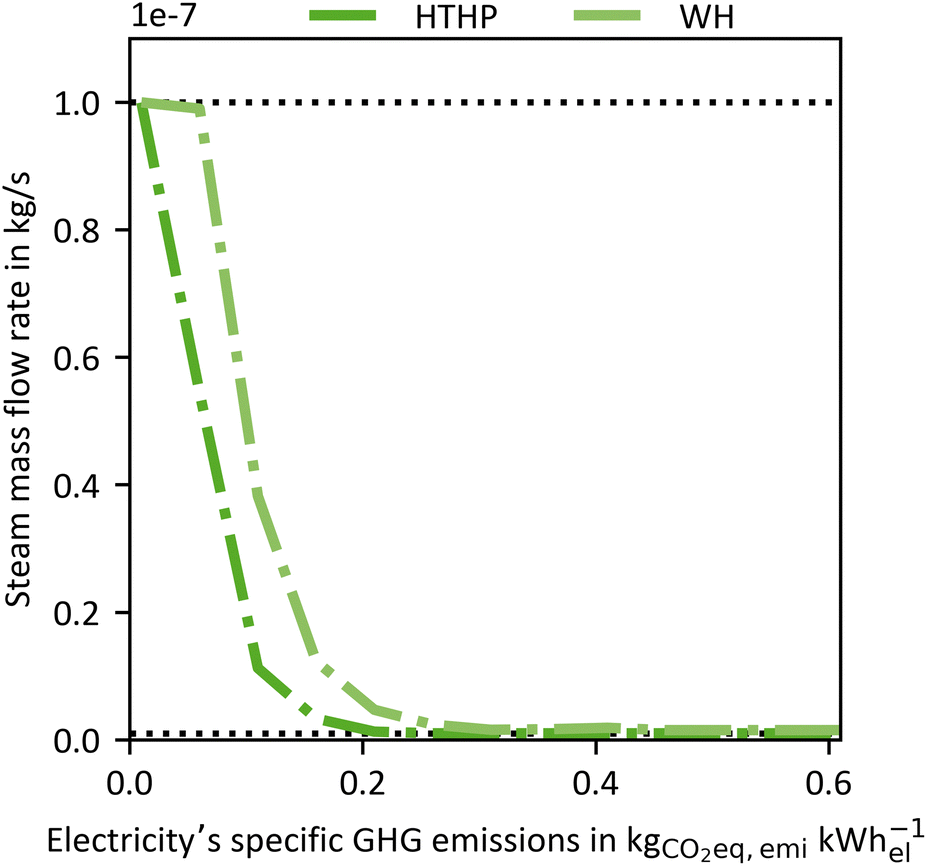 | ||
| Fig. 9 Steam mass flow rate of the process leading to the maximal carbon removal rate CRRmax plotted over the electricity's greenhouse gas (GHG) emissions for a DACCS system for the waste heat (WH) and the high-temperature heat pump (HTHP) case. | ||
5. Conclusion
This work aims to improve the state-of-the-art for evaluating and optimising DACCS. Common approaches are either a purely technical analysis based on detailed process models, or an environmental analysis based on static black-box models. Detailed process models allow for deep insights into the process and process optimisations but fail to quantify the aim of DACCS: net removing CO2 from the atmosphere. Instead, these detailed process models use technical performance metrics such as specific energy demand, specific exergy demand, equivalent shaft work and plant productivity (PP). In contrast, static black-box models do not allow for detailed process analyses and process optimisations. However, they can assess DACCS regarding the net removed CO2 by considering all life-cycle GHG emissions. These life cycle assessment-based analyses of DACCS allow for calculating the systemic climate-benefit metric carbon removal efficiency (CRE). The CRE gives the share of net CO2 removed per CO2 captured, i.e., how much of the captured CO2 is effectively removed from the atmosphere after subtracting all life-cycle GHG emissions.To overcome the limitations of both approaches, we extended a detailed dynamic DACCS process model to cover all life-cycle GHG emissions. Extending the DACCS process model to include life-cycle GHG emissions increases the model's complexity and also demands more data. In return, this extension enables the use of systemic climate-benefit metrics like the CRE for detailed process analysis and process optimisation. Thus, our approach enables a comprehensive assessment of DACCS and makes the CRE accessible for detailed process analyses and process optimisations for the first time.
The extended DACCS model enables a process optimisation with respect to various “efficiency” KPIs as well as PP. As “efficiency” KPIs, we used (i) specific energy demand, (ii) specific exergy demand, (iii) equivalent shaft work, and (iv) CRE. To reflect the trade-off between the four KPIs and PP, we solved the process optimisation as four individual bi-objective optimisation problems, yielding Pareto frontiers. For a temperature vacuum swing adsorption cycle, the Pareto frontier from using CRE as KPI is shifted toward higher CRE and higher PP compared to the Pareto frontiers using the other KPIs. Thus, the CRE-optimal processes always outperform the processes using other KPIs. The shift towards higher CRE for the same plant productivity depends on the cases for heat and electricity supply, but this shift to higher CRE is generally small (below 4%). The shift towards higher plant productivity, however, is much more significant and relevant for the overall carbon removal potential.
As example, for forecasted global average electricity GHG emissions for 2030 and a heat supply from waste heat, the lowest plant productivity still on the Pareto frontier is 1.94 kt CO2 per y when using CRE as objective function (cf.Fig. 7). With the same power and heat supply but using the specific energy demand as KPI for process optimisation, the lowest plant productivity still on the Pareto frontier is 1.52 kt CO2 per y. The higher plant productivity for CRE-based optimisation results to an unexploited potential of 0.42 kt CO2 per y (+28%) for the same DACCS system. We show that the effect of underestimating the plant productivity becomes even more significant with decreasing GHG emissions of electricity. For the forecasted global average electricity GHG emissions for 2050, this unexploited potential increases up to 1.2 kt CO2 per y.
We strongly recommend using systemic climate-benefit metrics as KPIs for process optimisation and evaluation of DACCS to fully exploit its carbon removal potential. A benefit of making systemic climate-benefit metrics accessible as KPIs for process optimisation is that it allows the resolution of the trade-off with PP by using the carbon removal rate (CRR), which is the product of CRE and PP. CRR indicates the net amount of CO2 that is effectively removed per DACCS system per year. Thus, only one single best process exists that maximises the CRR, and Pareto frontiers with multiple optimal processes are avoided. Moreover, CRR is particularly suitable for large sensitivity studies, as we did regarding the impact of electricity GHG emissions on the optimal process design. We showed that the CRR maximal process design changes from a temperature vacuum swing to a steam-assisted temperature vacuum swing adsorption cycle when electricity gets “cleaner”. Bearing in mind that the optimal process is a function of the electricity's GHG emissions, a DACCS system should be operated flexibly in an energy system with varying GHG emissions of the electricity. Further research is required to clarify the effects of flexible DACCS operation in volatile energy systems. Furthermore, a cost assessment should be combined with the presented optimisation approach to identify DACCS systems that can be scaled to maximal CO2 removal potential at lowest costs. We suggest combining CRE and carbon removal costs for economic assessment.
Which of the two systemic climate-benefit metrics (CRE or CRR) is advisable depends on the analyses; for example, CRR is particularly suitable for large sensitivity studies, as the trade-off with the PP is resolved, and CRE is suited for combination with further KPIs, e.g. in economic analyses. In any case, the KPIs must reflect the goal of DACCS: effectively removing CO2 from the atmosphere. This general principle applies to adsorption-based DACCS, as we have investigated in this work, and to all negative emission technologies. Hence, we recommend applying our combined approach of model-based process optimisation using systemic climate-benefit metrics as KPI to other DACCS processes and negative emission technologies in general.
Author contributions
Patrik Postweiler contributed to the conceptualisation, data curation, software, formal analysis, investigation, visualisation, methodology, and writing – original draft. Mirko Engelpracht contributed to the conceptualisation, data curation, software, methodology, and writing – review & editing. Daniel Rezo contributed to the data curation, validation, and writing – review & editing. Andrej Gibelhaus contributed to the conceptualisation and writing – review & editing. Niklas von der Assen contributed to the conceptualisation, resources, supervision, funding acquisition, project administration, and writing – review & editing.Conflicts of interest
There are no conflicts to declare.Acknowledgements
We gratefully acknowledge the financial support from the German Federal Ministry for Education and Research (BMBF) in the founding initiative “KMU-innovativ” via the project MoGaTEx (01LY2001B). Simulations were performed with computing resources granted by RWTH Aachen University under project rwth0769.References
- UNFCCC, ed., Paris Agreement to the United Nations Framework Convention on Climate Change, 2015, COP 21.
- IPCC, ed., Climate Change 2022: Mitigation of Climate Change. Contribution of Working Group III to the Sixth Assessment Report of the Intergovernmental Panel on Climate Change, Cambridge University Press, Cambridge, UK and New York, NY, USA, 2022.
- S. Fawzy, A. I. Osman, J. Doran and D. W. Rooney, Environ. Chem. Lett., 2020, 18, 2069–2094 CrossRef CAS.
- G. Realmonte, L. Drouet, A. Gambhir, J. Glynn, A. Hawkes, A. C. Köberle and M. Tavoni, Nat. Commun., 2019, 10, 3277 CrossRef CAS PubMed.
- G. F. Nemet, M. W. Callaghan, F. Creutzig, S. Fuss, J. Hartmann, J. Hilaire, W. F. Lamb, J. C. Minx, S. Rogers and P. Smith, Environ. Res. Lett., 2018, 13, 63003 CrossRef.
- J. DeAngelo, I. Azevedo, J. Bistline, L. Clarke, G. Luderer, E. Byers and S. J. Davis, Nat. Commun., 2021, 12, 6096 CrossRef CAS PubMed.
- J. Rogelj, A. Popp, K. V. Calvin, G. Luderer, J. Emmerling, D. Gernaat, S. Fujimori, J. Strefler, T. Hasegawa, G. Marangoni, V. Krey, E. Kriegler, K. Riahi, D. P. van Vuuren, J. Doelman, L. Drouet, J. Edmonds, O. Fricko, M. Harmsen, P. Havlík, F. Humpenöder, E. Stehfest and M. Tavoni, Nat. Clim. Change, 2018, 8, 325–332 CrossRef CAS.
- C. Chen and M. Tavoni, Clim. Change, 2013, 118, 59–72 CrossRef CAS.
- Committee on Developing a Research Agenda for Carbon Dioxide Removal and Reliable Sequestration, Board on Atmospheric Sciences and Climate, Board on Energy and Environmental Systems, Board on Agriculture and Natural Resources, Board on Earth Sciences and Resources, Board on Chemical Sciences and Technology, Ocean Studies Board, Division on Earth and Life Studies, National Academies of Sciences, Engineering and Medicine, Negative Emissions Technologies and Reliable Sequestration: A Research Agenda, Washington (DC), 2018.
- J. C. Minx, W. F. Lamb, M. W. Callaghan, S. Fuss, J. Hilaire, F. Creutzig, T. Amann, T. Beringer, W. de Oliveira Garcia, J. Hartmann, T. Khanna, D. Lenzi, G. Luderer, G. F. Nemet, J. Rogelj, P. Smith, J. L. Vicente Vicente, J. Wilcox and M. del Mar Zamora Dominguez, Environ. Res. Lett., 2018, 13, 63001 CrossRef.
- S. Fuss, W. F. Lamb, M. W. Callaghan, J. Hilaire, F. Creutzig, T. Amann, T. Beringer, W. de Oliveira Garcia, J. Hartmann, T. Khanna, G. Luderer, G. F. Nemet, J. Rogelj, P. Smith, J. L. V. Vicente, J. Wilcox, M. del Mar Zamora Dominguez and J. C. Minx, Environ. Res. Lett., 2018, 13, 63002 CrossRef.
- M. Z. Jacobson, Energy Environ. Sci., 2019, 12, 3567–3574 RSC.
- T. Terlouw, C. Bauer, L. Rosa and M. Mazzotti, Energy Environ. Sci., 2021, 14, 1701–1721 RSC.
- S. Fuss, J. G. Canadell, P. Ciais, R. B. Jackson, C. D. Jones, A. Lyngfelt, G. P. Peters and D. P. van Vuuren, One Earth, 2020, 3, 145–149 CrossRef.
- N. McQueen, K. V. Gomes, C. McCormick, K. Blumanthal, M. Pisciotta and J. Wilcox, Prog. Energy, 2021, 3, 32001 CrossRef.
- J. Fuhrman, H. McJeon, P. Patel, S. C. Doney, W. M. Shobe and A. F. Clarens, Nat. Clim. Change, 2020, 10, 920–927 CrossRef CAS.
- V. Heck, D. Gerten, W. Lucht and A. Popp, Nat. Clim. Change, 2018, 8, 151–155 CrossRef CAS.
- S. Deutz and A. Bardow, Nat. Energy, 2021, 6, 203–213 CrossRef CAS.
- T. Terlouw, K. Treyer, C. Bauer and M. Mazzotti, Environ. Sci. Technol., 2021, 55, 11397–11411 CrossRef CAS PubMed.
- S. Smith, O. Geden, G. F. Nemet, M. Gidden, W. F. Lamb, C. Powis, R. Bellamy, M. Callaghan, A. Cowie, E. Cox, S. Fuss, T. Gasser, G. Grassi, J. Greene, S. Lueck, A. Mohan, F. Müller-Hansen, G. Peters, Y. Pratama, T. Repke, K. Riahi, F. Schenuit, J. Steinhauser, J. Strefler, J. Maria Valenzuela and J. Minx,State of Carbon Dioxide Removal, 1st edn, 2023 Search PubMed.
- M. Fasihi, O. Efimova and C. Breyer, J. Cleaner Prod., 2019, 224, 957–980 CrossRef CAS.
- E. S. Sanz-Pérez, C. R. Murdock, S. A. Didas and C. W. Jones, Chem. Rev., 2016, 116, 11840–11876 CrossRef PubMed.
- M. Yang, C. Ma, M. Xu, S. Wang and L. Xu, Curr. Pollut. Rep., 2019, 5, 272–293 CrossRef CAS.
- M. Erans, E. S. Sanz-Pérez, D. P. Hanak, Z. Clulow, D. M. Reiner and G. A. Mutch, Energy Environ. Sci., 2022, 15, 1360–1405 RSC.
- N. von der Assen, L. J. Müller, A. Steingrube, P. Voll and A. Bardow, Environ. Sci. Technol., 2016, 50, 1093–1101 CrossRef CAS PubMed.
- P. Jaramillo, W. M. Griffin and S. T. McCoy, Environ. Sci. Technol., 2009, 43, 8027–8032 CrossRef CAS PubMed.
- H. Ostovari, L. Müller, J. Skocek and A. Bardow, Environ. Sci. Technol., 2021, 55, 5212–5223 CrossRef CAS PubMed.
- C. Beuttler, L. Charles and J. Wurzbacher, Front. Clim., 2019, 1, 3 CrossRef.
- F. Sabatino, A. Grimm, F. Gallucci, M. van Sint Annaland, G. J. Kramer and M. Gazzani, Joule, 2021, 5, 2047–2076 CrossRef CAS.
- D. W. Keith, G. Holmes, D. St. Angelo and K. Heidel, Joule, 2018, 2, 1573–1594 CrossRef CAS.
- C. Gebald, J. A. Wurzbacher, P. Tingaut, T. Zimmermann and A. Steinfeld, Environ. Sci. Technol., 2011, 45, 9101–9108 CrossRef CAS PubMed.
- T. Gelles, S. Lawson, A. A. Rownaghi and F. Rezaei, Adsorption, 2020, 26, 5–50 CrossRef CAS.
- X. Shi, H. Xiao, H. Azarabadi, J. Song, X. Wu, X. Chen and K. S. Lackner, Angew. Chem., Int. Ed., 2020, 59, 6984–7006 CrossRef CAS PubMed.
- A. Kumar, D. G. Madden, M. Lusi, K.-J. Chen, E. A. Daniels, T. Curtin, J. J. Perry and M. J. Zaworotko, Angew. Chem., Int. Ed., 2015, 54, 14372–14377 CrossRef CAS PubMed.
- M. Schellevis, T. Jacobs and W. Brilman, Front. Chem. Eng., 2020, 2, 6907 Search PubMed.
- Q. Yu and W. Brilman, Appl. Sci., 2020, 10, 1080 CrossRef CAS.
- E. Bachman, A. Tavasoli, T. A. Hatton, C. T. Maravelias, E. Haites, P. Styring, A. Aspuru-Guzik, J. MacIntosh and G. Ozin, Joule, 2022, 6, 1368–1381 CrossRef CAS.
- D. Marinič and B. Likozar, J. Cleaner Prod., 2023, 408, 137185 CrossRef.
- K. Madhu, S. Pauliuk, S. Dhathri and F. Creutzig, Nat. Energy, 2021, 6, 1035–1044 CrossRef CAS.
- P. Goglio, A. G. Williams, N. Balta-Ozkan, N. R. P. Harris, P. Williamson, D. Huisingh, Z. Zhang and M. Tavoni, J. Cleaner Prod., 2020, 244, 118896 CrossRef.
- V. Stampi-Bombelli, M. van der Spek and M. Mazzotti, Adsorption, 2020, 1183–1197 CrossRef CAS.
- M. Schellevis, T. N. van Schagen and D. W. F. Brilman, Int. J. Greenhouse Gas Control, 2021, 110, 103431 CrossRef.
- J. Elfving, J. Kauppinen, M. Jegoroff, V. Ruuskanen, L. Järvinen and T. Sainio, Chem. Eng. J., 2021, 404, 126337 CrossRef CAS.
- M. J. Bos, S. Pietersen and D. W. F. Brilman, Chem. Eng. Sci., 2019, 2, 100020 CAS.
- J. Young, E. García-Díez, S. Garcia and M. van der Spek, Energy Environ. Sci., 2021, 14, 5377–5394 RSC.
- A. Sinha, L. A. Darunte, C. W. Jones, M. J. Realff and Y. Kawajiri, Ind. Eng. Chem. Res., 2017, 56, 750–764 CrossRef CAS.
- D. Danaci, P. A. Webley and C. Petit, Front. Chem. Eng., 2021, 2, 959 Search PubMed.
- M. M. J. de Jonge, J. Daemen, J. M. Loriaux, Z. J. N. Steinmann and M. A. J. Huijbregts, Int. J. Greenhouse Gas Control, 2019, 80, 25–31 CrossRef CAS.
- U. Bau, F. Lanzerath, M. Gräber, S. Graf, H. Schreiber, N. Thielen and A. Bardow, in Proceedings of the 10th International Modelica Conference, March 10-12, 2014, Lund, Sweden, Linköping University Electronic Press, 2014, pp. 875–883.
- Institute of Technical Thermodynamics, RWTH Aachen University, SorpLib: Dynamic simulation of adsorption energy systems, available at: https://git.rwth-aachen.de/ltt/SorpLib, accessed 16 February 2022.
- The Modelica Association – Modelica Association, available at: https://modelica.org/, accessed 19 August 2022.
- TLK-Thermo GmbH, TILMedia Suite. Software package for calculating the properties of thermophysical substances, available at: https://www.tlk-thermo.com/index.php/en/tilmedia-suite.
- E. W. Lemmon, M. L. Huber, M. O. McLinden and I. Bell, NIST Standard Reference Database 23: Reference Fluid Thermodynamic and Transport Properties-REFPROP, Version 10.0, National Institute of Standards and Technology, available at: https://www.nist.gov/srd/refprop.
- G. Leonzio, O. Mwabonje, P. S. Fennell and N. Shah, Sustain. Prod. Consum., 2022, 32, 101–111 CrossRef.
- C. Gebald, J. A. Wurzbacher, A. Borgschulte, T. Zimmermann and A. Steinfeld, Environ. Sci. Technol., 2014, 48, 2497–2504 CrossRef CAS PubMed.
- DIN V 18599-7, Deutsches Institut für Normung e. V., Energy efficiency of buildings -Calculation of the net, final and primary energy demand for heating, cooling, ventilation, domestic hot water and lighting. Part 7: Final energy demand of air-handling and air-conditioning systems for non-residential buildings.
- Orca is Climeworks’ new large-scale carbon dioxide removal plant, available at: https://climeworks.com/roadmap/orca, accessed 30 August 2022.
- C. Hendriks, W. Graus and F. van Bergen, Global Carbon Dioxide Storage Potential and Costs, 2004.
- C. L. Cavalcante Jr., Lat. Am. Appl. Res., 2000, 357–364 Search PubMed.
- C. J. E. Bajamundi, J. Koponen, V. Ruuskanen, J. Elfving, A. Kosonen, J. Kauppinen and J. Ahola, J. CO2 Util., 2019, 30, 232–239 CrossRef.
- J. A. Wurzbacher, C. Gebald, N. Piatkowski and A. Steinfeld, Environ. Sci. Technol., 2012, 46, 9191–9198 CrossRef CAS PubMed.
- J. A. Wurzbacher, C. Gebald, S. Brunner and A. Steinfeld, Chem. Eng. J., 2016, 283, 1329–1338 CrossRef CAS.
- P. Stephan, S. Kabelac, M. Kind, H. Marti, D. Mewes and K. Schaber, VDI Heat Atlas, Springer Berlin Heidelberg, Berlin, Heidelberg, 2010 Search PubMed.
- W. Kast, Adsorption aus der Gasphase. Ingenieurwissenschaftliche Grundlagen und technische Verfahren, VCH, Weinheim, 1988 Search PubMed.
- G. Leonzio, P. S. Fennell and N. Shah, Appl. Sci., 2022, 12, 2618 CrossRef CAS.
- J. F. Wiegner, A. Grimm, L. Weimann and M. Gazzani, Ind. Eng. Chem. Res., 2022, 176, 93 Search PubMed.
- D. Rezo, P. Postweiler, M. Engelpracht, L. Meuleneers and N. von der Assen, Submitted, 2023.
- Functional Mock-up Interface, available at: https://fmi-standard.org/, accessed 7 July 2022.
- J. Blank and K. Deb, IEEE Access, 2020, 8, 89497–89509 Search PubMed.
- K. Deb, S. Agrawal, A. Pratap and T. Meyarivan, in Parallel Problem Solving from Nature-PPSN VI. 6th International Conference, Paris, France, September 18-20 2000 Proceedings, ed. M. Schoenauer, Springer Berlin/Heidelberg, Berlin, Heidelberg, 2000, vol. 1917, pp. 849–858.
- Z.-H. Zhan, J. Zhang, Y. Li and H. S.-H. Chung, IEEE transactions on systems, man, and cybernetics. Part B, Cybernetics: a publication of the IEEE Systems, Man, and Cybernetics Society, 2009, 39, 1362–1381.
- A. Sternberg and A. Bardow, Energy Environ. Sci., 2015, 8, 389–400 RSC.
Footnote |
| † Electronic supplementary information (ESI) available. See DOI: https://doi.org/10.1039/d3ee02970k |
| This journal is © The Royal Society of Chemistry 2024 |