DOI:
10.1039/D3SD00103B
(Paper)
Sens. Diagn., 2023,
2, 858-866
Bayesian machine learning optimization of microneedle design for biological fluid sampling
Received
2nd May 2023
, Accepted 22nd May 2023
First published on 23rd May 2023
Abstract
The deployment of microneedles in biological fluid sampling and drug delivery is an emerging field in biotechnology, which contributes greatly to minimally-invasive methods in medicine. Prior studies on microneedles proposed designs based on the optimization of physical parameters through trial-and-error method. While these methods showed adequate results, it is possible to enhance the performance of a microneedle using a large dataset of parameters and their respective performance using advanced data analysis methods. Machine Learning (ML) offers the ability to mimic human learning behavior to expedite decision-making processes in biotechnology. In this study, the finite element analysis and ML models are combined to determine the optimal physical parameters for a microneedle design to maximize the amount of collected biological fluid. The fluid behavior in a microneedle patch is modeled using COMSOL Multiphysics®, and the model is simulated with a set of initial physical and geometrical parameters in MATLAB® using LiveLink™. The mathematical model is used as the input to MATLAB's Bayesian Optimization function (bayesopt) and optimized for the maximum volumetric flow rate with pre-defined number of iterations. Within the parameter bounds, maximum volumetric flow rate is determined to be 21.16 mL min−1, which is 60% higher with respect to a system, where geometrical parameters are chosen randomly on average. This study introduces an online method for designing microneedles, where user can define the upper and lower bounds of the parameters to obtain an optimal design.
1. Introduction
Microneedles are microscale needles that have application in minimally-invasive drug delivery and biological fluid sampling, aiming to ensure painless patient experience and compliance.1 Microneedles have several significant advantages compared to traditional methods of fluid sampling: cost efficiency and mobility. Although traditional hypodermic injections need to be performed by a medical specialist, microneedle patches can easily be applied by the patient.2,3 Moreover, microneedles enable direct access to the skin whereas hypodermic injections penetrate the muscle where immune response is weaker.4 Various microneedle designs are proposed in the literature5–7 in various shapes and with heights varying in the range 25–2000 μm.8,9 Design optimization methods include computational fluid dynamics (CFD), mathematical modelling, and experimental methods such as mechanical testing.
Machine Learning (ML) is an advanced data analysis method, where mathematical models are generated based on a dataset to determine the behavior of a system for any given set of inputs. ML algorithms are exclusively based on previous outcomes, thus are not affected by external factors, which ensures unbiased predictions.10 Moreover, the algorithms can process large sets of data in short periods and provide results faster than the manual calculations. The exploitation of ML in industrial applications has gained momentum to solve engineering problems without the need for high-cost experimental setups. Likewise, the potential of using ML for physical sciences has also emerged.11–13 A specific use of ML is in optimization problems, where a model can define the optimal parameters for a system, considering pre-defined performance metrics and boundary conditions.
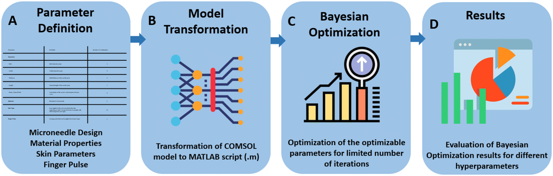
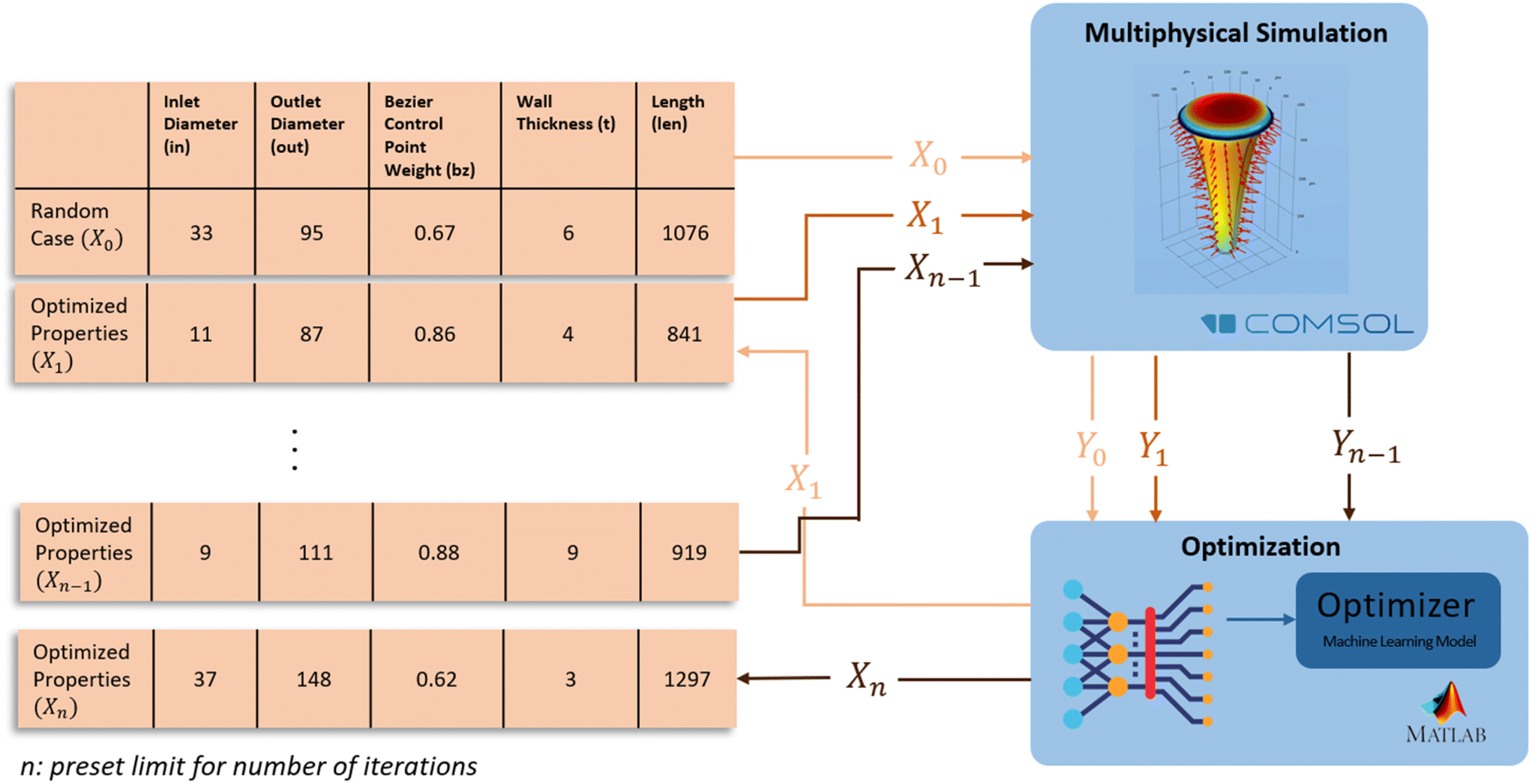
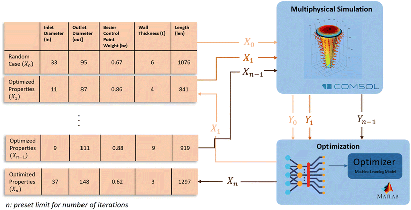
In this work, a computational method was developed to design a microneedle using Bayesian optimization. The method combines the use of a computational model implemented in COMSOL Multiphysics, and the Bayesian optimization algorithm implemented in MATLAB. The optimization process improves the performance of the microneedle in terms of its ability to retract the maximum amount of interstitial fluid (ISF). The optimization was performed on different design parameters including length, inlet diameter, outlet diameter, thickness and parameters of the Bezier curve that defines the curvature of the microneedle. The results of this optimization process provide insight into the optimal design of microneedles for transdermal drug delivery and demonstrate the potential of Bayesian optimization as a powerful tool for optimizing the design of medical devices. Fig. 1 shows the workflow of the research approach.
 |
| | Fig. 1 Workflow of the simulation design. (A) Definition of microneedle parameters that affect overall performance. (B) Transforming the model into a MATLAB function with design parameters as the input and volumetric flow rate (VFR) as the output. (C) Applying Bayesian optimization with the model function as the objective function. (D) Obtaining and verifying the results. | |
2. Methods
2.1 Design parameters
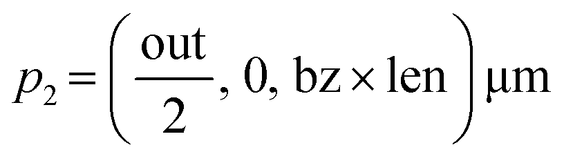
The design parameters for the microneedle model include the length (len), inlet diameter (in), outlet diameter (out) and the wall thickness (t) of the microneedle, and the Bezier curve parameter (bz). For the initial design, length of the microneedle is constant at 30 μm, while the wall thickness is constant at 5 μm. The inlet diameter is constant at 20 μm, and the outlet diameter is constant at 100 μm. The quadratic Bezier curve, which defines the concave profile of the microneedle, is described by three control points:
Bezier curve parameter for the initial design is constant at 0.7. To obtain a 3D model, 2D cross-section of the microneedle as a closed curve with two line segments and two QBCs are revolved with reference to z-axis using COMSOL Revolve function.
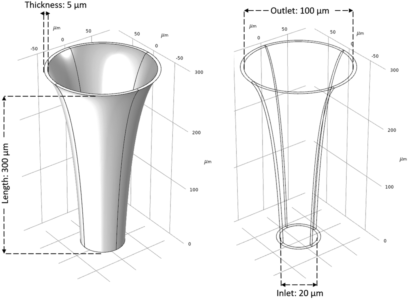
Initial geometrical parameters are based on previous designs.14–17 Similarly, range of parameters are defined within the fabrication limitations for designated materials of the microneedle. When selecting materials for a microneedle matrix to minimize skin swelling or degradation, it is essential to choose biocompatible materials that are well-tolerated by the skin. Some suitable materials for microneedle matrices that have demonstrated biocompatibility and minimized skin reactions include silicon, polymers such as polydimethylsiloxane (PDMS) and polylactic acid (PLA), and metals such as titanium and stainless steel.18–21 Using metals for microneedles can be advantageous due to their excellent mechanical strength and biocompatibility, making them effective for precise and reliable skin penetration during drug delivery or biological fluid sampling. In this study, stainless-steel is chosen as the material for validating the simulations. Parameters len, in, out, and t are defined as integers, while parameter bz is defined as a real number, further discussed in section 2.3. Fig. 2 illustrates the initial design of the MN.
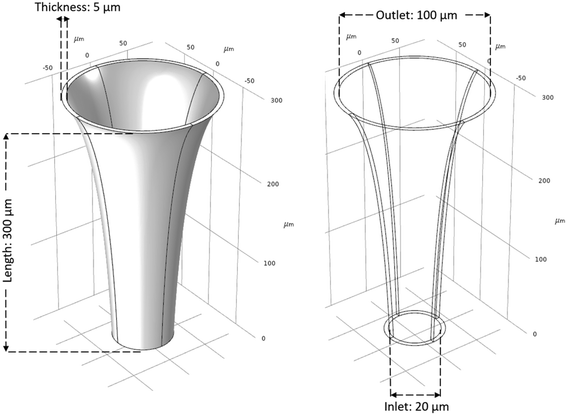 |
| | Fig. 2 Initial design of the MN created in COMSOL Multiphysics. The microneedle has a wall thickness of 3 μm, length of 300 μm, inlet diameter of 20 μm, and outlet diameter of 100 μm. A 2D sketch is drawn as the cross-sectional profile of the MN which consists of two line segments that define the inlet and outlet diameters, and a QBC that defines the curvature of the MN. The 2D sketch is revolved 360 degrees around z-axis in order to create the 3D model of the MN. This design serves as the default mode for the microneedle. | |
2.2 Simulation model
Mechanical CFD simulations were performed in COMSOL Multiphysics®. The model was created using the laminar flow and solid mechanics modules. The fluid flow was modeled using the Navier–Stokes equations for laminar flow in a 2D domain. The fluid was considered to be incompressible and Newtonian, with a dynamic viscosity of 0.001 Pa s. The fluid flow rate was determined by specifying a volume force at the inlet and a no-slip condition at the outlet.
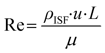
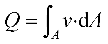
A method was developed to design the optimal microneedle for ISF collection and the fluid parameters were defined accordingly. Reynold's number for the flow in a single MN is defined as:
| |  | (1) |
where
ρISF is the density of ISF (1000 kg m
−3),
22u is the flow velocity (0.001 m s
−1, maximum reported velocity),
L is length of the microneedle (1300 μm), and
μ is the dynamic viscosity of ISF (3.5 × 10
−3 kg m
−1 s
−1).
22 Length is assumed to be at maximum, with the resulting maximum Reynold's number of 10. Thus, the flow is assumed to be laminar.
ISF pressure is within the range of −0.5 mmHg and −8.0 mmHg,23 where the negative sign refers to the “dehydrated state” within the lymph flow.24 ISF pressure is assumed to be 4.0 mmHg (∼530 Pa) and extraction pressure is assumed to be 4.5 kPa based on average human finger pulse.17 Bernoulli's incompressible flow principle states that sum of flow work, kinetic energy, and potential energy of the fluid remains constant throughout a rigid channel25 Bernoulli's equation can be implemented as:
| | 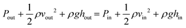 | (2) |
where
P is pressure,
v is flow velocity,
g is the gravitational acceleration,
h is height of elevation and
ρ is fluid mass density for the outlet and any point on
z-axis. Assuming mass is conserved through the microneedle, (
Aout·
vout =
Ain·
vin), volumetric flow rate (VFR) is defined by the cross-sectional area multiplied by flow velocity at any point in
z-axis.
| |  | (3) |
Eqn (4) defines VFR as a function of
r throughout the microneedle, where
A is the cross-sectional area, which is a function of radius, and
v is the velocity of individual points on
z-axis. The model was exported as a MATLAB .m file using LiveLink, which allows for integration with MATLAB.
2.3 Optimization
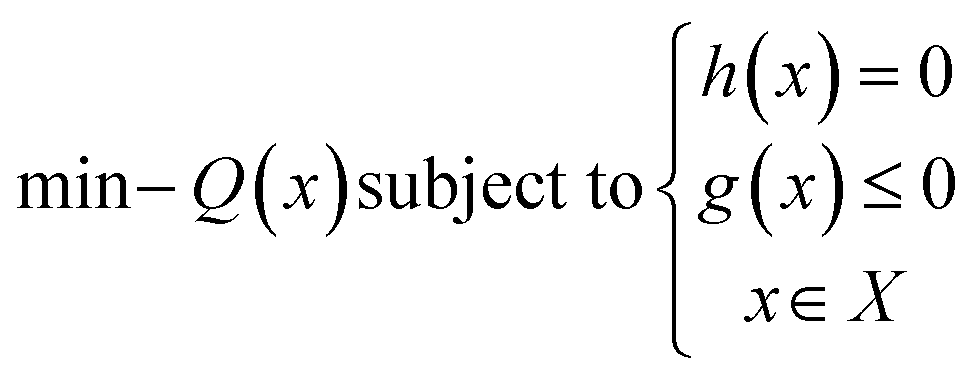
The design of an instrument through optimization involves finding the best design by minimizing an objective function that expresses the problem mathematically, while considering certain limitations or constraints. This type of optimization can lead to improvements in factors such as performance, efficiency, and cost. However, it the relationship between the design's features and its performance is often not straightforward and may require nonlinear programming techniques to properly optimize the design. Nonlinear maximization problem here is mathematically defined as:| |  | (4) |
where Q(x) is the objective function, X is a subset of R5 a.k.a array of geometrical parameters, and h(x) and g(x) are equality and inequality constraints, respectively.
The optimization of the microneedle design was performed using MATLAB's “bayesopt” function. The function is a Bayesian optimization algorithm, which uses a probabilistic model to guide the search for the optimal design parameters. The algorithm takes the design parameters and their corresponding volume flow rate of ISF into account and finds the combination of parameters that gives the maximum volume flow rate. The algorithm begins with a prior distribution on the design parameters, which reflects the initial knowledge about the design space. As the algorithm explores the design space, it updates the prior distribution based on the observed results, to form a posterior distribution that represents the current state of knowledge. The algorithm then uses the posterior distribution to select the next design point to evaluate. The process is repeated until the algorithm converges to an optimal design. Fig. 3 shows the iterative optimization schema with Bayesian optimization.
 |
| | Fig. 3 Workflow of the Bayesian optimization. The algorithm begins by initializing with an initial guess for the microneedle design parameters, incorporating prior knowledge or assumptions. Each iteration intelligently selects a new sample point using an acquisition function, striking a balance between exploring unexplored regions and exploiting promising ones. This iterative process efficiently drives Bayesian optimization towards the optimum. For the selected sample point in each iteration, the objective function, which quantifies the performance metric of interest (VFR), is evaluated. The objective function is evaluated for preset number of n iterations, the sample point that maximizes the VFR is selected as the optimum design configuration. This chosen point represents the most favorable set of design parameters that maximize the desired performance metric. | |
A key feature of Bayesian optimization is the acquisition function, which is used to balance the exploration and exploitation of the design space. The acquisition function gives a measure of the expected improvement at each design point, by considering the uncertainty in the model predictions. Some commonly used acquisition functions include probability of improvement (PI), expected improvement (EI), and upper confidence bound (UCB). Each of them has their own strengths; in this work, EI was used as it is computationally efficient and has proven to be a good general-purpose acquisition function. The optimization process was run multiple times with different iteration numbers to ensure that the global optimum was found. The optimal design parameters were validated by comparing the estimated objective value with the simulation results. The optimization process with Bayesian optimization is a reliable way to find the optimal parameters for a microneedle design to maximize the ISF flow rate. Table 1 shows the upper and lower bounds, and the variable types of the parameters.
Table 1 Upper and lower bounds, and variable types of the parameters
| Parameter |
Lower bound |
Upper bound |
Variable type |
| Length (len) [μm] |
100 |
1300 |
Integer |
| Inlet diameter (in) [μm] |
5 |
40 |
Integer |
| Outlet diameter (out) [μm] |
50 |
150 |
Integer |
| Wall thickness (t) [μm] |
3 |
10 |
Integer |
| Bezier curve parameter (bz) |
0.6 |
0.9 |
Real |
3. Results and discussion
3.1 Optimization results
Bayesian optimization algorithm was run several times for 1500 iterations to determine the optimal number of iterations. After 400 iterations, objective value did not improve further. Thus, the optimal iteration number was determined to be 400 for the model. Hyperparameter optimization using Bayesian optimization in MATLAB involved tuning several key hyperparameters to enhance the optimization process. AcquisitionFunctionName hyperparameter determines the strategy for selecting the next evaluation point. Choosing an appropriate acquisition function influences the exploration–exploitation trade-off, affecting the balance between exploring new regions of the parameter space and exploiting promising regions identified so far. IsObjectiveDeterministic hyperparameter specifies whether the objective function is deterministic or stochastic. A deterministic objective function always produces the same output for a given set of input parameters, while a stochastic objective function introduces randomness. This distinction is crucial for guiding the optimization process effectively. ExplorationRatio hyperparameter controls the propensity to explore unexplored regions of the parameter space. Adjusting this ratio influences the algorithm's willingness to search beyond the known optimal regions, potentially leading to the discovery of better solutions. GPActiveSetSize hyperparameter determines the number of data points used to fit the Gaussian process (GP) model. A smaller GP active set size can accelerate the optimization process by reducing computational complexity, but it may sacrifice accuracy. Balancing this trade-off is essential for achieving efficient optimization while maintaining accurate modeling of the objective function. UseParallel hyperparameter enables or disables parallel computing during the optimization process. Leveraging parallelism can significantly speed up the computation, particularly when the objective function evaluations are time-consuming. MaxObjectiveEvaluations hyperparameter sets the maximum limit for the number of evaluations of the objective function. This constraint allows controlling the computational budget for optimization, preventing excessive evaluations while striving for convergence to the optimal solution. MaxTime hyperparameter defines a time limit for the optimization process. Setting this limit ensures that the optimization terminates within a specified duration, helping to manage computational resources effectively. Lastly, the NumSeedPoints hyperparameter determines the number of initial evaluation points. These points serve as the starting positions for the optimization process, influencing the exploration of the parameter space from the beginning. Tuning these hyperparameters appropriately is crucial for fine-tuning the optimization process, improving convergence speed, balancing exploration and exploitation, managing computational resources efficiently, and achieving optimal solutions in hyperparameter optimization using Bayesian optimization. Table 2 shows the hyperparameters for the optimization algorithm.
Table 2 Hyperparameters of the Bayesian optimization algorithm
| Hyperparameter |
Definition |
Value |
| AcquisitionFunctionName |
Function to choose the next evaluation point |
Expected-improvement-per-second-plus |
| IsObjectiveDeterministic |
Deteministic objective function |
False |
| ExplorationRatio |
Propensity to explore |
0.5 |
| GPActiveSetSize |
Fit Gaussian process model to GPActiveSetSize or fewer points |
300 |
| UseParallel |
Compute in parallel |
False |
| MaxObjectiveEvaluations |
Objective function evaluation limit |
217 |
| MaxTime |
Time limit |
Infinite |
| NumSeedPoints |
Number of initial evaluation points |
4 |
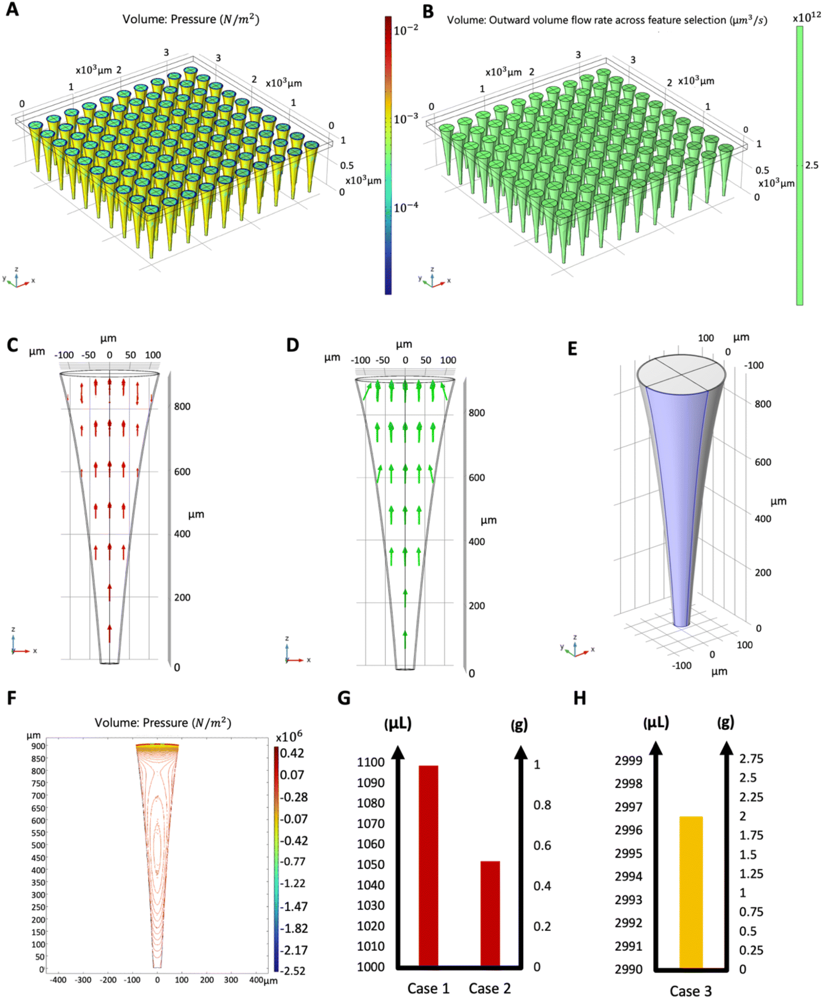
Fig. 4 shows the function evaluations of the Bayesian optimization algorithm. Objective function was defined as negative to transform the optimization problem as a minimization problem. Optimization results were validated by presenting the COMSOL model with the maximizing parameters of the objective function, and it was found that the simulation result matched with the maximum objective value. Fig. 5 shows the simulation results with maximizing parameters of the objective function both as a 10 × 10 array of microneedles as a patch (Fig. 5A and B), and individual microneedles (Fig. 5C and D). Since the microneedle was assumed to be symmetric, pressure distribution was plotted for a single boundary representing the microneedle surface (Fig. 5E and F).
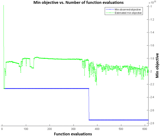 |
| | Fig. 4 Minimum objective value with respect to number of function evaluations. The Bayesian optimization algorithm gradually converges towards the optimal solution, achieving the minimum objective value after approximately 400 iterations. The green lines represent the estimated minimum objective value at each iteration, providing an insight into the algorithm's belief about the optimum. The blue lines depict the observed minimum value of the objective function, reflecting the actual performance achieved during the optimization process. This plot showcases the progressive refinement of the optimization as the algorithm refines its understanding of the problem and seeks to improve the objective function value through iterative exploration and exploitation. | |
 |
| | Fig. 5 COMSOL Multiphysics simulation results for maximizing geometrical parameters. (A) Logarithmic volume pressure difference and (B) outward volume flow rate on microneedles in a patch. (C) Fluid flow and (D) pressure distribution in individual microneedles. Arrow lengths represent relative magnitude. (E) Boundary of the microneedle showing the reference area for (F) contour plot for the pressure distribution on the microneedle surface. Two different fluids, human blood and ISF with various boundary conditions is simulated using the optimal geometry of the microneedle. (G) Amounts of human blood extraction (cases 1 and 2) with the left vertical axis representing the total amount of extracted human blood (μL) and the right vertical axis representing the total amount of extracted human blood (g) over 5 s. (H) Amounts of ISF extraction (case 3) with the left vertical axis representing the total amount of extracted ISF (μL) and the right vertical axis representing the total amount of extracted ISF (g) over 5 s. | |
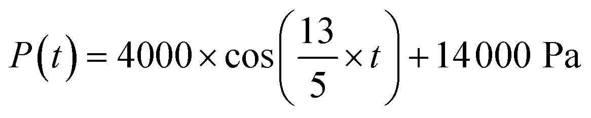
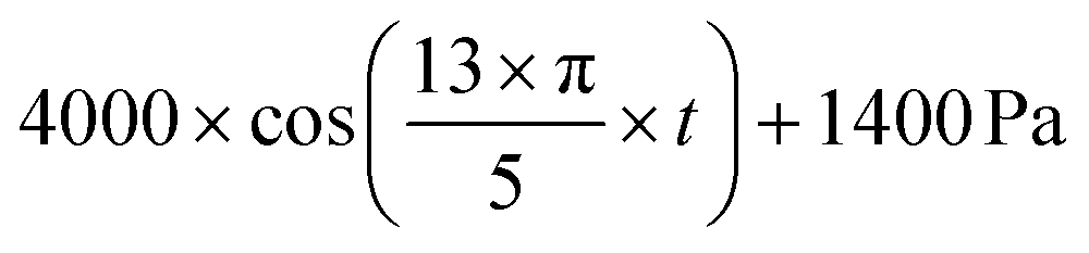
To demonstrate the sample use, 3 different cases were simulated in COMSOL using the optimal microneedle design determined by the algorithm (Table 3). In cases 1 and 2, human blood was assumed to be drawn from the forearm skin using a microneedle array. In case 1, blood pressure was assumed to be constant at 135 mmHg, while in case 2, blood pressure was time-dependent in blood vessels and given by:17
| | 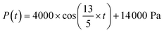 | (5) |
Case 3 was simulated assuming ISF had been drawn from the human forearm with a microneedle array. ISF pressure was assumed to be constant at 4 mmHg.
17 Since density of human blood was substantially higher than ISF, volumetric flow rate was lower.
Fig. 5G and H show that the total amount of fluid extracted from the microneedle array in 5 s for cases 1–2 and 3, respectively.
Table 3 Simulated sample cases for two different target fluids and different inlet boundary conditions
| Case |
Target fluid |
Pressue input |
Fluid inlet pressure |
| 1 |
Human blood |
4500 Pa |
135 mmHg |
| 2 |
Human blood |
4500 Pa |
|
| 3 |
Interstitial luid |
4500 Pa |
4 mmHg |
3.2 Offline vs. online optimization
The optimization of micro/nanofluidic devices has been a widely studied for application in lab-on-a-chip systems and biomedical engineering. Previous studies have approached the design optimization of a microneedle with offline optimization, where an iterative simulation has been performed on COMSOL to obtain a large dataset with parametric sweep.17 Offline optimization requires a significant amount of time to generate a large dataset, which is then used to train ML algorithms to predict the results for an undefined set of parameters.
To overcome the limitations of offline optimization, an online optimization approach was developed in this work. In online optimization, only the initial set of parameters and the bounds were presented to the algorithm, which led to more accurate results with a lower computational load. This approach also allowed for the optimization to be easily adapted to new problem definitions and parameters without the need to create a new dataset, as is the case with offline optimization. Table 4 provides a comparison of offline and online optimization methods.
Table 4 Offline vs. online optimization
| Criterion |
Offline optimization |
Online optimization |
| Maximum run time |
49 h |
17 h |
| Minimum mean squared error |
3.2133 × 10⁻⁶ |
0 |
| Maximum objective value (μL min−1) |
4002 |
16![[thin space (1/6-em)]](https://www.rsc.org/images/entities/char_2009.gif) 502 502 |
In terms of performance, online optimization yielded more accurate results with a higher volumetric flow rate when compared to offline optimization. The optimal parameters for online optimization might change with each run, but the results remained consistently better than those obtained through offline optimization. Additionally, for the same set of parameters, the volumetric flow rate obtained through online optimization was approximately four times higher than that of offline optimization.
4. Conclusion
This study presents an online optimization approach for the design optimization of micro/nanofluidic devices. The developed approach offers several advantages over offline optimization, including lower computational load, greater flexibility in adapting to new problem definitions and parameters, and more accurate results with a higher volumetric flow rate. The results obtained through online optimization demonstrate the potential of this approach for the design optimization of micro/nanofluidic devices in in biomedical applications. Further research could focus on the optimization of other design parameters, such as pressure and temperature, to enhance the performance of microfluidic devices. Simultaneous extraction of blood and ISF could be potentially simulated in our model, yet it would require information about the rheology of blood and ISD (with various mixing ratios). This study shows the development of an optimization method for the design of a microneedle to maximize the volume flow rate of interstitial fluid. The design parameters included the length, inlet diameter, outlet diameter, thickness, and parameters of the Bezier curve that defines the concave profile of the microneedle. The simulation model was created using COMSOL Multiphysics and the Laminar Flow and Solid Mechanics modules, where Navier–Stokes equations were used to model laminar flow in a 2D domain. The optimization was performed using the MATLAB's “bayesopt” function, which is a Bayesian optimization algorithm that iteratively explores the design space to find the optimal combination of parameters. The optimal design parameters were validated by comparing the simulation results to optimization results. The optimization process with Bayesian optimization is a reliable way to find the optimal parameters for a microneedle design to maximize the interstitial fluid flow rate.
Abbreviation
| CFD | Computational fluid dynamics |
| EI | Expected improvement |
| GP | Gaussian process |
| ML | Machine learning |
| MN | Microneedle |
| PDMS | Polydimethylsiloxane |
| PI | Probability of improvement |
| PLA | Polylactic acid |
| UCB | Upper confidence bound |
| VFR | Volumetric flow rate |
Author contributions
CT: conceptualization, software, formal analysis, writing original draft and revise, editing and draft finalizing the manuscript. EA: data handling, software. A. K. Y.: review and editing. ST: supervision, conceptualization, draft editing, finalizing the draft.
Conflicts of interest
There are no conflicts to declare.
Acknowledgements
ST acknowledges TÜBİTAK 2232 International Fellowship for Outstanding Researchers Award (118C391), Alexander von Humboldt Research Fellowship for Experienced Researchers, Marie Skłodowska-Curie Individual Fellowship (101003361), and Royal Academy Newton-Katip Çelebi Transforming Systems Through Partnership award for financial support of this research. Opinions, interpretations, conclusions, and recommendations are those of the author and are not necessarily endorsed by the TÜBİTAK. This work was partially supported by Science Academy's Young Scientist Awards Program (BAGEP), Outstanding Young Scientists Awards (GEBİP), and Bilim Kahramanlari Dernegi The Young Scientist Award. The authors have no other relevant affiliations or financial involvement with any organization or entity with a financial interest in or financial conflict with the subject matter or materials discussed in the manuscript apart from those disclosed. Some elements in Fig. 1 were designed using resources https://flaticon.com.
References
- G. Ma and C. Wu, Microneedle, bio-microneedle and bio-inspired microneedle: A review, J. Controlled Release, 2017, 251, 11–23 CrossRef CAS.
- M. Rezapour Sarabi, S. A. Nakhjavani and S. Tasoglu, 3D-Printed Microneedles for Point-of-Care Biosensing Applications, Micromachines, 2022, 13(7), 1099 CrossRef PubMed.
- S. R. Dabbagh,
et al., 3D-printed microneedles in biomedical applications, iScience, 2021, 24(1), 102012 CrossRef CAS PubMed.
- G. LauraEngelke, SarahHook, JuliaEngerta, Recent insights into cutaneous immunization: How to vaccinate via the skin, Vaccine, 2015, 33(37), 4663–4674 CrossRef PubMed.
- C. Plamadeala,
et al., Bio-inspired microneedle design for efficient drug/vaccine coating, Biomed. Microdevices, 2019, 22(1), 8 CrossRef PubMed.
- A. Jina,
et al., Design, development, and evaluation of a novel microneedle array-based continuous glucose monitor, J. Diabetes Sci. Technol., 2014, 8(3), 483–487 CrossRef CAS PubMed.
- Z. F. Rad, P. D. Prewett and G. J. Davies, Rapid prototyping and customizable microneedle design: Ultra-sharp microneedle fabrication using two-photon polymerization and low-cost micromolding techniques, Manuf. Lett., 2021, 30, 39–43 CrossRef.
- R. F. Donnelly, T. R. Raj Singh and A. D. Woolfson, Microneedle-based drug delivery systems: microfabrication, drug delivery, and safety, Drug Delivery, 2010, 17(4), 187–207 CrossRef CAS PubMed.
- M. R. Sarabi,
et al., 3D printing of microneedle arrays: challenges towards clinical translation, J. 3D Print. Med., 2021, 5(2), 65–70 CrossRef CAS.
- M. Rezapour Sarabi,
et al., Machine Learning-Enabled Prediction of 3D-Printed Microneedle Features, Biosensors, 2022, 12(7), 491 CrossRef CAS PubMed.
- G. Carleo, I. Cirac, K. Cranmer, L. Daudet, M. Schuld, N. Tishby, L. Vogt-Maranto and L. Zdeborová, Machine learning and the physical sciences, Rev. Mod. Phys., 2019, 91(4), 39 CrossRef.
- S. R. Dabbagh,
et al., Machine learning-enabled multiplexed microfluidic sensors, Biomicrofluidics, 2020, 14(6), 061506 CrossRef CAS PubMed.
- S. R. Dabbagh, O. Ozcan and S. Tasoglu, Machine learning-enabled optimization of extrusion-based 3D printing, Methods, 2022, 206, 27–40 CrossRef PubMed.
- B. Ahn, Optimal Microneedle Design for Drug Delivery Based on Insertion Force Experiments with Variable Geometry, Int. J. Control Autom. Syst., 2019, 18, 143–144 CrossRef.
- J. Halder,
et al., Microneedle Array: Applications, Recent Advances, and Clinical Pertinence in Transdermal Drug Delivery, J. Pharm. Innov., 2021, 16(3), 558–565 CrossRef.
- Y. Chen,
et al., A simple and cost-effective approach to fabricate tunable length polymeric microneedle patches for controllable transdermal drug delivery, RSC Adv., 2020, 10(26), 15541–15546 RSC.
- M. R. Sarabi, A. Ahmadpour, A. K. Yetisen and S. Tasoglu, Finger-Actuated Microneedle Array for Sampling Body Fluids, Appl. Sci., 2021, 11, 5329 CrossRef CAS.
- J. W. Lee, M. R. Han and J. H. Park, Polymer microneedles for transdermal drug delivery, J. Drug Targeting, 2013, 21(3), 211–223 CrossRef CAS PubMed.
- H. Nejad, A. Sadeqi and G. Kiaee, Low-cost and cleanroom-free fabrication of microneedles, Microsyst. Nanoeng., 2018, 4, 17073 CrossRef CAS.
- P. Serrano-Castaneda,
et al., Microneedles as Enhancer of Drug Absorption Through the Skin and Applications in Medicine and Cosmetology, J. Pharm. Pharm. Sci., 2018, 21(1), 73–93 CAS.
- X. He,
et al., Microneedle System for Transdermal Drug and Vaccine Delivery: Devices, Safety, and Prospects, Dose-Response, 2019, 17(4), 1559325819878585 CAS.
- W. Yao, Y. Li and G. Ding, Interstitial fluid flow: the mechanical environment of cells and foundation of meridians, Evid. Based Complement. Alternat. Med., 2012, 2012, 853516 Search PubMed.
-
L. M. Ebah, Extraction and analysis of interstitial fluid, and characterisation of the interstitial compartment in kidney disease, PhD, The University of Manchester (United Kingdom): ProQuest, 2012 Search PubMed.
- K. Aukland and R. K. Reed, Interstitial-lymphatic mechanisms in the control of extracellular fluid volume, Physiol. Rev., 1993, 73(1), 1–78 CrossRef CAS PubMed.
- A. Ahmadpour,
et al., Microneedle arrays integrated with microfluidic systems: Emerging applications and fluid flow modeling, Biomicrofluidics, 2023, 17(2), 021501 CrossRef CAS PubMed.
|
| This journal is © The Royal Society of Chemistry 2023 |
Click here to see how this site uses Cookies. View our privacy policy here. 
 Open Access Article
 This Open Access Article is licensed under a
  a,
Erdal
Aydın
a,
Erdal
Aydın