 Open Access Article
Emerging investigator series: a machine learning approach to quantify the impact of meteorology on tropospheric ozone in the inland southern California†
Khanh
Do
 ab,
Manasi
Mahish
c,
Arash Kashfi
Yeganeh
ab,
Ziqi
Gao
d,
Charles L.
Blanchard
e and
Cesunica E.
Ivey
ab,
Manasi
Mahish
c,
Arash Kashfi
Yeganeh
ab,
Ziqi
Gao
d,
Charles L.
Blanchard
e and
Cesunica E.
Ivey
 *abf
*abf
aDepartment of Chemical and Environmental Engineering, University of California Riverside, Riverside, CA, USA. E-mail: iveyc@berkeley.edu
bCenter for Environmental Research and Technology, Riverside, CA, USA
cKenna, Mississauga, Ontario, Canada
dDepartment of Civil and Environmental Engineering, Georgia Institute of Technology, Atlanta, GA, USA
eEnvair, Albany, CA, USA
fNow at Department of Civil and Environmental Engineering, University of California, Berkeley, CA, USA
First published on 15th June 2023
Abstract
The role of meteorology in facilitating the formation and accumulation of ground-level ozone is of great theoretical and practical interest, especially due to changing global climate. In this study, with appropriate machine learning algorithms, we analyzed large meteorology and air quality datasets to train machine learning models to (1) enhance the prediction of ozone levels in the South Coast Air Basin of California, (2) investigate the impact of recent meteorological shifts on ozone formation, and (3) determine the most critical factors influencing ozone exceedance hours. Random forest regression was used to predict historical and future trends of ozone levels, and k-nearest neighbor was used as a binary classifier for ozone exceedance prediction. The models were trained on meteorology data from Ontario and Los Angeles International Airport stations and air quality data from the Fontana, California air monitoring station, and data were collected for the 1994 to 2018 time period. Upon model evaluation, the correlation of the RFR model was 0.92, and the probability of detection for ozone exceedances using k-nearest neighbors was 0.81 for the most recent years of the analysis (2014–2018). We also ran a 4 km Community Multiscale Air Quality model simulation to generate air pollution estimates over Southern California. As expected, ozone in Fontana was positively correlated with temperature. The ozone exceedance hours usually occurred when the temperature was above 25 °C, and the wind direction was from 270° (westerly). Ozone sensitivity as a function of temperature and NOx was also examined. Observed troughs in hourly NOx concentrations during midday under high temperatures suggests that most of the ambient NOx reacted, also as expected. The results indicate that machine learning can support state implementation planning by complementing traditional air quality modeling, reducing simulation time, and exploiting large datasets for historical simulations and future air quality predictions.
Environmental significanceThe South Coast Air Basin of California is one of the most polluted regions in the U.S. and is currently designated as nonattainment for 8 hour ozone. The South Coast Air Quality Management District needs to continue aggressively reducing NOx and VOC emissions to combat the impacts of changing climate (rising temperatures). Multi-decadal analyses of meteorological and air quality data enable scientists and regulators to determine key environmental regimes for peak ozone levels. However, deterministic modeling and analysis can be computationally expensive. In this paper, we find optimal predictive algorithms to determine key meteorological regimes that lead to hourly ozone exceedances. Our methods can be readily applied for any polluted region seeking to understand regulatory attainment challenges due to changing climate. |
1. Introduction
California's South Coast Air Basin (SoCAB) is well-known for its poor air quality due to its unique topography and high anthropogenic emissions. Meteorological variables and synoptic patterns greatly influence air pollution in SoCAB.1,2 Los Angeles' temperature inversions resulting from high-pressure systems over SoCAB combined with a mountain wave-induced downslope flow creates a trap that accumulates air pollutants near the ground, leading to degraded air quality.3,4 The relationship between ozone (O3), its anthropogenic precursors, nitrogen oxides (NOx) and volatile organic compounds (VOC), has been well studied by means of environmental chamber experiments, field studies, and air quality modeling, yet new modeling methods are still needed to better understand why rates of ozone reduction in SoCAB have been lower than previously predicted.5–7 Examining NOx-VOC emission ratios and identifying VOC- and NOx-limited regions are useful practices for creating surface ozone reduction strategies, thereby supporting the development of SoCAB emission-control strategies. Chemical transport modeling is generally considered the most advanced approach for evaluating emission-control strategies, but is subject to uncertainties in emission rates, chemical reaction rates, and meteorological parameterizations. To further understand the quantitative relationship between ambient ozone concentrations and emission precursors, isopleths are developed from observed or modeled data to visualize ozone's sensitivity due to changes in NOx and VOCs.5,8,9In recent years, SoCAB ozone has significantly decreased as a result of emissions control programs implemented by the South Coast Air Quality Management District (SCAQMD), the state of California, and the U.S. EPA. Between 1993 and 2012, NOx and reactive organic gas (ROG) emissions in SoCAB decreased from 1425 to 651 tons per day (tpd) of NOx and from 1522 to 535 tpd of ROGs.10 In response to the reductions, the annual average ozone from 1994 to 2011, only considering hourly concentrations between 10 am and 6 PM, decreased by 12% (64 to 57 ppb) in Riverside, CA.10 To achieve the 0.07 ppm 2015 National Ambient Air Quality Standard (NAAQS) for 8 hour ozone by the attainment deadline of 2037 (Fig. S1 and S2†), SCAQMD proposed further reduction in NOx emissions down to 250 tons per day by 2023 and 200 tons per day by 2031 by shifting from conventional fossil fuel to alternative clean fuels for mobile sources.11 Since 2014, the 8 hour ozone design value for SoCAB has marginally increased despite the continuous reduction in emissions.11 The emissions mitigation has unquestionably improved 8 hour ozone design value over the past several decades. However, it is conjectured that shifts in meteorology have impacted ozone improvements in recent years. Environmental researchers commonly use statistical models (i.e., multiple linear regression, generalized additive models, etc.) to predict changes in ozone concentrations with respect to changes in meteorology and investigate the influence of synoptic and local meteorological parameters on surface ozone concentrations.12–17 The uptick in ozone concentration in recent years despite continued reductions in emissions suggests that meteorological influences should be considered when evaluating the effectiveness of control strategies in locations that are working towards NAAQS attainment. In this paper, we investigate the response of ozone to meteorology in SoCAB over a 25 year period (1994–2018) using new data-driven methods and photochemical modeling. Chemical transport models (CTMs), such as the Community Multiscale Air Quality (CMAQ) model, Goddard Earth Observing System model with atmospheric chemistry (GEOS-Chem), and the Comprehensive Air Quality Model with Extensions (CAMx), are useful tools for air quality researchers to simulate air quality trends and study the sensitivities of air pollutant levels to changes in emissions and meteorology. Although CTMs are relatively precise in representing atmospheric physics and chemical processes, handling the large datasets can be challenging given the limitation of computational efficiency and the complexity of input data. Moreover, CTM software applies complex governing equations to resolve concentrations, and most CTMs are designed for use solely with central processing units (CPUs) to carry out the simulations.
In contrast with CTMs, which solve mathematical equations to estimate the outputs, machine learning uses data to discover underlying patterns or substitute functions that mimic complex mathematical functions. CTM processes can also be optimized with modern hardware, such as graphical processing units, to reduce computation time while retaining the results' integrity.18 Presently, with many air monitoring stations across the U.S., air quality datasets are available with high temporal resolution (hourly data). Our study utilizes machine learning and air quality datasets to identify the pattern of the natural processes and explores the links between meteorology and ozone concentrations, leveraging empirical models and observational data. Previous work has been done to forecast air pollutant exceedances using supervised machine learning algorithms. For example, ozone levels have been predicted with reasonable accuracy using a feedforward neural network.19,20 Further, Hájek et al. (2012) presented a different approach for ozone prediction using support vector regression, which showed a significant improvement in the root mean square error (RMSE) compared to neural networks.21
The objective of this study is to explore the role of meteorology in changing ozone concentrations and ozone exceedances in SoCAB by leveraging results of machine learning and CMAQ. We investigate meteorology-ozone sensitivity by applying machine learning to predict ozone concentrations in Fontana, California (inland Southern California) using meteorological inputs for Los Angeles and Ontario, California. The two meteorological sites represent distinct conditions due to their proximity to or distance from the Pacific Ocean. The machine learning results are analyzed against CMAQ simulations and observational data to evaluate the model performance and explore the common findings between the two approaches.
2. Study location and measurements
The California study sites include Los Angeles International Airport (LAX) and Ontario International Airport (ONT) meteorological sites and the Fontana air quality monitoring site (Fig. 1). LAX is an upwind urban center near the coast of the Pacific Ocean, and use of LAX meteorology enables us to investigate the sensitivity of ozone concentrations at the downwind air monitoring site with respect to upwind conditions. The temperature at LAX in the summer is lower and relative humidity is higher than the other two sites. The meteorology in ONT and Fontana is very similar because they are both in inland Southern California and are located seven miles apart, and they are approximately 50 miles from LAX. In 2018, LAX's annual average temperature was 1.0 °C lower than ONT (17.9 °C for LAX and 18.9 °C for ONT). During the 2010 to 2019 period, the 8 hour ozone design value concentration for LAX fluctuated around 80 ppb, whereas the value for Fontana was consistently above 100 ppb (Fig. S1 and S2†).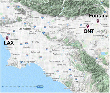 | ||
| Fig. 1 Site location map highlighting the Los Angeles (LAX) and Ontario (ONT) International Airports and the Fontana air monitoring site. | ||
3. Methods
The machine learning (ML) models presented in this paper were trained on Fontana air quality data with both LAX and ONT meteorological data. The models were evaluated using data from the Fontana air monitoring station. The ML models enabled the examination of the relationship between meteorology at any location (e.g., ONT/LAX) and Fontana's air quality. We also carried out a CMAQ simulation with 4 km horizontal spacing for the 2017 ozone season (May 1–Sep 30) in SoCAB, which provided a comparison dataset based on a deterministic model. We describe these methods in detail below.3.1. Data processing
Meteorology and air quality datasets were obtained from the NOAA Climate Data Office and EPA Air Quality System (AQS) database, respectively. The AQS database provides air quality measurements for all valid EPA air monitoring sites in the United States. The meteorology datasets comprised multiple years of observations at LAX and ONT. Meteorological data were obtained for the years 1994 through 2018. Some AQS measurements were made using different samplers; therefore, to ensure uniformity of the data, we selected records from the same instrument whenever possible. Days where data were missing were marked as “NA.” We temporally synced the data from different locations based on their hourly, local timestamp. We randomly selected 80 percent of the data from every year to create a training set, and the remaining 20 percent was used for ML model testing and evaluation.3.2. Machine learning overview
We explored multiple regression-based ML algorithms (e.g., neural network, support vector machine, k-nearest neighbors (K-NN), random forest) by training the models with processed air quality and meteorology data and evaluating predicted ozone concentrations. We mainly focus on the RFR evaluation in this study, as its prediction of ozone concentrations is more accurate for SoCAB. Next, we used binary classification to assign an ozone exceedance label when the observed and predicted hourly ozone concentrations are greater than 70 ppb. Further, we tested different classification methods (e.g., support vector machine, logistic classification, perceptron) to choose the most suitable model for SoCAB.The main difference between classification and regression is in the input and output. The output of classification of any input vector comes from a finite dictionary y ∈ {1,…,m}, where y can be one of the m entries. In this study, the binary classification labels are exceedances and non-exceedances (m = 2) and the output, y can be either exceedances (labeled as 1) or non-exceedances (labeled as 0), whereas in regression, the output can be a real value number, y ∈ R. For regression, the input and output data are provided during training to build a function that correctly predicts the outputs for independent input data that were not used for training.
3.3. Random forest regression
Random forest regression (RFR) is a tree-based ensemble method, and each tree is trained on an independent collection of random input variables. In our study, we defined our vector as X = (Xi,…,Xn)T where n is the number of X features. We wish to find a function f(x) for predicting the ozone concentration, Y. For a random forest of J trees, assuming the decision trees are split into j branches h1(x)…,hj(x), the learning function computes the average from all decision trees, . Thus, the final prediction is based on the average of all outputs from the regression trees.22,23
Due to the nature of regression trees, RFR decision trees can have similarities in tree structures. Shown in Fig. S3† is a three-node decision tree that assists RFR with predicting hourly ozone concentrations (between 12:00 noon and 5:00 PM) based on nitric oxide (NO) and nitrogen dioxide (NO2) concentration and temperature. If a collection of trees in the RF has similar features, the model results are largely biased. To avoid a high correlation in their predictions, the RFR develops the algorithm such that predictions in their subtrees are less correlated by only allowing the trees to have access to a limited number of random samples from a pool of features.24,25 The features we used in our RFR model are temperature (T), relative humidity (RH), surface pressure (P), wind speed (WS), wind direction (WD), visibility (Vis), dewpoint temperature (DT), NO, and NO2, with hourly ozone (O3) as the target variable. To reduce bias, RFR selects a random number of features, and the maximum number of features is defined by the user. Since the concentration of ozone largely depends on precursor emissions and surface meteorology, ML was performed on a predetermined set of meteorological and air quality data to better capture the interactions of meteorology and emissions in an empirical model.26
3.4. RF algorithm tuning (model descriptions)
We used the Python RandomForestRegressor package from the scikit-learn 0.22 library. RFR was tuned with multiple configurations to choose the appropriate set of hyperparameters. Seven hyperparameters were varied to build the RFR model. We used a grid search for multiple combinations resulting in the optimal hyperparameters for the most accurate predictions. Fig. 2 shows the mean absolute error (MAE) in ozone prediction when the RFR model is tuned with various configurations. For example, to find the best fit for the n_estimators parameter, we hold constant values for the other options (e.g., max_features = ‘auto’, max_depth = None, min_samples_split = 5, and min_samples_leaf = 10) and vary n_estimators from 1 to 100. The results show the improvement of the trained model as the number of trees increases. However, when n_estimators approaches 16, the model shows no improvement in the overall performance. Based on the tuning exercise, we picked the optimal values for each hyperparameter that returned the lowest MAE. Our optimal configurations are also informed by the scikit-learn documentation.27 Further, while splitting each node during decision tree building, RFR picks the best split from our nine input features or a random subset of max_features (Table 1). Each tree is trained on a randomly drawn bootstrap sample with replacement from the original training dataset.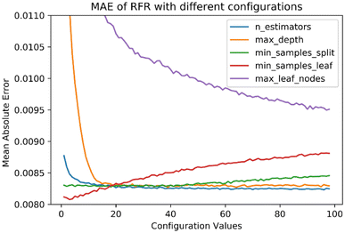 | ||
| Fig. 2 RFR mean absolute error (MAE) with different hyperparameter values. The value of the tuning parameter was varied from 1 to 100 while keeping others constant. MAE is in units of ppm. | ||
| Hyperparameter | Description |
|---|---|
| n_estimators = 16 | The number of trees in the forest |
| max_features = ‘auto’ | The number of features to consider when looking for the best split |
| max_depth = none | The maximum depth of the tree |
| min_samples_split = 5 | The minimum number of samples required to split an internal node |
| min_samples_leaf = 30 | The minimum number of samples required to be at a leaf node |
| min_weight_fraction_leaf = 0 | The minimum weighted fraction of the sum total of weights required to be at a leaf node |
| max_leaf_nodes = none | Best nodes are defined as relative reduction in impurity |
| n_jobs = 8 | The number of jobs to run in parallel |
3.5. K-nearest neighbor classifier
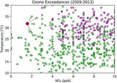
For any given prediction, the model needs to find the closest sample in the training dataset and assign its classification to the prediction label. There is no learned model for K-NN, and the algorithm has to search the entire training set for every test vector.28Fig. 3 shows a binary classification in two dimensions with NO2 on the x-axis and temperature on the y-axis. The green dots are non-exceedances, the purple dots are exceedances, and the red dot is the datum needing to be classified. If k is 5, for example, K-NN searches throughout the training dataset to choose five closest data points and assigns the label by the majority vote amongst the 5 nearest neighbors. Selecting the correct nearest neighbor is crucial to train this model successfully. The model is overfitted when k is small and underfitted when k is large. By varying k from 1 to 8000 and keeping other parameters constant, we can find the optimum k that gives the best accuracy and probability of detection for specific K-NN models (Fig. S4†).3.6. Neural network
Other ML methods used in this study are neural network (NN) and support vector machines (SVM). NN is a multilayer perceptron, where each perceptron is a linear transformation followed by a nonlinear activation (e.g., signum, logistic, rectified linear activation function (ReLU)).29 Each perceptron can be expressed as y[k]i = φ(w[k]Tix + b[k]), where the superscript k denotes the nodes of hidden layers, w[k]Tix + b[k]i is a linear combination model, subscript i is the perceptron at layer k, and φ is the nonlinear activation. NN is a deep network architecture with the depth of the network derived from the level of hidden layers.28,30Fig. 4 shows the diagram for a fully connected 2-layer neural network. All the inputs x are connected to every perceptron in the hidden layer. a1[1] is the perceptron 1 in hidden layer 1, which can be expressed as a[1]1 = φ(w[1]T1x + b[1]1). In this paper, we used ReLU as the activation function defined as φ = max(0,(w[1]T1x + b[1]1)). In terms of matrix representation, the output of the 1st hidden layer is y[1] = φ(W[1]x + b[1]), and the output layer is ŷ = φ(W[2]y[1] + b[2]). We want to find the weights W[1] and W[2] that give the best prediction. In general, for multi-layer neural network the output can be expressed as ŷ = wTφ(W[L]φ(W[L−1]…φ(W[2]φ(W[1]x)))), where w is the weight of the final layer. After computing the predicted output ŷ, the loss function is used to evaluate the difference between the predictions and actual values, L(W) = l(y,ŷ). The gradient descent is used to update the weight, w to obtain better predictions for the next iterations. The process repeats with the new updated w until the loss no further substantially decreases.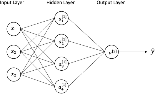 | ||
| Fig. 4 A fully connected 2-layer neural network diagram with inputs x, four perceptrons in the hidden layer, and one in the output layer. | ||
3.7. Support vector machines
SVM is a learning algorithm that optimizes a hyperplane to maximize the margin between different data types. The property required for SVM is to find the supporting hyperplanes and maximize the gap between them.28,31Fig. 5 shows the separating hyperplane (solid line) in the center of the two supporting hyperplanes (dash lines) that maximize the margin between the black dots and white dots. The supporting hyperplanes can be expressed as wTx + b = c for black dots and wTx + b = −c for the white dots, where w is the weight, x is the input, b is the bias, and c is the arbitrary distance which can be set to 1. The distance between two supporting hyperplanes can be maximized by solving the optimization problem, as follows:
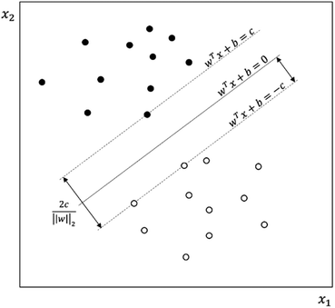 | ||
| Fig. 5 Support vector machine separating black dots and white dots. The separating hyperplane (solid line) is in the center of the two supporting hyperplanes for which the margin is maximized. | ||
3.8. CMAQ model descriptions
We implemented CMAQ version 5.2.1, as the CMAQ model is one of the EPA regulatory methods used to develop ozone attainment control strategies in SoCAB. The CMAQ simulation was carried out for the ozone season of 2017 (May-01 to Oct-01) to concurrently examine the trends that are driving NAAQS nonattainment using a first principles model alongside empirical approaches. The details of CMAQ descriptions can be found in the ESI.†3.9. CMAQ model evaluations
We chose nine key monitoring stations in SoCAB to evaluate our CMAQ simulation, and the stations are located in Anaheim, Azusa, Crestline, Fontana, Los Angeles, Pasadena, Redlands, Rubidoux, and San Bernardino, California (Fig. S5†). To evaluate the model, we followed the EPA guidelines32 and computed a set of unbiased metrics.33 The metrics include correlation coefficient (CC), mean bias error, mean absolute error (MAE), root mean square error (RMSE), relative root mean square error, mean normalized bias, mean normalized absolute error, normalized mean bias (NMB), normalized mean absolute error, fractional bias, fractional absolute error, model mean, and observational mean; the formulas are listed in the ESI.† We evaluated the regression algorithms using the intrinsic metrics of linear fit (e.g., R2, slope, and intercept), CC, RMSE, and MAE. We evaluated different classification algorithms based on probability of detection (PoD), accuracy, model error, and failure to predict (eqn (14)–(17) in the ESI†).4. Results
4.1. Machine learning model evaluation
Before choosing RFR as the principal regressor and K-NN as the principal classifier for our ML applications, we evaluated the predictions for a total of five different models using data for the 1994 to 2018 period (Tables 2 and 3). RFR had the best performance out of four models with the highest CC and R2 and the lowest RMSE and MAE. For classifiers, PoD is the model's ability to detect ozone exceedances for exceedance hours only, and accuracy reflects the performance of the prediction for both exceedances and non-exceedances. Both K-NN and perceptron had reasonable evaluation results. Perceptron had a higher PoD but was less accurate and overfitted the data. K-NN was chosen as the principal classifier for our model, as we prioritized model accuracy.| Regressor | CC | Slope | Intercept | R 2 | RMSE | MAE |
|---|---|---|---|---|---|---|
| a The models were trained on nine features from 1994 to 2018. The models were constructed using 80% of data and evaluated using 20% of the data from the 2014–2018 period. The evaluations are in the unit ppm. | ||||||
| RFR | 0.927 | 0.875 | 0.00605 | 0.861 | 0.009 | 0.006 |
| Neural network | 0.860 | 0.807 | 0.00703 | 0.689 | 0.014 | 0.011 |
| SVR | 0.787 | 1.03 | 0.0194 | 0.619 | 0.028 | 0.024 |
| K-NN | 0.921 | 0.869 | 0.00702 | 0.848 | 0.010 | 0.007 |
| Classifier | PoD | Accuracy | Failure to predict |
|---|---|---|---|
| a The models were trained on nine features from 1994 to 2018. The models were constructed using 80% of data and evaluated using 20% of the data from the 2014–2018 period. The evaluations are in the unit ppm. | |||
| SVM | 0.07 | 0.83 | 0.93 |
| Neural network | 0.76 | 0.71 | 0.24 |
| K-NN | 0.81 | 0.71 | 0.19 |
| Perceptron | 0.83 | 0.69 | 0.17 |
We carried out ten-fold cross-validation to further evaluate the skill of the RFR model. First, the data were shuffled randomly and split into ten groups of equal size. Nine groups were chosen to train the model, and one group was used for evaluation; this was repeated such that each group served as the evaluation group one time. We evaluated the model prediction by comparing the slope, intercept, R2, RMSE, and MAE (Table 4). The ten-fold cross-validation gave consistent performance for each testing group (K) and returned the same RMSE and MAE.
| Metrics | K1 | K2 | K3 | K4 | K5 | K6 | K7 | K8 | K8 | K10 |
|---|---|---|---|---|---|---|---|---|---|---|
| Slope | 0.798 | 0.798 | 0.786 | 0.794 | 0.786 | 0.789 | 0.788 | 0.787 | 0.791 | 0.789 |
| Intercept | 0.007 | 0.007 | 0.007 | 0.007 | 0.007 | 0.007 | 0.007 | 0.007 | 0.007 | 0.007 |
| R 2 | 0.768 | 0.769 | 0.767 | 0.763 | 0.773 | 0.759 | 0.765 | 0.765 | 0.763 | 0.764 |
| RMSE | 0.013 | 0.013 | 0.013 | 0.013 | 0.013 | 0.013 | 0.013 | 0.013 | 0.013 | 0.013 |
| MAE | 0.008 | 0.008 | 0.008 | 0.008 | 0.008 | 0.008 | 0.008 | 0.008 | 0.008 | 0.008 |
We also evaluated the performance of the RFR model for five-year time periods, as ozone concentrations exhibited trend changes roughly every five years (Table 5). The model was trained on 80% of hourly data from 12:00 noon to 5:00 PM during the period of 1994 to 2018, and the remaining 20% of the data were used to test the model in five-year increments (e.g., 1994–1998). In the three periods 1994–1998, 2004–2008, and 2009–2013, the NMB values were negative, indicating that the model underestimates by a factor of 1.069, 1.041, and 1.029, respectively. In the other two periods from 1999–2003 and 2014–2018, NMB values were positive, and the model generally overestimated by a factor of 1.002 and 1.003. A small NMB and a consistently high CC above 0.87 suggests the high performance of the model. Therefore, it is recommended that suitable RFR evaluation metrics for ozone are |NMB| ≤1.05 and a CC ≥0.85.
| Year | CC | MB | MAE | RMSE | MNB | MNAE | NMB | NMAE | FB | FAE |
![[M with combining macron]](https://www.rsc.org/images/entities/i_char_004d_0304.gif)
|
ō |
|---|---|---|---|---|---|---|---|---|---|---|---|---|
| 1994–1998 | 0.88 | −0.004 | 0.013 | 0.018 | 0.035 | 0.263 | −0.069 | 0.214 | −0.039 | 0.234 | 0.055 | 0.059 |
| 1999–2003 | 0.882 | 0 | 0.01 | 0.014 | 0.101 | 0.276 | 0.002 | 0.203 | 0.028 | 0.235 | 0.048 | 0.048 |
| 2004–2008 | 0.884 | −0.002 | 0.009 | 0.013 | 0.011 | 0.19 | −0.041 | 0.165 | −0.025 | 0.182 | 0.052 | 0.054 |
| 2009–2013 | 0.884 | −0.002 | 0.008 | 0.011 | −0.009 | 0.147 | −0.029 | 0.142 | −0.024 | 0.15 | 0.055 | 0.057 |
| 2014–2018 | 0.927 | 0 | 0.006 | 0.011 | 0.036 | 0.151 | 0.003 | 0.142 | 0.017 | 0.143 | 0.058 | 0.058 |
4.2. Historical trends with the RFR model
Results here reflect the trained RFR model for the timespan from 12:00 PM to 5:00 PM when ozone concentrations are high. Fig. 7 and 8 show the three most important variables influencing modeled ozone concentrations in Fontana based on a feature importance screening. Ozone exceedances (defined as hourly observations greater than 0.070 ppm) are associated with high temperature, moderate wind speeds, and lower observed NOx (Fig. 6). High temperatures accelerate ozone's photolytic cycle, while moderate wind speeds accommodate mixing and transport of precursor pollutants. Low NOx conditions suggest that during high ozone hours, NOx is depleted due to the rapid atmospheric turnover of NO2. In the presence of sunlight, NO2 is converted to NO and triplet oxygen, where the triplet oxygen reacts with O2 to form O3. The model performance metric R2 was improved when the model was trained on ONT meteorology, which is most representative of Fontana meteorology, reflecting the dependence of model performance on local meteorology.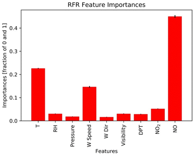 | ||
| Fig. 6 Feature importance generated from the RFR model. NO, T, and wind speed are the three most important features. | ||
 | ||
| Fig. 7 Observational O3 (x-axis) and RFR predictions (y-axis) for Fontana air quality and meteorology from the LAX international airport monitoring station. The plots are for the most recent five-year increment from 2014–2018. The color bars show temperature (a), wind speed (b), and NO (c). Plots for other periods are provided in the ESI.† | ||
 | ||
| Fig. 8 Observational O3 (x-axis) and RFR predictions (y-axis) for Fontana air quality and meteorology from the ONT international airport monitoring station. The plots are for the most recent five-year increment from 2014–2018. The color bars show temperature (a), wind speed (b), and NO (c). Plots for other periods are provided in the ESI.† | ||
Fig. 9 highlights the dynamic application of the RFR model for the 2014–2018 period. Since all-weather elements (e.g., temperature, RH, and surface pressure) are interdependent, varying one strongly affects others. To create the contours, we not only varied temperature and NOx but we also created dynamic pressure and RH arrays by taking the average of the observed RH and pressure at a certain temperature interval. We performed a series of ozone sensitivity tests by continuously feeding desired datasets to the RFR model with varied values of NOx, temperature, temperature-dependent RH, and temperature-dependent pressure while keeping wind speed constant at 9 m s−1. Fig. 9 shows the behavior of ozone with changes in NOx and temperature for four different wind directions (90°, 180°, 270°, and 360°). Ozone concentration reached its maximum at the mid-NOx and high-temperature regime, as predicted by the dynamic RFR model. Ozone significantly decreased as the conditions moved orthogonally in the opposite direction of the high ozone region. Fig. 9d shows that the exceedance usually occurred when NOx concentration was around 10 ppb and the temperature was higher than 35 °C. More than 60% of the time, the wind direction in ONT was from the west, and 25% of the time it was between 254° and 273° (Fig. S6†), which occurred during highest concentration for the region. Ozone concentrations ranged from 0.06 ppm to 0.14 ppm, depending on wind direction. Concentrations were highest when the wind direction was 270° but reached a low for 90° wind direction. The RFR model predicted that the exceedances started to develop at a temperature greater than 30 °C. The ozone concentration gradient (i.e., the change in ozone concentration per unit change in temperature) was small at low temperatures. However, when the temperature approached 30 °C, the gradient became large, and the ozone concentration increased significantly. Ten percent of observed data were plotted on the top of the contour plots in Fig. S7† to validate the observed likelihood of the prediction. The observational data were unevenly spread throughout the domain of the plots. However, the sparseness of observational data was found at the extremely low and high regimes of temperature.
Initially, the RFR model utilized all nine features to predict ozone concentrations. To test ozone prediction sensitivity, the model was trained with nine, eight, seven, and six features after selectively dropping features. The predicted results from each iteration were evaluated against observations using the Wilcoxon rank sum test. If the output from this test was less than or equal to 0.05, two samples were independent of one another, indicating the significance of the dropped feature(s) for the model prediction. The list Wilcoxon tests are shown in Table S1.† The three most important meteorological parameters were wind speed, RH, and temperature as they appeared most frequently in the significant Wilcoxon rank sum tests, suggesting that if they are absent from training features, the RFR model would likely fail to perform with similar accuracy. Also, the two-sample t-test strongly points out that if the three dropped features are RH, wind speed, and temperature or wind speed, NO, and NO2, the model would likely have poor agreement with observations. Table S2† shows three-feature removal combinations where the CC is less than or equal to 0.8.
4.3. Predicting the exceedance hours using K-nearest neighbors
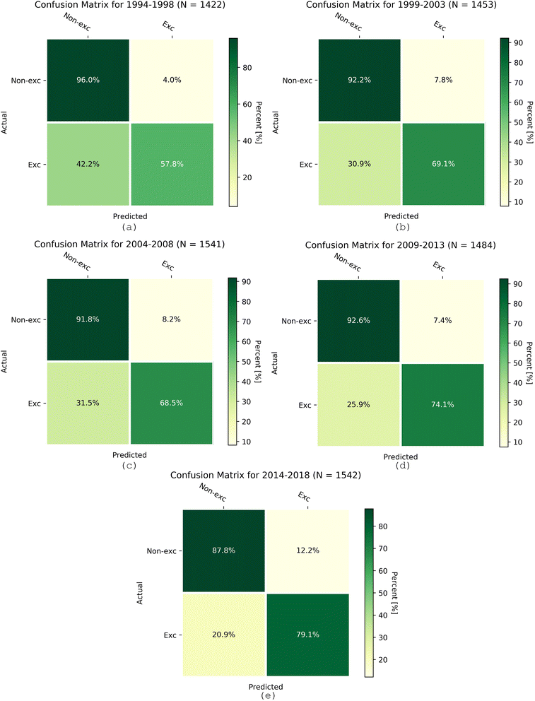
RFR underestimates high ozone concentrations and fails when it comes to extreme ozone levels. The k-nearest neighbor algorithm overcame this barrier when predicting exceedances and proved its accuracy for binary classification (Table 6). We evaluated the K-NN model for 1994–2018 in five-year intervals, similar to the procedure for the RFR model. The PoD of K-NN ranged from 0.58 for the earliest period to 0.81 for the latest period, indicating the improving model performance in later years (Table 6). The accuracy was above 0.71, and only 19% of the time did K-NN not detect the exceedances in the 2014 to 2018 period. Because the dataset was unbalanced due to a higher frequency of non-exceedances, the accuracy yields can be slightly misleading. Even though the model obtained high accuracy, it failed to detect ozone exceedances for up to 42% of the time in earlier years. Fig. 10 shows 2 × 2 confusion matrices for every five years from 1994 to 2018. The dominance of correct non-exceedance prediction (quartile I) and correct exceedance prediction (quartile IV) confirms the overall satisfactory performance of the K-NN model.| Year | PoD | Accuracy | Failure to predict |
|---|---|---|---|
| 1994–1998 | 0.58 | 0.84 | 0.42 |
| 1999–2003 | 0.69 | 0.87 | 0.31 |
| 2004–2008 | 0.69 | 0.86 | 0.31 |
| 2009–2013 | 0.74 | 0.87 | 0.26 |
| 2014–2018 | 0.81 | 0.71 | 0.19 |
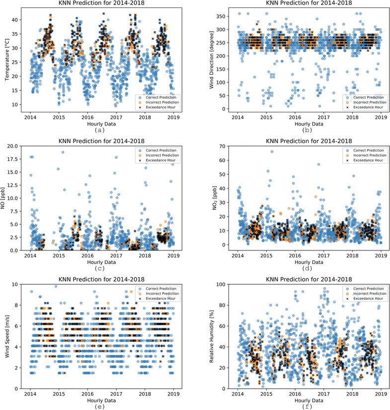
Even though NOx and VOCs are two significant components influencing ozone formation, meteorology is also a crucial driving force. Fig. 11 shows an oscillating pattern of temperature, alternating between winters and summers from 2014–2018 as expected. Below 22 °C, no exceedances occurred, and most exceedances occurred during the summertime. The K-NN model successfully explained the link between temperature and exceedances and accurately predicted the exceedances when the temperature is high and predicted no exceedances when the temperature fell below 22 °C. The exceedances did not usually occur for high NOx, high RH, or low wind speed. As evident in Fig. S7 and S11,† high RH was associated with low temperatures and ozone, and lower NOx concentrations were associated with high temperatures in this analysis. Fig. 11 shows a strong relationship between specific meteorological regimes and exceedance hours. The marine layer penetration on foggy days might cause high RH. During these episodes, the marine layer is deep and moves farther inland with the clean air.
4.4. CMAQ evaluation
The CMAQ simulation provides a deterministic evaluation for comparison with the ML predictions. The daily average ozone concentrations from the 2017 CMAQ simulation were extracted and evaluated against observational data at nine air monitoring sites (Table S5†). Positive MB for all evaluation sites suggest the overall overestimates of the model with a maximum MB of 16 ppb (Fontana) and a minimum of 6 ppb (Crestline and LA). The overestimation occurred because the model did not capture the low ozone concentrations at night (Fig. S8†), which significantly increased the CMAQ daily average ozone concentrations. Since this paper focuses on ML, the details of the comparative CMAQ evaluation can be found in the ESI.†4.5. Methods strengths and limitations
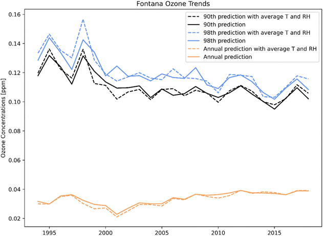
The ML model nimbly predicts the changes of the target variable with respect to a perturbation in input features (i.e., ozone response to changing in temperature). The effect of meteorology can also be determined by examining trends over a long period of time. When using average temperature and RH from 1994 to 2018, the ML prediction minimized the effect of meteorology extremes on ozone formation (i.e., heat waves, foggy days). Fig. 12 shows the annual 90th percentile (blue), annual 98th percentile (black), and the annual average (orange) ozone trends at the Fontana location for 1994 to 2018. The dashed lines are the ML prediction with the average temperature and RH, and the solid lines are the prediction with the actual features. The adjusted line shows a strong downward ozone trend from 1994 to 2010, but resisting further decrease in later years. The distance between the 98th and 90th ozone percentile was narrow, indicating the high frequency of high ozone concentrations in Fontana. The average meteorology had minor effects on the annual average prediction. Despite the downward trend of ozone concentrations for the 90th and 98th percentile, the annual average increased.In contrast with ML, which focused on a targeted pointwise location, CMAQ simulations covered a large spatial domain (102 × 156 grid cells with 4 km spacing) over the South Coast air basin. As expected, model performance is variable when evaluated at specific locations. Despite the less-than-favorable performance at the Fontana location in terms of mean bias error (Table S5†) compared to nine other sites, CMAQ performed better in other locations. Further, Fig. 13 shows monthly spatial evaluations for June and July 2017 for 25 air monitoring sites in SCAQMD, which demonstrates CMAQ's utility in enabling simultaneous detailed examinations of different areas for multiple species, while covering a sizeable spatial area. This paper examines how ML vs. first principles modeling performs for a similar analysis, providing useful insight into the strengths and weaknesses of the methods for the application detailed here.
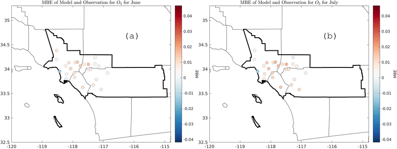 | ||
| Fig. 13 Monthly mean bias error for ozone for 25 air monitoring sites in SoCAB; (a) June 2017, (b) July 2017. | ||
5. Discussion
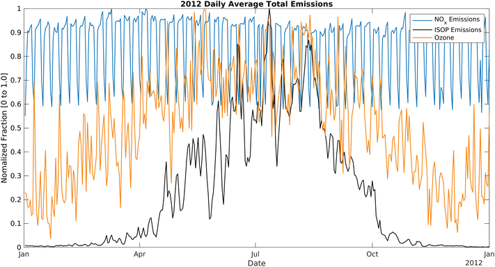
The RFR model was the preferred regressor model for this application. However, the RFR model underestimated high ozone levels and overestimated low ozone levels due to the nature of RFR, in which the model takes the average of all the decision trees. To compensate for this limitation when predicting ozone exceedance hours, we also used binary classifications. The high PoD and accuracy of the K-NN model suggested that K-NN was better suited for ozone exceedance prediction. It can be improved and fine-tuned to achieve better results by optimizing the number of neighbors, leaf size, and the algorithm to compute the nearest neighbors.Evaluation of ML and CMAQ results showed that the temperature was the most significant contributing factor to high ozone concentrations, resulting in spikes of exceedances during the hot summer days. The relationship of temperature with ozone exceedances also varies in different topological regions. Gorai et al., showed that temperature had no uniform correlations and effects on the ozone trend in eastern Texas in May 2012.34 However, in SoCAB, RFR and CMAQ models strongly suggest that temperature is the primary driving force. In the VOC-limited SoCAB35,36 urban area, a reduction in NOx or increase in VOCs may increase ozone formation. During the most severe California drought years (2011–2015), isoprene decreased by more than 50%,37 resulting in a considerable reduction in ozone levels. Fig. 14 and S10† show the daily average emissions of biogenic isoprene and NOx in 2012.11 From January to April, isoprene emissions slowly increase and surpass NOx emissions in May. Emissions remain high throughout the summer and decrease after October. Vegetation emits a large amount of isoprene and other biogenic BVOCs at high temperatures (temperature-dependent isoprene emissions),38 causing an increase in total VOC levels in the summer. NOx emissions during 2012 were roughly constant, with the lows at 130 mol s−1 and the highs at 210 mol s−1 due to the estimated constant contributions from traffic and industrial activities throughout the year. Thus, the high summertime ozone concentration can be partially explained by increased reactions between excess BVOCs emitted from vegetation and NOx, resulting in increased ozone levels in such a VOC-limited regime.
Wind speed and wind direction also influences ozone levels, as shown in the contour plots. Ozone precursors accumulate at low wind speeds, and high ozone levels occur when the wind speed is between 2–4 m s−1. This is optimal wind speed and wind direction to accelerate chemical transport and mixing. More than 64% of the time, the direction of the wind in ONT is from the Los Angeles city center to the east, which transports ozone and precursors to Fontana and further contributes to ground-level ozone formation. High ozone levels occur in the summer when the temperature exceeds 25 °C, and the NOx concentration is low due to the reaction of NO2 with the OH radical.
Results here corroborate the previously demonstrated strong relationship of ozone with meteorology in a data-driven framework. Wind speed and wind direction contribute mainly to transport and mixing of precursors, while the temperature can be a direct contributing factor for catalyzing ozone formation. Climate-related increases in temperature would therefore be expected to increase future ozone levels in the absence of emission changes. The time series from the RFR and CMAQ models shows spikes in temperature that correspond to ozone concentration peaks. Low RH occurs during high-temperature periods, and high RH is observed during low-temperature periods. The predicted effect of RH on ozone level as small, and when RH reached 100%, predicted ozone dramatically decreases.39 RH is a significant feature for ensuring model accuracy based on significance tests.
6. Conclusion
Large, publicly available meteorological databases and open-source libraries (TensorFlow, scikit-learn, and PyTorch) have made ML an efficient and complementary modeling approach for studying long-term air pollution trends, compared to CTMs. We reiterate that CTMs and ML serve different purposes, where CTMs are useful for predicting future pollution levels in response to emission controls. This paper has shown that the RFR and K-NN models were satisfactory for ozone exceedance prediction in SoCAB during the 2017 ozone season. From significance testing and feature importance screening, meteorology data improved model prediction accuracy. In Fontana, ozone exceedances occurred at high temperatures, during periods of lower observed NOx, wind speed above three m s−1, and the RH between 10% and 50%. RFR ML models can be improved by choosing the minimum set of features spanning the tree dependency.40 It is of further interest to create ML models that take input from weather forecasting models to predict ozone concentrations in three dimensions. In future applications, we will tune the configurations on multiple ML algorithms to obtain the most suitable model that accurately predicts ozone exceedances based on meteorology inputs.Conflicts of interest
There are no conflicts of interest to declare.Acknowledgements
The authors thank Prof. Armistead G. Russell and Dr Sang-Mi Lee for their helpful contributions to this work. This paper was prepared as a result of work sponsored, paid for, in whole or in part, by the South Coast Air Quality Management District (SCAQMD). The opinions, findings, conclusions, and recommendations are those of the authors and do not necessarily represent the views of SCAQMD. We acknowledge Graduate Assistant in Areas of Need (GAANN) support from the University of California, Riverside Chemical and Environmental Department.References
- B. L. Ulrickson and C. F. Mass, Numerical Investigation of Mesoscale Circulations over the Los Angeles Basin. Part I: A Verification Study, Mon. Weather Rev., 1990, 118(10), 2138–2161, DOI:10.1175/1520-0493(1990)118<2138:NIOMCO>2.0.CO;2.
- B. L. Ulrickson and C. F. Mass, Numerical Investigation of Mesoscale Circulations over the Los Angeles Basin. Part II: Synoptic Influences and Pollutant Transport, Mon. Weather Rev., 1990, 118(10), 2162–2184, DOI:10.1175/1520-0493(1990)118<2162:NIOMCO>2.0.CO;2.
- R. Lu and R. P. Turco, Air Pollutant Transport in a Coastal Environment-II. Three-Dimensional Simulations over Los Angeles Basin, Atmos. Environ., 1995, 29(13), 1499–1518, DOI:10.1016/1352-2310(95)00015-Q.
- R. Lu and R. P. Turco, Air Pollutant Transport in a Coastal Environment. Part I: Two-Dimensional Simulations of Sea-Breeze and Mountain Effects, J. Atmos. Sci., 1994, 51(15), 2285–2308, DOI:10.1175/1520-0469(1994)051<2285:aptiac>2.0.co;2.
- Y. Qian, L. R. F. Henneman, J. A. Mulholland and A. G. Russell, Empirical Development of Ozone Isopleths: Applications to Los Angeles, Environ. Sci. Technol. Lett., 2019, 6(5), 294–299, DOI:10.1021/acs.estlett.9b00160.
- S. Baidar, R. M. Hardesty, S.-W. Kim, A. O. Langford, H. Oetjen, C. J. Senff, M. Trainer and R. Volkamer, Weakening of the Weekend Ozone Effect over California's South Coast Air Basin, Geophys. Res. Lett., 2015, 42(21), 9457–9464, DOI:10.1002/2015GL066419.
- S. E. Pusede and R. C. Cohen, On the Observed Response of Ozone to NOx and VOC Reactivity Reductions in San Joaquin Valley California 1995–Present, Atmos. Chem. Phys., 2012, 12(18), 8323–8339, DOI:10.5194/acp-12-8323-2012.
- A. Sierra, A. Y. Vanoye and A. Mendoza, Ozone Sensitivity to Its Precursor Emissions in Northeastern Mexico for a Summer Air Pollution Episode, J. Air Waste Manage. Assoc., 2013, 63(10), 1221–1233, DOI:10.1080/10962247.2013.813875.
- J. R. Kinoslan, Ozone-Precursor Relationships from EKMA Diagrams, Environ. Sci. Technol., 1982, 16(12), 880–883, DOI:10.1021/es00106a011.
- F. Lurmann, E. Avol and F. Gilliland, Emissions Reduction Policies and Recent Trends in Southern California’s Ambient Air Quality, J. Air Waste Manage. Assoc., 2015, 65(3), 324–335, DOI:10.1080/10962247.2014.991856.
- South Coast Air Quality Management District, Final 2016 Air Quality Management Plan, 2017 Search PubMed.
- S. C. Kavassalis and J. G. Murphy, Understanding Ozone-Meteorology Correlations: A Role for Dry Deposition, Geophys. Res. Lett., 2017, 44(6), 2922–2931, DOI:10.1002/2016GL071791.
- L. Camalier, W. Cox and P. Dolwick, The Effects of Meteorology on Ozone in Urban Areas and Their Use in Assessing Ozone Trends, Atmos. Environ., 2007, 41(33), 7127–7137, DOI:10.1016/j.atmosenv.2007.04.061.
- N. Otero, J. Sillmann, J. L. Schnell, H. W. Rust and T. Butler, Synoptic and Meteorological Drivers of Extreme Ozone Concentrations over Europe, Environ. Res. Lett., 2016, 11(2) DOI:10.1088/1748-9326/11/2/024005.
- M. W. Gardner and S. R. Dorling, Statistical Surface Ozone Models: An Improved Methodology to Account for Non-Linear Behaviour, Atmos. Environ., 2000, 34(1), 21–34, DOI:10.1016/S1352-2310(99)00359-3.
- S. T. Rao, I. G. Zurbenko and J. B. Flaum, Moderating the Influence of Meteorological Conditions on Ambient Ozone Concentrations, J. Air Waste Manage. Assoc., 1996, 46(1), 35–46, DOI:10.1080/10473289.1996.10467439.
- R. Ooka, M. Khiem, H. Hayami, H. Yoshikado, H. Huang and Y. Kawamoto, Influence of Meteorological Conditions on Summer Ozone Levels in the Central Kanto Area of Japan, Procedia Environ. Sci., 2011, 4, 138–150, DOI:10.1016/j.proenv.2011.03.017.
- C. A. Keller, M. J. Evans, J. N. Kutz and S. Pawson, Machine Learning and Air Quality Modeling, in Proceedings - 2017 IEEE International Conference on Big Data, Big Data 2017, 2018. DOI:10.1109/BigData.2017.8258500.
- G. Corani, Air Quality Prediction in Milan: Feed-Forward Neural Networks, Pruned Neural Networks and Lazy Learning, Ecol. Modell., 2005, 185(2–4), 513–529, DOI:10.1016/j.ecolmodel.2005.01.008.
- H. Xie, F. Ma, Q. Bai, Prediction of Indoor Air Quality Using Artificial Neural Networks, in 5th International Conference on Natural Computation, ICNC 2009, 2009. DOI:10.1109/ICNC.2009.502.
- P. Hájek and V. Olej, Ozone Prediction on the Basis of Neural Networks, Support Vector Regression and Methods with Uncertainty, Ecol. Inform., 2012, 12, 31–42, DOI:10.1016/j.ecoinf.2012.09.001.
- V. Rodriguez-Galiano, M. Sanchez-Castillo, M. Chica-Olmo and M. Chica-Rivas, Machine Learning Predictive Models for Mineral Prospectivity: An Evaluation of Neural Networks, Random Forest, Regression Trees and Support Vector Machines, Ore Geol. Rev., 2015, 71, 804–818, DOI:10.1016/j.oregeorev.2015.01.001.
- C. Zhang and Y. Ma, Ensemble Machine Learning: Methods and Applications, 2012, DOI:10.1007/9781441993267.
- L. Breiman, Random Forests, Machine Learning, 2001, DOI:10.1023/A:1010933404324.
- S. Raschka and V. Mirjalili, Python Machine Learning, 2nd edn, 2006, DOI:10.1037/023990.
- Z. Gao, C. E. Ivey, C. L. Blanchard, K. Do, S.-M. Lee and A. G. Russell, Separating Emissions and Meteorological Impacts on Peak Ozone Concentrations in Southern California Using Generalized Additive Modeling, Environ. Pollut., 2022, 307(119503) DOI:10.1016/j.envpol.2022.119503.
- F. Pedregosa, G. Varoquaux, A. Gramfort, V. Michel, B. Thirion, O. Grisel, M. Blondel, P. Prettenhofer, R. Weiss, V. Dubourg, J. Vanderplas, A. Passos, D. Cournapeau, M. Brucher, M. Perrot and É. Duchesnay, Scikit-Learn: Machine Learning in Python, J. Mach. Learn. Res., 2011, 12(85), 2825–2830 Search PubMed.
- T. Hastie, R. Tibshirani and J. Friedman, Springer Series in Statistics, 2009, DOI:10.1007/b94608.
- S. Sharma, S. Sharma and A. Athaiya, Activation functions in neural networks, Int. J. Appl. Sci. Technol., 2020, 4(12), 310–316, DOI:10.33564/ijeast.2020.v04i12.054.
- X. Wang, A. Kumar, C. R. Shelton and B. M. Wong, Harnessing Deep Neural Networks to Solve Inverse Problems in Quantum Dynamics: Machine-Learned Predictions of Time-Dependent Optimal Control Fields, Phys. Chem. Chem. Phys., 2020, 22(40), 22889–22899, 10.1039/d0cp03694c.
- M. A. Hearst, B. Scholkopf, S. Dumais, E. Osuna and J. Platt, Support Vector Machines, IEEE Intell. Syst. Appl., 1998, 13(4), 18–28, DOI:10.1109/5254.708428.
- Usepa, Guidance on the Development, Evaluation, and Application of Environmental Models, USEPA Publication, 2009 Search PubMed.
- S. Yu, B. Eder, R. Dennis, S.-H. Chu and S. E. Schwartz, New Unbiased Symmetric Metrics for Evaluation of Air Quality Models, Atmos. Sci. Lett., 2006, 7(1), 26–34, DOI:10.1002/asl.125.
- A. K. Gorai, F. Tuluri, P. B. Tchounwou and S. Ambinakudige, Influence of Local Meteorology and NO2 Conditions on Ground-Level Ozone Concentrations in the Eastern Part of Texas, USA, Air Qual., Atmos. Health, 2015, 8, 81–96, DOI:10.1007/s11869-014-0276-5.
- G. Benosa, S. Zhu, M. Kinnon and D. Dabdub, Air Quality Impacts of Implementing Emission Reduction Strategies at Southern California Airports, Atmos. Environ., 2018, 185, 121–127, DOI:10.1016/j.atmosenv.2018.04.048.
- J. M. Heuss, D. F. Kahlbaum and G. T. Wolff, Weekday/Weekend Ozone Differences: What Can We Learn from Them?, J. Air Waste Manage. Assoc., 2003, 53(7), 772–788, DOI:10.1080/10473289.2003.10466227.
- M. A. G. Demetillo, J. F. Anderson, J. A. Geddes, X. Yang, E. Y. Najacht, S. A. Herrera, K. M. Kabasares, A. E. Kotsakis, M. T. Lerdau and S. E. Pusede, Observing Severe Drought Influences on Ozone Air Pollution in California, Environ. Sci. Technol., 2019, 53(9), 4695–4706, DOI:10.1021/acs.est.8b04852.
- J. Coates, K. A. Mar, N. Ojha and T. M. Butler, The Influence of Temperature on Ozone Production under Varying NOx Conditions – A Modelling Study, Atmos. Chem. Phys., 2016, 16(18), 11601–11615, DOI:10.5194/acp-16-11601-2016.
- L. Jia and Y. Xu, Effects of Relative Humidity on Ozone and Secondary Organic Aerosol Formation from the Photooxidation of Benzene and Ethylbenzene, Aerosol Sci. Technol., 2014, 48(1), 1–12, DOI:10.1080/02786826.2013.847269.
- P. Juszczak, D. M. J. Tax, E. Pekalska and R. P. W. Duin, Minimum Spanning Tree Based One-Class Classifier, Neurocomputing, 2009, 72(7–9), 1859–1869, DOI:10.1016/j.neucom.2008.05.003.
Footnote |
| † Electronic supplementary information (ESI) available. See DOI: https://doi.org/10.1039/d2ea00077f |
| This journal is © The Royal Society of Chemistry 2023 |


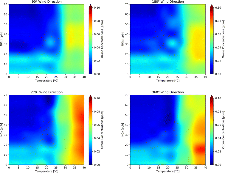
![[thin space (1/6-em)]](https://www.rsc.org/images/entities/char_2009.gif) 000 m), dynamic pressure, dynamic relative humidity, and for four discrete wind directions: (a) 90°, (b) 180°, (c) 270°, and (d) 360°.
000 m), dynamic pressure, dynamic relative humidity, and for four discrete wind directions: (a) 90°, (b) 180°, (c) 270°, and (d) 360°.