DOI:
10.1039/D2LC00303A
(Paper)
Lab Chip, 2022,
22, 3187-3202
Ensemble latent assimilation with deep learning surrogate model: application to drop interaction in a microfluidics device
Received
31st March 2022
, Accepted 1st July 2022
First published on 5th July 2022
Abstract
A major challenge in the field of microfluidics is to predict and control drop interactions. This work develops an image-based data-driven model to forecast drop dynamics based on experiments performed on a microfluidics device. Reduced-order modelling techniques are applied to compress the recorded images into low-dimensional spaces and alleviate the computational cost. Recurrent neural networks are then employed to build a surrogate model of drop interactions by learning the dynamics of compressed variables in the reduced-order space. The surrogate model is integrated with real-time observations using data assimilation. In this paper we developed an ensemble-based latent assimilation algorithm scheme which shows an improvement in terms of accuracy with respect to the previous approaches. This work demonstrates the possibility to create a reliable data-driven model enabling a high fidelity prediction of drop interactions in microfluidics device. The performance of the developed system is evaluated against experimental data (i.e., recorded videos), which are excluded from the training of the surrogate model. The developed scheme is general and can be applied to other dynamical systems.
1 Introduction
Drop microfluidics1–3 is a quickly developing field in science and engineering with multiple applications including foam and emulsion stability,4 processes in colloidal systems and chemical reactions for food5 and biomedical applications,6 enzyme studies,7 cell screening8 and interactions,9 synthesis of catalysts10 and other micro11,12 and nanoparticles.13,14 Drop coalescence is one of the main operations in drop microfluidics. It is widely used to bring reagents together and trigger or quench a reaction or to add additional chemicals/drugs of interest during the cell screening. In these processes, coalescence is a desirable event and 100% coalescence is the aim to be reached. On the other hand, if drops are used as a template for particle formation using various solidification protocols, drop coalescence must be avoided because it results in particle polydispersity. The same is true for foams and emulsions where drop/drop coalescence results in coarsening and ultimate phase separation. These examples show that prediction of drop coalescence in microfluidics and in broader context foam/emulsion stability is of great importance. An additional complexity arises from the presence of reagents inside the drops modifying their viscosity, interfacial tension, and interfacial dynamics. Some surface-active additives can be included in the continuous phase as well. All this together with variability in flow fields and angles at which drops are approaching each other affect coalescence probability.
High-fidelity computational fluid mechanics (CFD) models are frequently used for simulations of micro-scale multi-phase flows. Such interface capture methods as volume of fluid,15 front tracking,16 and level set17 are used for obtaining a sharp interface between phases. However, these methods can incur high computational cost using refined mesh.18 The modelling is especially difficult for the prediction of drop coalescence because of the multiscale character of the problem. This has to be resolved on macroscopic, mesoscopic, and molecular levels taking into account the stochastic character of drop interactions.19 In particular, simulations have to be resolved on a sub-micron length scale accounting for disjoining pressure within the thin liquid film separating drops before coalescence, which is a function of local surfactant concentration, film elasticity due to surfactant redistribution, and thermal fluctuation giving rise to film instability.
In microfluidics, drop coalescence is initiated in different ways: using active methods, such as applied electrical field20 or using passive methods using device geometry, such as coalescence chambers.4,21,22 In the present study, a symmetrical coalescence chamber with two input and two output channels shown in Fig. 1 was used. The flow pattern in this geometry is similar to the compression/extension flow pattern of classical Taylor four-roll mill flow.23 The geometry was successfully used recently for experimental study of drop coalescence in microfluidics.24 In practice, the coalescing drops have different characteristics (e.g. shape, velocity, and relative positions) and it is computationally expensive to use numerical simulation to obtain results for different initial and boundary conditions of interest. Thus, data-driven models based on results of thorough experimental studies with varied flow parameters, drop encounter angles, and chemistry of dispersed and continuous phases are a very promising approach for better understanding and prediction of drop coalescence. Moreover, these models can be further improved by assimilation of numerical data from high-fidelity simulations.
 |
| | Fig. 1 Scheme of the microfluidics device (right): 1 – inlets for dispersed phase, 2 – inlets for continuous phase, 3 – outlet, 4 – X-junctions for drop formation, 5 – coalescence chamber; event of drop coalescence in the coalescence chamber: the processed image and the original image (left). | |
In this work, we aim to predict the dynamics of the microfluidics drop interactions via a data-driven model built from video recordings, combining (ROM) and (DA) approaches. The prediction made by the data-driven model is updated by observed images, which is drawn from the original video with a constant time interval to increase the accuracy of the model output. The process of determining the optimal integration is often referred as DA.25 The assimilation in this study is performed on the latent space (i.e., low-dimensional space), and the approach is named as (LA). In addition, an ensemble-based LA algorithm is proposed in this work to quantify the covariance of prior (prediction) error and determine the optimal assimilation frequency. In this manuscript we show the possibility to create a reliable data-driven model enabling a high fidelity prediction of drop coalescence with the help of some real-time observations. The proposed algorithm scheme consists of two main parts: offline training and online evaluation. The offline part includes the training of ROM and (RNN) while the online part includes the evaluation of surrogate model and real-time DA. The offline part will be of great importance for optimization of microfluidic devices for study of multiple chemical and biochemical reactions, drug, nutrients, flavors and cell encapsulation, and cell screening, including processes where fast precipitation or cross-linking can result in device fouling. In this paper, online DA is used mainly to compensate for the accuracy (which is mainly caused by insufficient training data) of the RNN to further improve the forecasting accuracy.
The rest of the paper is organised as follows, section 2 introduces the related work of machine learning surrogate models for high dimensional dynamical systems. In section 3, the experimental procedures and the backgrounds on the video recorded are covered. The formulation of the data-driven surrogate model and the ensemble-based latent assimilation is presented in section 4. The results of the surrogate model are demonstrated and discussed in section 5. We finish the paper with the conclusion in section 6.
2 Related work and our contributions
Predicting high-dimensional systems in the full physical space can be computationally expensive, if not infeasible.26 To reduce the computational burden, reduced surrogate modelling has been applied on a wide range of dynamical problems, including (CFD),27,28 air pollution modelling29,30 and wildfire prediction.31 It has shown promising results by achieving comparable performance with the high-fidelity models. In the field of ROM, (POD)32 is a well developed concept. It aims to project the full data space to a set of principal directions defined via the empirical covariance matrix. Recent works on fluid mechanics-related problems have been focusing on techniques such as balanced truncation33 and dynamic mode decomposition34,35 to improve the performance of POD approaches. Much effort has also been devoted to determining the optimal truncation parameter of POD-type approaches.36–38 However, the performance of the POD approach can be undermined when building modes from experimental data with incomplete knowledge of the governing equations.39 Extensive research has been done recently to apply (DL) methods in ROM for video anomaly detection, object detection and action recognition.40,41 In these works, the ROM is carried out through DL-based, unsupervised (AE). (CA), a variant of AE with convolutional layers, is extensively employed for compressing image data. Compared to POD, the strength of (ML)-based AEs when dealing with chaotic dynamics has been numerically demonstrated in many engineering problems.42,43 More precisely, CAE have shown its strength in model reduction of laminar flows44 and recently a CAE encoded data-driven model is developed for estimating indoor airflow and ventilation from the numerical simulation results, using DA technique to perform corrections with sensor data.30
Much research effort29,30,45,46 has been given to learn the underlying dynamics in the reduced-order space (also known as the latent space). Among them, the RNNs47 take a sequence of inputs and are generally used to handle time-series prediction. Instead of treating each neuron in parallel as in a traditional (NN) structure. Connections between nodes along temporal sequences can be found in a RNN. When learning long-term dependencies, standard RNN will suffer from problems related to gradients vanishing or exploding48 and it was found that a gated structure can overcome these issues.49 A popular variation, (LSTM),50 contains gated paths that allow the gradients to backpropagate through LSTM units and to avoid gradients vanishing or exploding. There have also been recent reports on applying LSTM-based models to evolve the encoded latent space elements.51,52
Once the prediction using surrogate ML models has been performed, latent data assimilation (also known as latent assimilation (LA))30,53 is employed to adjust the model output on the latent space via real-time observations. DA is widely employed for analyzing model predictions, (also known as background states or a priori estimates) and observations to determine the most probable state (a posteriori estimate). The applications of DA in dynamical systems include field reconstruction and parameters estimation.25 The accuracy of the assimilated results is affected by the modelling of background and observation error covariance matrices.54,55 In theory, the two covariance matrices can be computed by comparing the background state (i.e., model prediction) and the observation to the true state. However, in real DA applications the true state is out of reach, and thus the covariance matrices can only be approximated.56,57 Time-dependent error covariance specification is difficult when applying DA to dynamical systems55 and it impacts crucially the accuracy of DA algorithms.58
Past research on geophysical models has shown that DA frequency has a significant impact on the accuracy of the model59,60 and increasing the DA frequency will not always be beneficial to the prediction accuracy. Too frequent DA increases the computational cost, and it can introduce insertion noise to the model since each DA performed updates the latent variables. Ensemble methods can provide the output distribution and the single-mean prediction. The necessity for correction can be determined by monitoring the Gaussianity of trajectories in the ensemble. Gaussian noises are introduced separately at the start of each trajectory, and an undisturbed trajectory runs in parallel with the ensemble. When the Gaussianity falls below a threshold value, the alert for correction will be raised. The undisturbed trajectory will be corrected with the next observation, and the ensemble will be re-initialized.
In this study, we make use of the National Meteorological Center (NMC)61 method and the ensemble DA approach62 to perform real-time estimation of background covariance inside the latent space where LSTM predictions are performed. The NMC approach, which can also be considered as a variant of ensemble-based DA, was first introduced in meteorological science for efficient background covariance estimation.61 Ensemble-based DA methods such as the ensemble Kalman filter62 or ensemble variational approaches,63 have been widely applied in engineering problems to deal with non-linear dynamical systems. The performances of NMC and ensemble methods are compared with the DA scheme using identity covariance matrices, where the background state and observation contribute equally to the final result. Furthermore, an ensemble-based correction determination algorithm is proposed in this study to investigate the optimum frequency of performing LA.
In general, error covariance specification and correction frequency determination are cumbersome in the reduced space due to the high non-linearity of machine learning functions and the uncertainties generated by the ROM. To overcome these limitations, in the present paper we proposed to integrate ensemble-type methods in the latent assimilation scheme. Numerical results demonstrated that the prediction accuracy can be significantly improved by the proposed approach regarding standard latent assimilation. The adopted method can be applied to various dynamical systems, and we demonstrate its application to drop coalescence in a microfluidics device. In summary, we make the following contributions in this study:
• A (CNN)-LSTM based surrogate model is built with LA for predicting dynamics of a drop pair in a chamber based on microscopic image sequences.
• We propose a novel algorithm that combines the ROM, RNN surrogate models, and ensemble-type assimilation approaches to improve the monitoring of the microfluidic drops in the latent space with real-time observation data. The ensemble methods contribute to both the error covariance specification and the DA frequency determination.
• We compare different ROM approaches, namely POD and CAE in terms of reconstruction accuracy, model prediction performance, and computational time with numerical experiments. The new approach proposed in this work is data-agnostic and can be easily applied to other dynamical systems. The repository of the python code scripts can be found at https://github.com/DL-WG/drop-coalescence-surrogate-model-and-LA.
3 Experiments
The microfluidics device (Fig. 1) used in this study was made of polydimethylsiloxane, PDMS, (SYLGARD 184, Dow Corning) using standard soft lithography technique64 on SU-8 mould. The device was sealed by a glass slide with a spin-coated PDMS layer, using corona discharge treatment and hydrophobized by Aquapel. All channels have a width of 370 μm and a height of 190 μm. The drop diameter in the field of observation was always larger than the channel height, i.e. the drops have a 3D shape of pancakes. The size of the coalescence chamber (distance between the opposite walls) was 862 μm.
The dispersed phase used in this study was an aqueous solution of dodecyl trimethylammonium bromide, C12TAB, (99%, Acros Organics) at concentration 10 mM and continuous phase was silicone oil of viscosity 96 mPa·s (Aldrich). The interfacial tension between continuous and dispersed phases was around 20 mN m−1. The dispersed and continuous phases were supplied by the inlets 1 and 2 (Fig. 1) at flow rates 0.6–1.4 μL min−1 and 3–7 μL min−1 respectively using syringe pumps Al-4000 (World Precision Instruments, dispensing accuracy ± 1%). The ratio of flow rates of the dispersed and continuous phase (per channel) was always kept to 1![[thin space (1/6-em)]](https://www.rsc.org/images/entities/char_2009.gif) :
:![[thin space (1/6-em)]](https://www.rsc.org/images/entities/char_2009.gif) 5. Drops of dispersed phase were formed in two symmetrical flow-focusing cross-junctions 4 and were then transferred by continuous phase to chamber 5 where they meet and then either coalesce or not, and exit the chamber through the symmetrical output channel 3. The parameters affecting coalescence are the total flow rate, the viscosities of the continuous and dispersed phase, the interfacial tension, the presence of surfactant in the continuous or dispersed phase and surfactant properties. The drop size depends on all other parameters and time-lag between the drops arrival to the chamber. In this study, only flow rates and drop lag time were varied whereas all other parameters were kept constant. Drop size was varied slightly (within 5%) due to changes in the flow rate.
5. Drops of dispersed phase were formed in two symmetrical flow-focusing cross-junctions 4 and were then transferred by continuous phase to chamber 5 where they meet and then either coalesce or not, and exit the chamber through the symmetrical output channel 3. The parameters affecting coalescence are the total flow rate, the viscosities of the continuous and dispersed phase, the interfacial tension, the presence of surfactant in the continuous or dispersed phase and surfactant properties. The drop size depends on all other parameters and time-lag between the drops arrival to the chamber. In this study, only flow rates and drop lag time were varied whereas all other parameters were kept constant. Drop size was varied slightly (within 5%) due to changes in the flow rate.
The behavior of the drops from the moment the first of the pair entered the coalescence chamber till the drops were coalesced or separated was recorded using a high-speed video camera (Photron SA-5) connected to an inverted microscope (Nikon Eclipse Ti2-U) at 1000 fps with an exposure of 40 μs using 20× lens which provided a spatial resolution of 1 μm per pixel. The recording was saved as a sequence of TIFF images for further analysis. In total, 49 grey-scale videos were recorded, and each video contains 550 to 600 frames. The observation images were provided to the data-driven surrogate model to perform a correction and to estimate if coalescence will occur in subsequent frames. A frame is periodically extracted (every 60 frames) from the video as the observation yt of time-step t ∈ Tobs where Tobs denotes the time where the observation frame is extracted.
4 Ensemble latent assimilation with deep learning surrogate model
This section presents a data-driven approach that we developed in this paper based on the grey-scale videos recorded from experiments. We first compressed the image data into a low dimensional latent space where two different ROM, namely proper orthogonal decomposition (POD) and convolutional autoencoder, are implemented and analyzed. A recurrent neural network (RNN)-based surrogate model is then trained for predicting drop interactions in the latent space. Finally, we made use of ensemble-based latent assimilation (LA) techniques to perform corrections on the predicted latent variables via synthetic real-time observations.
4.1 Reduced-order-modelling
4.1.1 Proper orthogonal decomposition.
Consider an arbitrary video dataset obtained following the experiments described in section 3, which contains a set of m images with 10242 pixels; for instance, an image at time step t is denoted as xt ∈ ![[Doublestruck R]](https://www.rsc.org/images/entities/i_char_e175.gif) 1024×1024. The video (image dataset) can then be denoted as a matrix X = [xt1,
1024×1024. The video (image dataset) can then be denoted as a matrix X = [xt1,![[thin space (1/6-em)]](https://www.rsc.org/images/entities/char_2009.gif) ⋯xtm] ∈
⋯xtm] ∈ ![[Doublestruck R]](https://www.rsc.org/images/entities/i_char_e175.gif) 1024×1024×m. For applying the vectorwise POD algorithm, state vectors xt will be flattened into (1D) vectors in the rest of sec. 4.1.1, where the new dimensions are xtM ∈
1024×1024×m. For applying the vectorwise POD algorithm, state vectors xt will be flattened into (1D) vectors in the rest of sec. 4.1.1, where the new dimensions are xtM ∈ ![[Doublestruck R]](https://www.rsc.org/images/entities/i_char_e175.gif) 10242, X = ∈
10242, X = ∈ ![[Doublestruck R]](https://www.rsc.org/images/entities/i_char_e175.gif) 10242×m. The image set matrix can be projected to a low-dimensional latent space via (SVD):
10242×m. The image set matrix can be projected to a low-dimensional latent space via (SVD):| |  | (1) |
where r is the rank of X, U = [u1![[thin space (1/6-em)]](https://www.rsc.org/images/entities/char_2009.gif) u2⋯ur] ∈
u2⋯ur] ∈ ![[Doublestruck R]](https://www.rsc.org/images/entities/i_char_e175.gif) 10242×r, Σ ∈
10242×r, Σ ∈ ![[Doublestruck R]](https://www.rsc.org/images/entities/i_char_e175.gif) r×r is a diagonal matrix with positive entries, σ1, σ2, ⋯, σr, and V = [v1v2⋯vr] ∈
r×r is a diagonal matrix with positive entries, σ1, σ2, ⋯, σr, and V = [v1v2⋯vr] ∈ ![[Doublestruck R]](https://www.rsc.org/images/entities/i_char_e175.gif) m×r. The columns of U and V are orthonormal such thatwhere Ir×r denotes the identity matrix of dimension r. The modes uj are the sub-representation of dynamics, while the corresponding diagonal values σj quantify the significance of these modes in the dataset. Denoting the truncation parameter as d, the new truncated modes matrix Ud = [u1u2⋯ud] aims to optimally represent the data with a minimum loss of the variance. The POD encoded image set,
m×r. The columns of U and V are orthonormal such thatwhere Ir×r denotes the identity matrix of dimension r. The modes uj are the sub-representation of dynamics, while the corresponding diagonal values σj quantify the significance of these modes in the dataset. Denoting the truncation parameter as d, the new truncated modes matrix Ud = [u1u2⋯ud] aims to optimally represent the data with a minimum loss of the variance. The POD encoded image set, ![[X with combining tilde]](https://www.rsc.org/images/entities/b_i_char_0058_0303.gif) = [
= [![[x with combining tilde]](https://www.rsc.org/images/entities/b_i_char_0078_0303.gif) t1,
t1,![[thin space (1/6-em)]](https://www.rsc.org/images/entities/char_2009.gif) ⋯
⋯![[x with combining tilde]](https://www.rsc.org/images/entities/b_i_char_0078_0303.gif) tm] ∈
tm] ∈ ![[Doublestruck R]](https://www.rsc.org/images/entities/i_char_e175.gif) d×m can be calculated from:
d×m can be calculated from:| | ![[X with combining tilde]](https://www.rsc.org/images/entities/b_i_char_0058_0303.gif) = UTdX, and = UTdX, and ![[x with combining tilde]](https://www.rsc.org/images/entities/b_i_char_0078_0303.gif) t = UTdxt t = UTdxt | (3) |
From the orthonormal property, the reconstructed image set can be calculated as:where Z, zt denote the decoded image set and the decoded image at time t, respectively. The loss function is computed by the MSE of the image set and the decoded image set, the reconstructed values are capped between 0 and 1 to restrict spurious error caused by reconstruction. The number of modes in Ud has a negative correlation with the calculated MSE, and the total energy proportion contained in the truncated modes matrix Ud can be expressed as| |  | (5) |
Ideally, E will have a value approximate to 1 for high precision data compression. The POD method serves as a benchmark in this work and we compute another data compression strategy based on CAE with the same dimension of the latent space in section 4.1.2.
4.1.2 Convolutional autoencoder.
A typical AE structure is formed with an encoder and decoder, the encoder maps the input data xt to latent variables, ![[x with combining tilde]](https://www.rsc.org/images/entities/b_i_char_0078_0303.gif) t. The fully connected (dense) layers in AE work well with small-scale problems (∼103 degrees of freedom,65,66) but has trouble handling problems characterised by higher degrees of freedom (e.g. 106–109).67 CAE is adopted in this work to exploit the spatial neighbouring correlations.
t. The fully connected (dense) layers in AE work well with small-scale problems (∼103 degrees of freedom,65,66) but has trouble handling problems characterised by higher degrees of freedom (e.g. 106–109).67 CAE is adopted in this work to exploit the spatial neighbouring correlations.
Similar to the encoding-decoding structure of AE, CAE contains upsampling, downsampling, convolutional, and dense layers. The convolutional layers in CAE convolve the input xt ∈ ![[Doublestruck R]](https://www.rsc.org/images/entities/i_char_e175.gif) 1024×1024 with filters (kernels) to generate feature maps by trainable weights. For Nk kernel in a convolutional layer with filter KNk ∈
1024×1024 with filters (kernels) to generate feature maps by trainable weights. For Nk kernel in a convolutional layer with filter KNk ∈ ![[Doublestruck R]](https://www.rsc.org/images/entities/i_char_e175.gif) a×b and filter size (a × b), an element located at (i, j) in the corresponding generated feature map (x * KNk) can be expressed as:
a×b and filter size (a × b), an element located at (i, j) in the corresponding generated feature map (x * KNk) can be expressed as:
| |  | (6) |
where the * denotes the convolution operation. A stride size of
s = 1 is employed here which denotes the number of elements that the filters shifted, from left to right and from top to bottom. The neurons in a convolutional layer can share the same filter: this parameter sharing approach reduces the trainable weight parameters compared to dense layer. The encoder in the CAE is built with a series of convolution max-pooling blocks while the decoder is constructed with a series of convolution-up sampling blocks. The constructed CAE is illustrated in
Fig. 2; the max-pooling and up-sampling are techniques to down-sample and to up-sample feature maps by taking the maximum value and repeating the value, respectively. The input image
xt will be compressed by the encoder, and the encoded image in the latent space is denoted as
![[x with combining tilde]](https://www.rsc.org/images/entities/b_i_char_0078_0303.gif) t
t.
 |
| | Fig. 2 Encoding-decoding layout of the constructed CAE. | |
The encoding and the decoding process can be expressed as:
| | ![[x with combining tilde]](https://www.rsc.org/images/entities/b_i_char_0078_0303.gif) t = t = ![[scr E, script letter E]](https://www.rsc.org/images/entities/i_char_e140.gif) (xt, (xt,![[thin space (1/6-em)]](https://www.rsc.org/images/entities/char_2009.gif) ΘE), zt = ΘE), zt = ![[scr D, script letter D]](https://www.rsc.org/images/entities/i_char_e523.gif) ( (![[x with combining tilde]](https://www.rsc.org/images/entities/b_i_char_0078_0303.gif) t, t,![[thin space (1/6-em)]](https://www.rsc.org/images/entities/char_2009.gif) ΘD) ΘD) | (7) |
where
![[scr E, script letter E]](https://www.rsc.org/images/entities/char_e140.gif)
:
![[Doublestruck R]](https://www.rsc.org/images/entities/i_char_e175.gif) 1024×1024
1024×1024 →
![[Doublestruck R]](https://www.rsc.org/images/entities/i_char_e175.gif) NLS
NLS,
![[scr D, script letter D]](https://www.rsc.org/images/entities/i_char_e523.gif)
:
![[Doublestruck R]](https://www.rsc.org/images/entities/i_char_e175.gif) NLS
NLS →
![[Doublestruck R]](https://www.rsc.org/images/entities/i_char_e175.gif) 1024×1024
1024×1024 denote the encoder and the decoder, which are parameterized by
ΘE and
ΘD, respectively, and
NLS denotes the dimension of the latent space.
The performance of the CAE is evaluated using the MSE of regarding the true and the decoded image set, and the optimal parameters,  and
and  are determined from the binary cross-entropy loss function
| |  | (8) |
where ⊙ represents the Hadamard product,
1 ∈
![[Doublestruck R]](https://www.rsc.org/images/entities/i_char_e175.gif) 1024×1024
1024×1024 denotes the matrix of ones. In this work, cross-entropy is employed as loss function instead of MSE or MAE because of the data imbalance, that is, the drop interface only represents a small number of pixels in each image. Using MSE or MAE as loss function will lead to predictions of blank images. The values of the reconstructed matrix are normalized between 0 and 1 to bound the predicted values. Using the optimal hyperparameters determined from the parameter tuning dataset, the CAE is implemented in Keras and a detailed structure of the selected hyperparameters of the CAE is shown in
Table 1, where ReLU denotes rectified linear unit. The CAE is trained with the gradient-based optimizer,
Adam,
68 with a learning rate of 5 × 10
−5, 5000 epochs, and the loss is computed using binary cross-entropy due to the imbalance in grey-scale pixels. The hyperparamter tuning concerning the structure of the CAE is latter displayed in section 5. The dimension of the latent space, 16, is selected based on the optimal latent space dimension to image matrix size ratio (5.2 × 10
−5) proposed in ref.
30, and the structure of the coalescence chamber, where only around half of the space in images is occupied by the actual chamber.
Table 1 CAE structure used for data compression
| Layer (filter size) |
Kernel size |
Output shape |
Act. |
| Encoder |
| Input |
|
(1024, 1024, 1) |
|
| Conv 2D (8) |
(16, 16) |
(1024, 1024, 8) |
ReLU |
| MaxPooling 2D |
(8,8) |
(128, 128, 8) |
|
| Conv 2D (16) |
(8, 8) |
(128, 128, 16) |
ReLU |
| MaxPooling 2D |
(8, 8) |
(16, 16, 16) |
|
| Conv 2D (32) |
(4, 4) |
(16, 16, 32) |
ReLU |
| MaxPooling 2D |
(4, 4) |
(4, 4, 32) |
|
| Flatten |
|
512 |
|
| Dense |
|
16 |
|
| Decoder |
| Input |
|
16 |
|
| Dense |
|
512 |
|
| Reshape |
|
4, 4, 32 |
|
| Conv 2D (32) |
(4, 4) |
(16, 16, 32) |
ReLU |
| Upsampling 2D |
(4, 4) |
(16, 16, 32) |
|
| Conv 2D (16) |
(8, 8) |
(16, 16, 16) |
ReLU |
| Upsampling 2D |
(8, 8) |
(128, 128, 16) |
|
| Conv 2D (8) |
(16, 16) |
(128, 128, 8) |
ReLU |
| Upsampling 2D |
(8, 8) |
(1024, 1024, 8) |
|
| Conv 2D (1) |
(16, 16) |
(1024, 1024, 1) |
Sigmoid |
Each frame of the recorded video has 1024 × 1024 pixels with a single channel normalized to values between 0 and 1, differences in brightness of each video are addressed by sampling at the corners of videos and scaling linearly, a sample of the processed image is shown in Fig. 1. Different velocities can be reflected from the distances that the drops moved between each frame, thus enabling a purely data-driven approach. A video is randomly selected as the parameter tuning dataset and it is assumed the set can reflect the characteristic of other videos. As for the test dataset, 8 videos are picked randomly from combinations of velocities, coalescence and non-coalescence. Additionally, not all images in the training dataset are used for training CAE, as utilizing the full train dataset will exceed the GPU's memory limit. The training dataset is firstly partitioned, where 66.7% of images are kept for training, the images are deselected following a regular pattern, where an image is removed from the CAE's training dataset for every 3 images in a row. The remaining images are then divided to CAE's training and validation datasets, where validation consists of 20% of the images and they are selected in a similar way as before. Same measures are applied for determining the parameters of POD.
4.2 LSTM-based surrogate model
Once the ROM is implemented, we aim to construct a reduced-order surrogate model for predicting the dynamics in the latent space. The LSTM surrogate model is used to evolve the latent space variable without decoding to alleviate the computational burden. In particular, a S2S LSTM structure is used to perform the prediction. Compared to classical many-to-one LSTM modelling, the S2S LSTM aims to reduce error propagation in the predictive model and to improve computational efficiency. The training dataset of the LSTM is encoded by the selected reduced-order method. The validation set consists of 20% of the training dataset, and the sequences are selected with equal distance, i.e., an image sequence is selected for every five sequences in a row. Given an input of a latent space vector ![[x with combining tilde]](https://www.rsc.org/images/entities/b_i_char_0078_0303.gif) ∈
∈ ![[Doublestruck R]](https://www.rsc.org/images/entities/i_char_e175.gif) NLS, the output vector h ∈
NLS, the output vector h ∈ ![[Doublestruck R]](https://www.rsc.org/images/entities/i_char_e175.gif) NLS of a single layer in feed-forward network can be computed as
NLS of a single layer in feed-forward network can be computed as| | h = Sigmoid(W![[x with combining tilde]](https://www.rsc.org/images/entities/b_i_char_0078_0303.gif) + b) + b) | (9) |
where W ∈ ![[Doublestruck R]](https://www.rsc.org/images/entities/i_char_e175.gif) Nh×NLS denotes the weight matrix, and b ∈
Nh×NLS denotes the weight matrix, and b ∈ ![[Doublestruck R]](https://www.rsc.org/images/entities/i_char_e175.gif) Nh denotes the bias term, and the Sigmoid is the element-wise activation function. Using hl to denote layer l's output of the low-dimensional representation, a deep neural networks can be reformulated from eqn (9),
Nh denotes the bias term, and the Sigmoid is the element-wise activation function. Using hl to denote layer l's output of the low-dimensional representation, a deep neural networks can be reformulated from eqn (9),| | | hl = Sigmoid(Wl−1hl−1 + bl−1). | (10) |
For a sequence-to-sequence LSTM model, the encoded images in the input sequence share the same trainable parameters, and a typical LSTM unit consists of four gates:
| Forget gate: fm = Sigmoid(Wforgethm−1 + bforget); |
| Input gate: im = Sigmoid(Winputhm−1 + binput); |
| Output gate: om = Sigmoid(Woutputhm−1 + boutput); |
| Cell gate: cm = im ⊙ cm−1 + im ⊙ tanh(Wcellhm−1 + bcell); |
| Update: hm = om ⊙ tanh(cm). |
The activation and hyperbolic function control what information of the current state gets ‘memorized’ and ‘forgotten’ in the cell state cm (long-term memory). The output of a LSTM unit computed by the outputs of the four gates and the hidden state h (short-term memory) is passed to the next unit. The evolving of the hidden state by the LSTM surrogate model fLSTM: ![[Doublestruck R]](https://www.rsc.org/images/entities/i_char_e175.gif) Nhl →
Nhl → ![[Doublestruck R]](https://www.rsc.org/images/entities/i_char_e175.gif) Nhl+1 can be described as
Nhl+1 can be described as
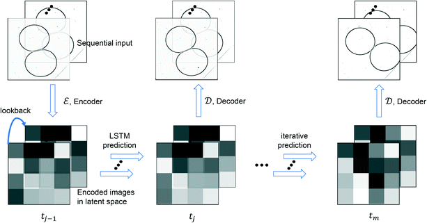
The encoded past image sequence, i.e., hl is referred to the input sequence of the LSTM, and the input and output sequences are of the same length in this study. By iterating the prediction process (eqn (11)), long-term forecasting of a dynamical system can be performed when the initial sequence is provided.28,30
The LSTM surrogate model is implemented in Keras and the layout of the model is shown in Table 2. Two LSTM layers are utilized and three dense layers are added to align the LSTM output's dimension with that of the encoded variable in latent space. The surrogate model is trained by the Adam optimizer with a learning rate of 5 × 10⁻⁵, 1500 epochs. As illustrated in Fig. 3, the surrogate model aims to predict the drop dynamics in the latent space with encoded initial observations.
Table 2 LSTM surrogate model structure
| Layer |
Output shapea |
Activation |
|
N
seq: number of latent variables in encoded image sequence.
|
| Input |
(Nseq, NLS) |
|
| LSTM |
(128) |
ReLU |
| Dropout (10%) |
(128) |
|
| Repeat vector |
(Nseq, 128) |
|
| LSTM |
(Nseq, 128) |
ReLU |
| Dropout (10%) |
(Nseq, 128) |
|
| Time distributed (dense) |
(Nseq, 128) |
|
| Dropout (10%) |
(Nseq, 128) |
|
| Time distributed (dense) |
(Nseq, 64) |
|
| Time distributed (dense) |
(Nseq, NLS) |
|
 |
| | Fig. 3 Schematic of iterative LSTM estimation procedure. | |
Let Npred denotes the number of predictions made by LSTM within a video dataset, and Tpred denotes the set of steps that contains the first frame of these predicted sequences. For simplicity, we shorten the annotation of a predicted latent sequence, [![[x with combining tilde]](https://www.rsc.org/images/entities/b_i_char_0078_0303.gif) tpred,
tpred,![[thin space (1/6-em)]](https://www.rsc.org/images/entities/char_2009.gif) …,
…, ![[x with combining tilde]](https://www.rsc.org/images/entities/b_i_char_0078_0303.gif) tpred+Nseq−1]tpred∈Tpred, to [
tpred+Nseq−1]tpred∈Tpred, to [![[x with combining tilde]](https://www.rsc.org/images/entities/b_i_char_0078_0303.gif) tpred]. An iterative prediction process is illustrated in Fig. 3, and the combined latent surrogate function fsurrogate:
tpred]. An iterative prediction process is illustrated in Fig. 3, and the combined latent surrogate function fsurrogate: ![[Doublestruck R]](https://www.rsc.org/images/entities/i_char_e175.gif) Nseq×NLS →
Nseq×NLS → ![[Doublestruck R]](https://www.rsc.org/images/entities/i_char_e175.gif) Nseq×NLS can be described as
Nseq×NLS can be described as
| | [![[x with combining tilde]](https://www.rsc.org/images/entities/b_i_char_0078_0303.gif) tpred+Nseq] = fsurrogate([xtpred]) tpred+Nseq] = fsurrogate([xtpred]) | (12) |
4.3 Ensemble latent assimilation
In this paper, real-time observations (available every 60 frames = 0.06 s) are used to enhance surrogate model predictions. We develop a novel algorithm scheme that combines the LA and ensemble-type approaches for the specification of error covariance matrices. The latter, which determines the weight of model and observation information, impacts crucially the performance of DA algorithms.54,56
4.3.1 Principle of data assimilation.
Instead of performing DA on the original image, in this study the assimilation is performed in the latent space to avoid the costly reconstruction of performing the assimilation on the full image. For frames in the image dataset, observation frames yt, t ∈ Tobs, from the image set X, and encoder is used to convert the observed image to latent vector ỹt. The assimilation of the encoded image sequence can then be formulated as
| |

| (14) |
where
![[B with combining tilde]](https://www.rsc.org/images/entities/b_i_char_0042_0303.gif) t
t,
![[R with combining tilde]](https://www.rsc.org/images/entities/b_i_char_0052_0303.gif) t
t ∈
![[Doublestruck R]](https://www.rsc.org/images/entities/i_char_e175.gif) NLS×NLS
NLS×NLS represent the error covariance matrices of the background (original prediction)

and observations
ỹtj, respectively, and
K is often referred as the Kalman gain matrix, and
![[H with combining tilde]](https://www.rsc.org/images/entities/b_i_char_0048_0303.gif)
∈
![[Doublestruck R]](https://www.rsc.org/images/entities/i_char_e175.gif) NLS×NLS
NLS×NLS is the observation matrix of

. Since all information of the observed image is known,
![[H with combining tilde]](https://www.rsc.org/images/entities/b_i_char_0048_0303.gif)
is set to the identity matrix
INLS×NLS. Both state and observation prior errors are often assumed to be Gaussian in DA.
25![[B with combining tilde]](https://www.rsc.org/images/entities/b_i_char_0042_0303.gif) t
t,
![[R with combining tilde]](https://www.rsc.org/images/entities/b_i_char_0052_0303.gif) t
t are defined as the covariances of (
![[x with combining tilde]](https://www.rsc.org/images/entities/b_i_char_0078_0303.gif) tb
tb −
![[x with combining tilde]](https://www.rsc.org/images/entities/b_i_char_0078_0303.gif) ttrue
ttrue) and (
![[H with combining tilde]](https://www.rsc.org/images/entities/b_i_char_0048_0303.gif)
![[x with combining tilde]](https://www.rsc.org/images/entities/b_i_char_0078_0303.gif) ttrue
ttrue −
ỹt),
i.e.,
| | (![[x with combining tilde]](https://www.rsc.org/images/entities/b_i_char_0078_0303.gif) tb − tb − ![[x with combining tilde]](https://www.rsc.org/images/entities/b_i_char_0078_0303.gif) ttrue) ∼ ttrue) ∼ ![[scr N, script letter N]](https://www.rsc.org/images/entities/i_char_e52d.gif) (0, (0,![[thin space (1/6-em)]](https://www.rsc.org/images/entities/char_2009.gif) ![[B with combining tilde]](https://www.rsc.org/images/entities/b_i_char_0042_0303.gif) t), ( t), (![[H with combining tilde]](https://www.rsc.org/images/entities/b_i_char_0048_0303.gif) ![[x with combining tilde]](https://www.rsc.org/images/entities/b_i_char_0078_0303.gif) ttrue − ỹt) ∼ ttrue − ỹt) ∼ ![[scr N, script letter N]](https://www.rsc.org/images/entities/i_char_e52d.gif) (0, (0,![[thin space (1/6-em)]](https://www.rsc.org/images/entities/char_2009.gif) ![[R with combining tilde]](https://www.rsc.org/images/entities/b_i_char_0052_0303.gif) t) t) | (15) |
where
0 denotes the vector of zeros with the same dimension of
![[x with combining tilde]](https://www.rsc.org/images/entities/b_i_char_0078_0303.gif) t
t and
![[x with combining tilde]](https://www.rsc.org/images/entities/b_i_char_0078_0303.gif) ttrue
ttrue are the true values of the latent variables at time
t. The latter is out of reach in real data assimilation problems. In LA, equal weights are often assigned to latent predictions and observations,
i.e. assigning
![[B with combining tilde]](https://www.rsc.org/images/entities/b_i_char_0042_0303.gif) t
t and
![[R with combining tilde]](https://www.rsc.org/images/entities/b_i_char_0052_0303.gif) t
t equal to identity matrix
INLS×NLS.
30,53 In this study, performing DA with identity matrices is set as the benchmark, and more sophisticated methods (
e.g. NMC, ensemble) of estimating
![[B with combining tilde]](https://www.rsc.org/images/entities/b_i_char_0042_0303.gif) t
t are employed.
4.3.2 Background error covariance matrix estimation.
To leverage the information embedded in ![[x with combining tilde]](https://www.rsc.org/images/entities/b_i_char_0078_0303.gif) tb and ỹt observations, error covariances specification is a pivotal point in DA. When using ensemble and NMC to compute
tb and ỹt observations, error covariances specification is a pivotal point in DA. When using ensemble and NMC to compute ![[B with combining tilde]](https://www.rsc.org/images/entities/b_i_char_0042_0303.gif) t, the matrix is firstly set to identity at the start of the iterative prediction process, and the value of
t, the matrix is firstly set to identity at the start of the iterative prediction process, and the value of ![[B with combining tilde]](https://www.rsc.org/images/entities/b_i_char_0042_0303.gif) t is updated in the evolution of the latent variables. The correction interval is selected to be 60 frames in this study, and the background error covariance matrix is updated every 60 frames.
4.3.2.1 NMC method.
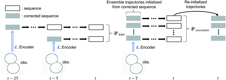
The idea of the NMC approach is to estimate the background error covariance matrix from trajectories that starts from a different initial encoded image sequence. The NMC approach assumes the background errors can be approximated by averaged prediction differences at the same time step, such that
t is updated in the evolution of the latent variables. The correction interval is selected to be 60 frames in this study, and the background error covariance matrix is updated every 60 frames.
4.3.2.1 NMC method.
The idea of the NMC approach is to estimate the background error covariance matrix from trajectories that starts from a different initial encoded image sequence. The NMC approach assumes the background errors can be approximated by averaged prediction differences at the same time step, such that| |  | (16) |
where T represents an arbitrary time interval, and  ,
,  denote two latent variables in trajectories' predictions at time step t with the starting points at t − T and t − 2T, respectively. The derivation of the two latent variables can be formulated as
| | 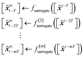 | (17) |
The sequence starting at t − 2T will not be corrected at t − T, and the two trajectories will have different estimations at time step t as shown in Fig. 4. For m trajectories starting from m different starting points, the mean of latent variables in trajectories ![[x with combining tilde]](https://www.rsc.org/images/entities/b_i_char_0078_0303.gif) ′t is defined as:
′t is defined as:| |  | (18) |
The updated background error covariance matrix for each assimilation step can be estimated from| |  | (19) |
 |
| | Fig. 4 Derivation of ![[B with combining tilde]](https://www.rsc.org/images/entities/b_i_char_0042_0303.gif) tNMC and tNMC and ![[B with combining tilde]](https://www.rsc.org/images/entities/b_i_char_0042_0303.gif) tensemble. tensemble. | |
| |  | (20) |
where  ,
,  denote two different disturbed latent variables in trajectories. More precisely, Gaussian noises are added to the background states in the first sequence. For each element in the latent space
 ![[x with combining tilde]](https://www.rsc.org/images/entities/b_i_char_0078_0303.gif) q, the unbiased Gaussian noises are scaled based on the empirical variance against time, i.e.,
q, the unbiased Gaussian noises are scaled based on the empirical variance against time, i.e.,| |  | (21) |
where ![[scr N, script letter N]](https://www.rsc.org/images/entities/i_char_e52d.gif) denotes the normal distribution. The noise coefficient is fixed as σx = 800 in this study after a parameter tuning. Similar to eqn (18), the mean of an ensemble of m disturbed latent trajectories,
denotes the normal distribution. The noise coefficient is fixed as σx = 800 in this study after a parameter tuning. Similar to eqn (18), the mean of an ensemble of m disturbed latent trajectories, ![[x with combining macron]](https://www.rsc.org/images/entities/b_i_char_0078_0304.gif) ′t, is defined as:
′t, is defined as:| |  | (22) |
The updated background error covariance matrix can be estimated from
| |  | (23) |
The trajectories in the ensemble are re-initialized after each correction, the corrected sequence is copied to each trajectory and disturbances are introduced following
eqn (21).
For both NMC and ensemble methods, the estimated ![[B with combining tilde]](https://www.rsc.org/images/entities/b_i_char_0042_0303.gif) t is further processed by the following Gaspari–Cohn covariance localized function69 to mitigate the appearance of spurious error correlations,25
t is further processed by the following Gaspari–Cohn covariance localized function69 to mitigate the appearance of spurious error correlations,25
with
| | 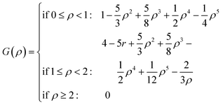 | (24) |
where
i,
j denote the position of elements
![[B with combining tilde]](https://www.rsc.org/images/entities/b_i_char_0042_0303.gif) ti,j
ti,j,
ρ is the distance,
L is the correlation length, and
L is fixed as 2 in this study.
4.3.3 Correction frequency determination.
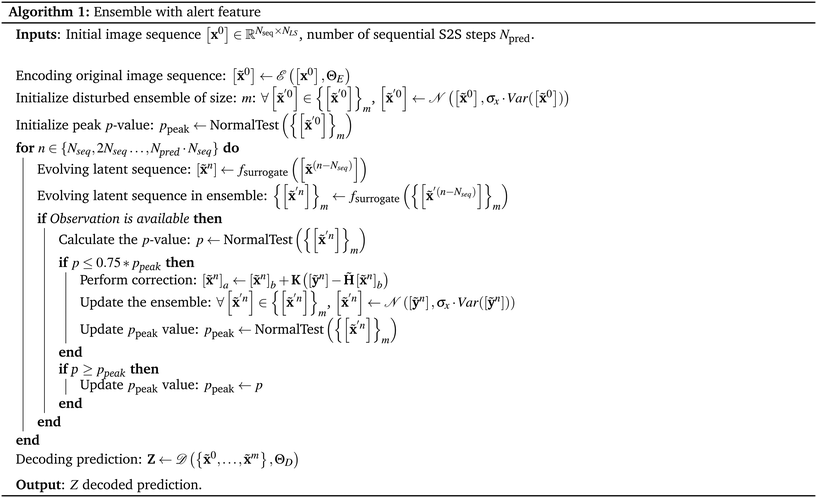
To determine the necessity of correction, the alert feature is implemented in the normally disturbed ensemble method, via monitoring the Gaussianity of the trajectories. When applying Kalman-type DA approaches, the Gaussianity of prior errors is important since approximating non-Gaussian error distributions as Gaussian can lead to erroneous assimilation results.70 To track the Gaussianity of the ensemble, skewness and Kurtosis tests are firstly performed71,72 to measure to what extent the skewness and the outliers of samples in the ensemble differs from the normal distribution. The returned squares of standard scores are summed together, and the Pearson's chi-squared test (χ2, the goodness of fit)73 is performed. The null hypothesis of the test is that the sample follows a normal distribution, and the degree of Gaussianity is quantified by the p-value. Typically, the p-value positively correlates to the confidence of accepting the null hypothesis. Alert is raised once the p-value of trajectories drops below 0.75 of the previous peak p-value, and trajectories will be corrected with the linear interpolated latent sequence. The approach is outlined in Algorithm 1. To the best of our knowledge, no previous implementations which combine machine learning-based reduced-order surrogate models and ensemble-type DA are available in the literature.
To estimate the occurrence of coalescence at the end of S2S prediction, the LA will only be performed on the pre-coalescence stage, and the limit on the number of frames between LA and coalescence/drifting apart image is set to 10. To perform LA, the missing latent space vectors between observations are filled by linear interpolating the latent space elements of two consecutive observations. The element-wise linear interpolation between observations ỹtobs1 and ỹtobs2 is performed as
| |  | (25) |
In this study the observation matrix ![[R with combining tilde]](https://www.rsc.org/images/entities/b_i_char_0052_0303.gif) t is assumed as time-independent (i.e.,
t is assumed as time-independent (i.e., ![[R with combining tilde]](https://www.rsc.org/images/entities/b_i_char_0052_0303.gif) t ≡
t ≡ ![[R with combining tilde]](https://www.rsc.org/images/entities/b_i_char_0052_0303.gif) ), which is a common practice in DA38,36 and LA.30
), which is a common practice in DA38,36 and LA.30![[R with combining tilde]](https://www.rsc.org/images/entities/b_i_char_0052_0303.gif) is computed by calculating the differences between linear interpolated latent observation and the encoded original image in the training set (where
is computed by calculating the differences between linear interpolated latent observation and the encoded original image in the training set (where ![[x with combining tilde]](https://www.rsc.org/images/entities/b_i_char_0078_0303.gif) ttrue is available),
ttrue is available),
Once determined,
![[R with combining tilde]](https://www.rsc.org/images/entities/b_i_char_0052_0303.gif)
is fixed throughout the correction process. The schematic of applying the NMC and the ensemble methods on drop coalescence is shown in
Fig. 4.
5 Results and analysis
In the following section, the performance of reduced-order methods and surrogate models are evaluated by the MSE and L2 norm per element (pixels/latent dimension). The CAE is trained on 8 RTX6000 GPUs using the single-host, multi-device synchronous training strategy implemented in Keras. The LSTM-based surrogate model and LA are trained and computed on a laptop, with an RTX3080 laptop and an Intel 11800H processor.
5.1 Reduced-order methods
The two reduced-order methods (i.e., POD and CAE) are evaluated on the hyperparameter tuning dataset, which consists of 363 frames. Using the training parameters and the evaluating procedure outlined in sec. 4.1.2, the results of different configuration of the CAE is shown in Table 3. The number of layers in the table denotes the depth of the encoder, and configuration 5 has the best overall performance, followed by configuration 1. Considering the time delay caused by encoding observations when performing DA, configuration 1 is selected to minimise the observation error and to reduce the computational cost.
Table 3 CAE configuration grid search
| Label |
Layers |
Filters' size |
Filters |
Max pooling |
MSE |
L
2 norm per pixel |
| 1 |
3 |
162–82–42 |
8–16–32 |
82–82–42 |
5.12 × 10⁻³ |
6.97 × 10⁻⁵ |
| 2 |
3 |
82–82–82 |
8–16–32 |
82–82–42 |
6.78 × 10⁻³ |
8.04 × 10⁻⁵ |
| 3 |
3 |
162–82–42 |
16–16–16 |
82–82–42 |
6.74 × 10⁻³ |
7.99 × 10⁻⁵ |
| 4 |
3 |
82–82–82 |
16–16–16 |
82–82–42 |
6.46 × 10⁻³ |
7.84 × 10⁻⁵ |
| 5 |
4 |
162–82–82–42 |
8–16–16–32 |
42–42–42–42 |
3.87 × 10
−3
|
6.05 × 10
−5
|
| 6 |
4 |
82–82–82–82 |
8–16–16–32 |
42–42–42–42 |
4.76 × 10⁻³ |
7.00 × 10⁻⁵ |
| 7 |
4 |
162–82–82–42 |
16–16–16–16 |
42–42–42–42 |
5.39 × 10⁻³ |
7.10 × 10⁻⁵ |
| 8 |
4 |
82–82–82–82 |
16–16–16–16 |
42–42–42–42 |
4.06 × 10⁻³ |
6.20 × 10⁻⁵ |
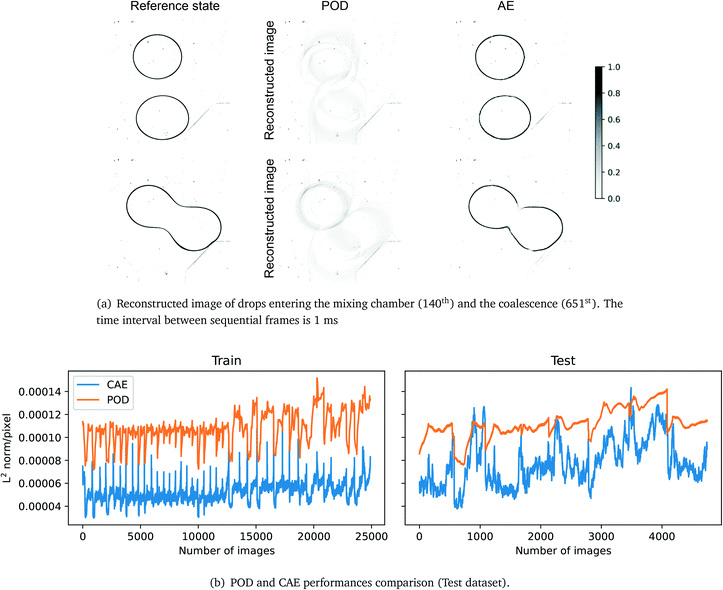
Fig. 5 shows the results of POD and CAE under 16 modes and latent variables, respectively. The diagram demonstrates that POD fails to reconstruct the input image with 16 modes while the CAE can reconstruct sharp images and the average deviation is in a few pixels. Fig. 5b compares the performances of POD and CAE, and the MSE shows the CAE outperforms POD by 77% and 49% on the training and testing datasets, respectively. The spikes shown in Fig. 5b in CAE's training dataset are caused by the further partitioning of the training dataset, i.e. 7/15 of images in the training dataset are equivalent to validation images. The reconstruction quality of the CAE drops as it approaches the coalescence stage, it could be caused by the imbalance of the pre-coalescence stage and (post-)coalescence stage images. The two related factors are the selection of CAE's training dataset, and the lack of post-coalescence images, as the camera stops recording once the coalescence happens, thus, few coalesced images are included in the CAE's training dataset. The 3-layer CAE is selected for the encoding and decoding process as it outperforms the POD.
 |
| | Fig. 5 Figurative and numerical comparison of the two reduced-order methods. POD: MSE: 1.23 × 10⁻² (train), 1.33 × 10⁻² (test); L2 norm per pixel: 1.08 × 10⁻⁴ (train), 1.12 × 10⁻⁴ (test). CAE: MSE: 2.86 × 10⁻³ (train), 6.74 × 10⁻³ (test); L2 norm per pixel: 5.16 × 10⁻⁵ (train), 7.77 × 10⁻⁵ (test). | |
5.2 LSTM performance
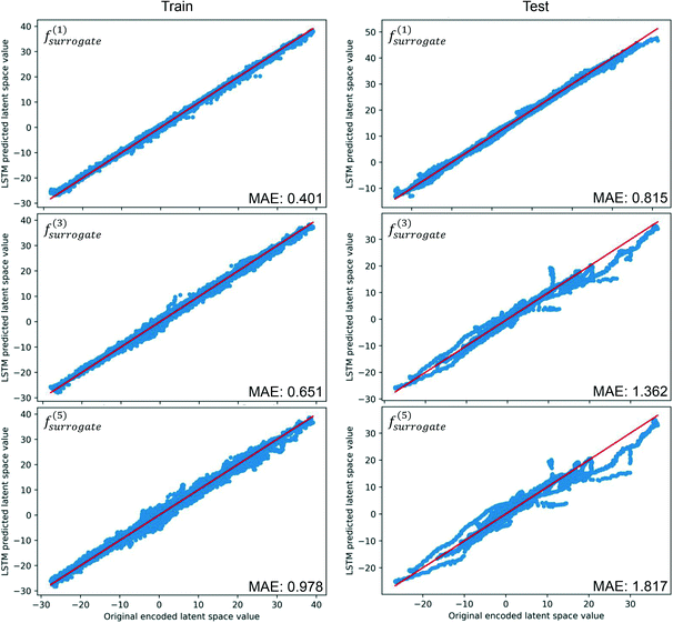
The trained CAE is used to encode all the images in the training and test datasets. To evaluate the performance of the trained LSTM, the MAE is computed by comparing the latent estimation to the corresponding encoding image, and the estimations of the widest span latent variable are illustrated in Fig. 6. Following the notation in eqn (17), the symbol m in f(m)surrogate denotes the number of iterative estimations performed. The predictions of the data-driven surrogate model on the first following sequence can align well with the original encoded images, and the MAE of the following sequences on the test dataset is about twice the error of the training dataset. However, the deviation of estimated values develops quickly on the test dataset, indicating that correction is critical to the accuracy of the S2S predictions. The deviations accumulate on the two datasets, and they are likely caused by the randomness of the dynamics, where two images of similar drops' positions can have different movements.
 |
| | Fig. 6 Results of iterative S2S estimations on the widest span latent variable, MAE is computed by comparing the differences between the estimated and the true latent variables. | |
5.3 Latent assimilation performances
The numerical comparison of different DA methods on the latent variables in the test dataset is outlined in Table 4, and errors are computed by comparing decoded latent variables to reference images. It should be noted that only the initial sequence and a series of observations before the coalescence/drifting apart are provided to the surrogate model. The AE-Identity% indicates the improvement (in terms of L2 error) of each method compared to the standard LA approach using identity covariance matrices. As observed in Table 4, the ensemble (5) exhibits the best score of AE-Identity% with +9%, followed by the NMC (5) with +5.8%. Furthermore, the ensemble (25) with the alert feature has a similar numerical performance to the identity approach, with a lower correction frequency. The CAE reconstructed image and the decoded observation have the same magnitude of errors, and it shows that the variation in latent variables' value can be well approximated by the linear interpolation. The computation cost of the surrogate model can be reflected by the computation time, which includes the time taken to evolve trajectories. The trajectories in the NMC and ensemble methods are computed in serial, and the computation time of the two methods can be reduced once they are parallelized. Generally, there exists a trade-off between the accuracy of estimations and the computation time, due to the positive correlation between the number of tracked trajectories and the computed background covariance matrix. The last image in the test datasets and the predicted trajectory is used to evaluate if the surrogate model successfully predicts the coalescence. The original image transferred by the encoding-decoding process is referred to the CAE reconstructed image, and it is treated as the “ground truth” for the surrogate model because it indicates the best result that the S2S surrogate model can achieve.
Table 4 Errors of surrogate model on test dataset
|
N
seq
|
Reconstruction |
Correction interval.(frames) |
MSE |
L
2 error per pixel |
MSEa (AE-Id%) |
Computation time (s) |
|
|
AE reconstruction |
|
6.74 × 10⁻³ |
7.77 × 10⁻⁵ |
100% |
|
|
|
Linear interpolated observation |
60 |
7.46 × 10⁻³ |
8.22 × 10⁻⁵ |
94.1% |
|
| Methods |
|
(MSEidentity − MSE)/(MSEidentity − MSEAE).
Numbers in brackets denote the number of trajectories.
Average of images within correction interval.
|
| 5 |
LSTM, no correction |
|
2.54 × 10⁻² |
1.54 × 10⁻⁴ |
−53.5% |
3.3
|
| 5 |
Identity |
60 |
1.89 × 10⁻² |
1.32 × 10⁻⁴ |
0% |
3.4 |
| 5 |
NMC (5)b |
60 |
1.82 × 10⁻² |
1.29 × 10⁻⁴ |
5.8% |
9.0 |
| 5 |
Ensemble (5) |
60 |
1.78 × 10
−2
|
1.27 × 10
−4
|
9.0%
|
18.6 |
| 5 |
Ensemble (25), with alert |
85
|
1.92 × 10⁻² |
1.32 × 10⁻⁴ |
2.5% |
83.1 |
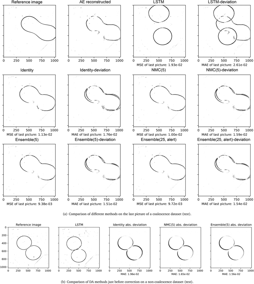
A set of the final images of different DA methods are presented in Fig. 8(a), their MSE/MAE are calculated from comparing decoded estimations and decoded images. Among the eight test videos, the surrogate model without correction (LSTM) fails to predict any coalescence, and the predicted drops have large deviations in shape. The identity, NMC (5) and ensemble (5) methods have smaller errors, and the predicted shapes of the drops are similar. The three methods estimated five out of eight outcomes correctly including one of the coalesced drops are shown in Fig. 8(a). Without the alert feature, the ensemble (25) can estimate six out of eight outcomes correctly with a correction interval of 60 frames. On average, the ensemble (25) with the alert feature can estimate five outcomes correctly with an average correction interval of 85 frames, and the average number of corrections performed on each test dataset is 6.5. By comparing the MSE of decoded latent variables of the LSTM and the ensemble (25) with alerts, the similarity in errors and differences in shape demonstrate the alert feature works effectively. The alert method achieves comparable performance in predicting the outcomes of the two drops, and its MSE and L2 error are close to the identity matrix approach with a shorter correction interval. Fig. 8(b) compares the absolute deviation of the three LA techniques at the time step where a correction is about to perform, i.e., 60 frames after the previous correction. NMC and ensemble methods generally perform better than the identity matrix approach, when the deviations from the reference state are not too large, and it implies the ensemble and the NMC can estimate the background covariance matrix robustly.
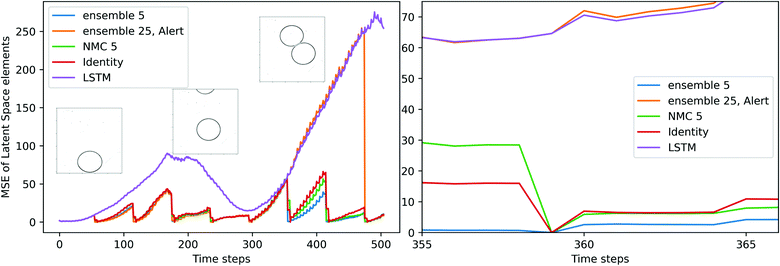
Fig. 7 illustrates the evolving of latent variables' MSE in the previously shown coalesced test dataset, and two corrections are skipped near the end of the sequence. The MSE of S2S LSTM shows a trend of fluctuation. The reduction of MSE occurs when the upper drop enters the chamber and the two drops approach each other, then the error develops quickly when the two drops are about to make contact, as the interactions between drops increase at this stage. The alert is raised at 480th image (i.e., 0.48 s) and the S2S LSTM successfully estimates the coalescence at the end of the test dataset. The alert feature also serves as an indication of process uncertainty. In the case of Fig. 7, the tip of the upper drop starts to enter the chamber around the 200th image. Correction is constantly requested at this stage because the CAE-LSTM has not yet fully captured the shape of the drops, and it is reflected by the divergence of disturbed trajectories within the ensemble.
 |
| | Fig. 7 Comparison of the MSE of the latent vector on the coalesced test dataset and its enlarged version. The three snapshots extracted from frames 1, 200, and 400 of the original video. Each time step is equivalent to ×10−3 seconds. | |
 |
| | Fig. 8 Figurative and numerical comparison of different methods on test datasets. | |
6 Conclusion and future work
In this study, an image-based data-driven model is built to predict the dynamics of drop interactions in a microfludic device based on experimental data. Ordered sequences are constructed from encoded videos and a S2S LSTM is trained for predictions in the reduced-order latent space. Observation (images extracted from unseen experiment data) is introduced to monitor the real-time prediction of drop dynamics thanks to LA algorithms. We developed a novel algorithm scheme that combines the LSTM-based surrogate modelling and Ensemble-type LA algorithms in reduced-order latent spaces. As a first attempt at an efficient ROM- and DL-based surrogate model for microfluidics drop dynamics, the results obtained in this work highlight the potential of data-driven models for predicting the coalescence probability and guiding the choice of experiment parameters.
The performances of LSTM with different LA techniques show the NMC and ensemble methods outperform the identity approach, as both methods show positive improvements on the MSE and the L2 error of the adjusted predictions. It indicates that having a good estimation of the background covariance matrix is beneficial to the overall assimilated result. Although the sample size is relatively small, the data-driven surrogate model estimates five out of eight outcomes correctly for a correction interval of 60 frames (a correction frequency of two seconds). A robust correction determination method is proposed and implemented based on the ensemble method, and the implemented alert feature can predict at most six outcomes correctly.
In terms of future work, the quality of datasets can be improved by recording more frames after the coalescence/drifting apart to reduce the imbalance between pre-coalescence and coalescence's images. Various RNN structures can be tested, for instance, gated recurrent unit (GRU)74 and attention-based RNN,75 to further increase the performance of the surrogate model. To improve the generalizability of the proposed approach, more combinations of phase velocities can be included in the LSTM's training set to investigate the correlation between the variety of datasets and model performance, as the current dataset only covers two combinations of velocities. The datasets could be extended further to various device geometries, for example, various sizes of coalescence chamber. Such extension of training datasets will enable optimisation of geometry and flow rates resulting in close to 100% coalescence rate. Securing the high coalescence rate is crucial for microfluidic reactions and screening. Examples are drug screening where some acting ingredients can be added dropwise and close to 100% coalescence rate will guarantee similar environment in each screening unit or synthesis of hydrogels where non-coalesced drops can lead to device clogging. In addition, a CFD simulator of drop dynamics is under development and future ML approaches can learn from these high-fidelity simulations to enhance the performance of the current approach. Furthermore, using the current surrogate model these CFD data can be used as observations in DA to prevent non-realistic predictions. When more experimental/CFD data with different initial conditions are available, further work can be investigated to develop an operational algorithm to predict the probability of coalescence via initial observations. In addition, the LA methods proposed in this study are applicable for studying dynamics other than coalescence, and the LA combined LSTM-based surrogate model shows promising results on estimating complex dynamics.
Acronyms
| NN | Neural networks |
| ML | Machine learning |
| LA | Latent assimilation |
| DA | Data assimilation |
| AE | Autoencoder |
| CAE | Convolutional autoencoder |
| RNN | Recurrent neural network |
| CNN | Convolutional neural network |
| LSTM | Long short-term memory |
| POD | Proper orthogonal decomposition |
| SVD | Singular value decomposition |
| ROM | Reduced-order modelling |
| CFD | Computational fluid mechanics |
| 1D | One-dimensional |
| MSE | Mean square error |
| MAE | Mean absolute error |
| S2S | Sequence-to-sequence |
| DL | Deep learning |
Conflicts of interest
There are no conflicts to declare.
Acknowledgements
This research is funded by the EP/T000414/1 PREdictive Modelling with QuantIfication of UncERtainty for MultiphasE Systems (PREMIERE). This work is partially supported by the Leverhulme Centre for Wildfires, Environment and Society through the Leverhulme Trust, grant number RC-2018-023. The authors are grateful to two anonymous reviewers for the useful suggestions on the manuscript.
Notes and references
- G. M. Whitesides, Nature, 2006, 442, 368–373 CrossRef CAS PubMed.
- M. Joanicot and A. Ajdari, Science, 2005, 309, 887–888 CrossRef CAS PubMed.
- A. S. Utada, E. Lorenceau, D. R. Link, P. D. Kaplan, H. A. Stone and D. A. Weitz, Science, 2005, 308, 537–541 CrossRef CAS PubMed.
- T. Krebs, K. Schroen and R. Boom, Lab Chip, 2012, 12, 1060–1070 RSC.
- K. Schroen, C. Berton-Carabin, D. Renard, M. Marquis, A. Boire, R. Cochereau, C. Amine and S. Marze, Micromachines, 2021, 12, 863 CrossRef PubMed.
- H. Shi, K. Nie, B. Dong, M. Long, H. Xu and Z. Liu, Chem. Eng. J., 2019, 361, 635–650 CrossRef CAS.
- A. Stucki, J. Vallapurackal, T. R. Ward and P. S. Dittrich, Angew. Chem., Int. Ed., 2021, 60, 24368–24387 CrossRef CAS PubMed.
- S. Sarkar, N. Cohen, P. Sabhachandani and T. Konry, Lab Chip, 2015, 15, 4441–4450 RSC.
- S. Sarkar, P. Sabhachandani, D. Stroopinsky, K. Palmer, N. Cohen, J. Rosenblatt, D. Avigan and T. Konry, Biomicrofluidics, 2016, 10, 054115 CrossRef CAS PubMed.
- M. Solsona, J. C. Vollenbroek, C. B. M. Tregouet, A.-E. Nieuwelink, W. Olthuis, A. van den Berg, B. M. Weckhuysen and M. Odijk, Lab Chip, 2019, 19, 3575–3601 RSC.
- V. P. Galván-Chacón, L. Costa, D. Barata and P. Habibovic, Acta Biomater., 2021, 128, 486–501 CrossRef PubMed.
- A. Moreira, J. Carneiro, J. B. L. M. Campos and J. M. Miranda, Microfluid. Nanofluid., 2021, 25, 10 CrossRef CAS.
- S. Kubendhiran, Z. Bao, K. Dave and R.-S. Liu, ACS Appl. Nano Mater., 2019, 2, 1773–1790 CrossRef CAS.
- K. Nathanael, P. Pico, N. M. Kovalchuk, A. D. Lavino, M. J. Simmons and O. K. Matar, Chem. Eng. J., 2022, 135178 CrossRef CAS.
- C. Hirt and B. Nichols, J. Comput. Phys., 1981, 39, 201–225 CrossRef.
- G. Tryggvason, B. Bunner, A. Esmaeeli, D. Juric, N. Al-Rawahi, W. Tauber, J. Han, S. Nas and Y.-J. Jan, J. Comput. Phys., 2001, 169, 708–759 CrossRef CAS.
- S. Osher and J. A. Sethian, J. Comput. Phys., 1988, 79, 12–49 CrossRef.
- T. Glatzel, C. Litterst, C. Cupelli, T. Lindemann, C. Moosmann, R. Niekrawietz, W. Streule, R. Zengerle and P. Koltay, Comput. Fluids, 2008, 37, 218–235 CrossRef.
- K. Sambath, V. Garg, S. S. Thete, H. J. Subramani and O. A. Basaran, J. Fluid Mech., 2019, 876, 449–480 CrossRef CAS.
- A. R. Guzman, H. S. Kim, P. de Figueiredo and A. Han, Biomed. Microdevices, 2015, 17, 35 CrossRef PubMed.
- A. Shenoy, C. V. Rao and C. M. Schroeder, Proc. Natl. Acad. Sci. U. S. A., 2016, 113, 3976–3981 CrossRef CAS PubMed.
- S. Narayan, I. Makhnenko, D. B. Moravec, B. G. Hauser, A. J. Dallas and C. S. Dutcher, Langmuir, 2020, 36, 9827–9842 CrossRef CAS PubMed.
- G. I. Taylor, Proc. R. Soc. London, Ser. A, 1934, 146, 501–523 CAS.
- H. Yi, T. Fu, C. Zhu and Y. Ma, Chem. Eng. J., 2022, 430, 133087 CrossRef CAS.
- A. Carrassi, M. Bocquet, L. Bertino and G. Evensen, Wiley Interdiscip. Rev. Clim. Change, 2018, 9, e535 Search PubMed.
-
W. H. Schilders, H. A. Van der Vorst and J. Rommes, Model order reduction: theory, research aspects and applications, Springer, 2008, vol. 13 Search PubMed.
- T. Nakamura, K. Fukami, K. Hasegawa, Y. Nabae and K. Fukagata, Phys. Fluids, 2021, 33, 025116 CrossRef CAS.
- K. Fukami, K. Fukagata and K. Taira, Theor. Comput. Fluid Dyn., 2020, 34, 497–519 CrossRef.
- C. Q. Casas, R. Arcucci, P. Wu, C. Pain and Y.-K. Guo, Phys. D, 2020, 412, 132615 CrossRef.
-
M. Amendola, R. Arcucci, L. Mottet, C. Q. Casas, S. Fan, C. Pain, P. Linden and Y.-K. Guo, Data Assimilation in the Latent Space of a Neural Network, 2020 Search PubMed.
- S. Cheng, I. C. Prentice, Y. Huang, Y. Jin, Y.-K. Guo and R. Arcucci, J. Comput. Phys., 2022, 111302 CrossRef.
-
J. Lumley, Atmospheric turbulence and radio wave propagation, 1967 Search PubMed.
- B. Moore, IEEE Trans. Autom. Control, 1981, 26, 17–32 CrossRef.
- C. W. Rowley, I. Mezic, S. Bagheri, P. Schlatter and D. S. Henningson, J. Fluid Mech., 2009, 641, 115–127 CrossRef.
- P. J. Schmid, J. Fluid Mech., 2010, 656, 5–28 CrossRef CAS.
- R. Arcucci, L. Mottet, C. Pain and Y.-K. Guo, J. Comput. Phys., 2019, 379, 51–69 CrossRef.
- C. W. Rowley, Int. J. Bifurcation Chaos Appl. Sci. Eng., 2005, 15, 997–1013 CrossRef.
- S. Cheng, D. Lucor and J.-P. Argaud, J. Comput. Sci., 2021, 101405 CrossRef.
- R. Maulik, K. Fukami, N. Ramachandra, K. Fukagata and K. Taira, Phys. Rev. Fluids, 2020, 5, 104401 CrossRef.
- Y. Fan, G. Wen, D. Li, S. Qiu, M. D. Levine and F. Xiao, Comput. Vis. Image Underst., 2020, 195, 102920 CrossRef.
-
K. Simonyan and A. Zisserman, Two-Stream Convolutional Networks for Action Recognition in Videos, 2014 Search PubMed.
- T. R. Phillips, C. E. Heaney, P. N. Smith and C. C. Pain, Int. J. Numer. Methods Eng., 2021, 122, 3780–3811 CrossRef.
-
Y. Zhou, C. Wu, Z. Li, C. Cao, Y. Ye, J. Saragih, H. Li and Y. Sheikh, 2020, arXiv preprint arXiv:2006.04325.
- G. E. Hinton and R. R. Salakhutdinov, Science, 2006, 313, 504–507 CrossRef CAS PubMed.
-
L. Fulton, V. Modi, D. Duvenaud, D. I. W. Levin and A. Jacobson, Computer Graphics Forum, 2019 Search PubMed.
- C. Liu, R. Fu, D. Xiao, R. Stefanescu, P. Sharma, C. Zhu, S. Sun and C. Wang, Eng. Anal. Bound. Elem., 2022, 139, 46–55 CrossRef.
- D. E. Rumelhart, G. E. Hinton and R. J. Williams, Nature, 1986, 323, 533–536 CrossRef.
- Y. Bengio, P. Simard and P. Frasconi, IEEE Trans. Neural Netw., 1994, 5, 157–166 CAS.
- K. Greff, R. K. Srivastava, J. Koutnik, B. R. Steunebrink and J. Schmidhuber, IEEE Trans. Neural Netw. Learn. Syst., 2017, 28, 2222–2232 Search PubMed.
- S. Hochreiter and J. Schmidhuber, Neural Comput., 1997, 9, 1735–1780 CrossRef CAS PubMed.
-
J. N. Kani and A. H. Elsheikh, DR-RNN: A deep residual recurrent neural network for model reduction, 2017 Search PubMed.
- Z. Wang, D. Xiao, F. Fang, R. Govindan, C. C. Pain and Y. Guo, Int. J. Numer. Methods Fluids, 2018, 86, 255–268 CrossRef CAS.
-
M. Peyron, A. Fillion, S. Gürol, V. Marchais, S. Gratton, P. Boudier and G. Goret, 2021, arXiv preprint arXiv:2104.00430.
- S. Cheng, J.-P. Argaud, B. Iooss, D. Lucor and A. Ponçot, Stochastic Environ. Res. Risk Assess., 2019, 33, 2033–2051 CrossRef.
-
M. Fisher, Seminar on Recent developments in data assimilation for atmosphere and ocean (Shinfield Park, Reading, 8–12 September), 2003 Search PubMed.
- G. Desroziers, L. Berre, B. Chapnik and P. Poli, Q. J. R. Meteorol. Soc., 2005, 131, 3385–3396 CrossRef.
- S. Cheng and M. Qiu, Neural. Comput. Appl., 2021, 1–19 Search PubMed.
- J. R. Eyre and F. I. Hilton, Q. J. R. Meteorol. Soc., 2013, 139, 524–533 CrossRef.
- E. Lin, Y. Yang, X. Qiu, Q. Xie, R. Gan, B. Zhang and X. Liu, Atmos. Res., 2021, 257, 105590 CrossRef.
- H. He, L. Lei, J. S. Whitaker and Z.-M. Tan, J. Adv. Model. Earth Syst., 2020, 12, e2020MS002187 Search PubMed.
- D. F. Parrish and J. C. Derber, Mon. Weather Rev., 1992, 120, 1747–1763 CrossRef.
- G. Evensen, J. Geophys. Res.: Oceans, 1994, 99, 10143–10162 CrossRef.
- M. Bocquet and A. Carrassi, Tellus B, 2017, 69, 1304504 CrossRef.
- P. Kim, K. W. Kwon, M. C. Park, S. H. Lee, S. M. Kim and K. Y. Suh, BioChip J., 2008, 2, 1–11 Search PubMed.
- Y. Wang, H. Yao and S. Zhao, Neurocomputing, 2016, 184, 232–242 CrossRef.
-
S. E. Otto and C. W. Rowley, Linearly-Recurrent Autoencoder Networks for Learning Dynamics, 2019 Search PubMed.
-
F. J. Gonzalez and M. Balajewicz, Deep convolutional recurrent autoencoders for learning low-dimensional feature dynamics of fluid systems, 2018 Search PubMed.
-
D. P. Kingma and J. Ba, Adam: A Method for Stochastic Optimization, 2017 Search PubMed.
- G. Gaspari and S. E. Cohn, Q. J. R. Meteorol. Soc., 1999, 125, 723–757 CrossRef.
- A. Fowler and P. Jan Van Leeuwen, Tellus B, 2013, 65, 20035 CrossRef.
- R. D'Agostino and E. S. Pearson, Biometrika, 1973, 60, 613–622 Search PubMed.
- R. B. D'Agostino, Biometrika, 1971, 58, 341–348 CrossRef.
- K. Pearson, Philos. Mag., 1900, 50, 157–175 Search PubMed.
-
J. Chung, C. Gulcehre, K. Cho and Y. Bengio, 2014, arXiv preprint arXiv:1412.3555.
- M. E. Basiri, S. Nemati, M. Abdar, E. Cambria and U. R. Acharya, Future Gener. Comput. Syst., 2021, 115, 279–294 CrossRef.
|
| This journal is © The Royal Society of Chemistry 2022 |
 Open Access Article
 *b,
Nina
Kovalchuk
 c,
Mark
Simmons
c,
Omar K.
Matar
a,
Yi-Ke
Guo
b and
Rossella
Arcucci
*bd
c,
Mark
Simmons
c,
Omar K.
Matar
a,
Yi-Ke
Guo
b and
Rossella
Arcucci
*bd
![[thin space (1/6-em)]](https://www.rsc.org/images/entities/char_2009.gif) :
:![[thin space (1/6-em)]](https://www.rsc.org/images/entities/char_2009.gif) 5. Drops of dispersed phase were formed in two symmetrical flow-focusing cross-junctions 4 and were then transferred by continuous phase to chamber 5 where they meet and then either coalesce or not, and exit the chamber through the symmetrical output channel 3. The parameters affecting coalescence are the total flow rate, the viscosities of the continuous and dispersed phase, the interfacial tension, the presence of surfactant in the continuous or dispersed phase and surfactant properties. The drop size depends on all other parameters and time-lag between the drops arrival to the chamber. In this study, only flow rates and drop lag time were varied whereas all other parameters were kept constant. Drop size was varied slightly (within 5%) due to changes in the flow rate.
5. Drops of dispersed phase were formed in two symmetrical flow-focusing cross-junctions 4 and were then transferred by continuous phase to chamber 5 where they meet and then either coalesce or not, and exit the chamber through the symmetrical output channel 3. The parameters affecting coalescence are the total flow rate, the viscosities of the continuous and dispersed phase, the interfacial tension, the presence of surfactant in the continuous or dispersed phase and surfactant properties. The drop size depends on all other parameters and time-lag between the drops arrival to the chamber. In this study, only flow rates and drop lag time were varied whereas all other parameters were kept constant. Drop size was varied slightly (within 5%) due to changes in the flow rate.![[Doublestruck R]](https://www.rsc.org/images/entities/i_char_e175.gif) 1024×1024. The video (image dataset) can then be denoted as a matrix X = [xt1,
1024×1024. The video (image dataset) can then be denoted as a matrix X = [xt1,![[thin space (1/6-em)]](https://www.rsc.org/images/entities/char_2009.gif) ⋯xtm] ∈
⋯xtm] ∈ ![[Doublestruck R]](https://www.rsc.org/images/entities/i_char_e175.gif) 1024×1024×m. For applying the vectorwise POD algorithm, state vectors xt will be flattened into (1D) vectors in the rest of sec. 4.1.1, where the new dimensions are xtM ∈
1024×1024×m. For applying the vectorwise POD algorithm, state vectors xt will be flattened into (1D) vectors in the rest of sec. 4.1.1, where the new dimensions are xtM ∈ ![[Doublestruck R]](https://www.rsc.org/images/entities/i_char_e175.gif) 10242, X = ∈
10242, X = ∈ ![[Doublestruck R]](https://www.rsc.org/images/entities/i_char_e175.gif) 10242×m. The image set matrix can be projected to a low-dimensional latent space via (SVD):
10242×m. The image set matrix can be projected to a low-dimensional latent space via (SVD):
![[thin space (1/6-em)]](https://www.rsc.org/images/entities/char_2009.gif) u2⋯ur] ∈
u2⋯ur] ∈ ![[Doublestruck R]](https://www.rsc.org/images/entities/i_char_e175.gif) 10242×r, Σ ∈
10242×r, Σ ∈ ![[Doublestruck R]](https://www.rsc.org/images/entities/i_char_e175.gif) r×r is a diagonal matrix with positive entries, σ1, σ2, ⋯, σr, and V = [v1v2⋯vr] ∈
r×r is a diagonal matrix with positive entries, σ1, σ2, ⋯, σr, and V = [v1v2⋯vr] ∈ ![[Doublestruck R]](https://www.rsc.org/images/entities/i_char_e175.gif) m×r. The columns of U and V are orthonormal such that
m×r. The columns of U and V are orthonormal such that![[X with combining tilde]](https://www.rsc.org/images/entities/b_i_char_0058_0303.gif) = [
= [![[x with combining tilde]](https://www.rsc.org/images/entities/b_i_char_0078_0303.gif) t1,
t1,![[thin space (1/6-em)]](https://www.rsc.org/images/entities/char_2009.gif) ⋯
⋯![[x with combining tilde]](https://www.rsc.org/images/entities/b_i_char_0078_0303.gif) tm] ∈
tm] ∈ ![[Doublestruck R]](https://www.rsc.org/images/entities/i_char_e175.gif) d×m can be calculated from:
d×m can be calculated from:![[X with combining tilde]](https://www.rsc.org/images/entities/b_i_char_0058_0303.gif) = UTdX, and
= UTdX, and ![[x with combining tilde]](https://www.rsc.org/images/entities/b_i_char_0078_0303.gif) t = UTdxt
t = UTdxt![[X with combining tilde]](https://www.rsc.org/images/entities/b_i_char_0058_0303.gif) , and
, and![[thin space (1/6-em)]](https://www.rsc.org/images/entities/char_2009.gif) zt = UTd
zt = UTd![[x with combining tilde]](https://www.rsc.org/images/entities/b_i_char_0078_0303.gif) t
t
![[x with combining tilde]](https://www.rsc.org/images/entities/b_i_char_0078_0303.gif) t. The fully connected (dense) layers in AE work well with small-scale problems (∼103 degrees of freedom,65,66) but has trouble handling problems characterised by higher degrees of freedom (e.g. 106–109).67 CAE is adopted in this work to exploit the spatial neighbouring correlations.
t. The fully connected (dense) layers in AE work well with small-scale problems (∼103 degrees of freedom,65,66) but has trouble handling problems characterised by higher degrees of freedom (e.g. 106–109).67 CAE is adopted in this work to exploit the spatial neighbouring correlations.
![[Doublestruck R]](https://www.rsc.org/images/entities/i_char_e175.gif) 1024×1024 with filters (kernels) to generate feature maps by trainable weights. For Nk kernel in a convolutional layer with filter KNk ∈
1024×1024 with filters (kernels) to generate feature maps by trainable weights. For Nk kernel in a convolutional layer with filter KNk ∈ ![[Doublestruck R]](https://www.rsc.org/images/entities/i_char_e175.gif) a×b and filter size (a × b), an element located at (i, j) in the corresponding generated feature map (x * KNk) can be expressed as:
a×b and filter size (a × b), an element located at (i, j) in the corresponding generated feature map (x * KNk) can be expressed as:
![[x with combining tilde]](https://www.rsc.org/images/entities/b_i_char_0078_0303.gif) t.
t.
![[x with combining tilde]](https://www.rsc.org/images/entities/b_i_char_0078_0303.gif) t =
t = ![[scr E, script letter E]](https://www.rsc.org/images/entities/i_char_e140.gif) (xt,
(xt,![[thin space (1/6-em)]](https://www.rsc.org/images/entities/char_2009.gif) ΘE), zt =
ΘE), zt = ![[scr D, script letter D]](https://www.rsc.org/images/entities/i_char_e523.gif) (
(![[x with combining tilde]](https://www.rsc.org/images/entities/b_i_char_0078_0303.gif) t,
t,![[thin space (1/6-em)]](https://www.rsc.org/images/entities/char_2009.gif) ΘD)
ΘD)![[scr E, script letter E]](https://www.rsc.org/images/entities/char_e140.gif) :
: ![[Doublestruck R]](https://www.rsc.org/images/entities/i_char_e175.gif) 1024×1024 →
1024×1024 → ![[Doublestruck R]](https://www.rsc.org/images/entities/i_char_e175.gif) NLS,
NLS, ![[scr D, script letter D]](https://www.rsc.org/images/entities/i_char_e523.gif) :
: ![[Doublestruck R]](https://www.rsc.org/images/entities/i_char_e175.gif) NLS →
NLS → ![[Doublestruck R]](https://www.rsc.org/images/entities/i_char_e175.gif) 1024×1024 denote the encoder and the decoder, which are parameterized by ΘE and ΘD, respectively, and NLS denotes the dimension of the latent space.
1024×1024 denote the encoder and the decoder, which are parameterized by ΘE and ΘD, respectively, and NLS denotes the dimension of the latent space.
 and
and  are determined from the binary cross-entropy loss function
![[Doublestruck R]](https://www.rsc.org/images/entities/i_char_e175.gif) 1024×1024 denotes the matrix of ones. In this work, cross-entropy is employed as loss function instead of MSE or MAE because of the data imbalance, that is, the drop interface only represents a small number of pixels in each image. Using MSE or MAE as loss function will lead to predictions of blank images. The values of the reconstructed matrix are normalized between 0 and 1 to bound the predicted values. Using the optimal hyperparameters determined from the parameter tuning dataset, the CAE is implemented in Keras and a detailed structure of the selected hyperparameters of the CAE is shown in Table 1, where ReLU denotes rectified linear unit. The CAE is trained with the gradient-based optimizer, Adam,68 with a learning rate of 5 × 10⁻⁵, 5000 epochs, and the loss is computed using binary cross-entropy due to the imbalance in grey-scale pixels. The hyperparamter tuning concerning the structure of the CAE is latter displayed in section 5. The dimension of the latent space, 16, is selected based on the optimal latent space dimension to image matrix size ratio (5.2 × 10⁻⁵) proposed in ref. 30, and the structure of the coalescence chamber, where only around half of the space in images is occupied by the actual chamber.
1024×1024 denotes the matrix of ones. In this work, cross-entropy is employed as loss function instead of MSE or MAE because of the data imbalance, that is, the drop interface only represents a small number of pixels in each image. Using MSE or MAE as loss function will lead to predictions of blank images. The values of the reconstructed matrix are normalized between 0 and 1 to bound the predicted values. Using the optimal hyperparameters determined from the parameter tuning dataset, the CAE is implemented in Keras and a detailed structure of the selected hyperparameters of the CAE is shown in Table 1, where ReLU denotes rectified linear unit. The CAE is trained with the gradient-based optimizer, Adam,68 with a learning rate of 5 × 10⁻⁵, 5000 epochs, and the loss is computed using binary cross-entropy due to the imbalance in grey-scale pixels. The hyperparamter tuning concerning the structure of the CAE is latter displayed in section 5. The dimension of the latent space, 16, is selected based on the optimal latent space dimension to image matrix size ratio (5.2 × 10⁻⁵) proposed in ref. 30, and the structure of the coalescence chamber, where only around half of the space in images is occupied by the actual chamber.
![[x with combining tilde]](https://www.rsc.org/images/entities/b_i_char_0078_0303.gif) ∈
∈ ![[Doublestruck R]](https://www.rsc.org/images/entities/i_char_e175.gif) NLS, the output vector h ∈
NLS, the output vector h ∈ ![[Doublestruck R]](https://www.rsc.org/images/entities/i_char_e175.gif) NLS of a single layer in feed-forward network can be computed as
NLS of a single layer in feed-forward network can be computed as![[x with combining tilde]](https://www.rsc.org/images/entities/b_i_char_0078_0303.gif) + b)
+ b)![[Doublestruck R]](https://www.rsc.org/images/entities/i_char_e175.gif) Nh×NLS denotes the weight matrix, and b ∈
Nh×NLS denotes the weight matrix, and b ∈ ![[Doublestruck R]](https://www.rsc.org/images/entities/i_char_e175.gif) Nh denotes the bias term, and the Sigmoid is the element-wise activation function. Using hl to denote layer l's output of the low-dimensional representation, a deep neural networks can be reformulated from eqn (9),
Nh denotes the bias term, and the Sigmoid is the element-wise activation function. Using hl to denote layer l's output of the low-dimensional representation, a deep neural networks can be reformulated from eqn (9),![[Doublestruck R]](https://www.rsc.org/images/entities/i_char_e175.gif) Nhl →
Nhl → ![[Doublestruck R]](https://www.rsc.org/images/entities/i_char_e175.gif) Nhl+1 can be described as
Nhl+1 can be described as![[x with combining tilde]](https://www.rsc.org/images/entities/b_i_char_0078_0303.gif) tpred,
tpred,![[thin space (1/6-em)]](https://www.rsc.org/images/entities/char_2009.gif) …,
…, ![[x with combining tilde]](https://www.rsc.org/images/entities/b_i_char_0078_0303.gif) tpred+Nseq−1]tpred∈Tpred, to [
tpred+Nseq−1]tpred∈Tpred, to [![[x with combining tilde]](https://www.rsc.org/images/entities/b_i_char_0078_0303.gif) tpred]. An iterative prediction process is illustrated in Fig. 3, and the combined latent surrogate function fsurrogate:
tpred]. An iterative prediction process is illustrated in Fig. 3, and the combined latent surrogate function fsurrogate: ![[Doublestruck R]](https://www.rsc.org/images/entities/i_char_e175.gif) Nseq×NLS →
Nseq×NLS → ![[Doublestruck R]](https://www.rsc.org/images/entities/i_char_e175.gif) Nseq×NLS can be described as
Nseq×NLS can be described as![[x with combining tilde]](https://www.rsc.org/images/entities/b_i_char_0078_0303.gif) tpred+Nseq] = fsurrogate([xtpred])
tpred+Nseq] = fsurrogate([xtpred])![[B with combining tilde]](https://www.rsc.org/images/entities/b_i_char_0042_0303.gif) t
t![[H with combining tilde]](https://www.rsc.org/images/entities/b_i_char_0048_0303.gif) T(
T(![[R with combining tilde]](https://www.rsc.org/images/entities/b_i_char_0052_0303.gif) t +
t + ![[H with combining tilde]](https://www.rsc.org/images/entities/b_i_char_0048_0303.gif)
![[B with combining tilde]](https://www.rsc.org/images/entities/b_i_char_0042_0303.gif) t
t![[H with combining tilde]](https://www.rsc.org/images/entities/b_i_char_0048_0303.gif) T)−1
T)−1

![[B with combining tilde]](https://www.rsc.org/images/entities/b_i_char_0042_0303.gif) t,
t, ![[R with combining tilde]](https://www.rsc.org/images/entities/b_i_char_0052_0303.gif) t ∈
t ∈ ![[Doublestruck R]](https://www.rsc.org/images/entities/i_char_e175.gif) NLS×NLS represent the error covariance matrices of the background (original prediction)
NLS×NLS represent the error covariance matrices of the background (original prediction)  and observations ỹtj, respectively, and K is often referred as the Kalman gain matrix, and
 ![[H with combining tilde]](https://www.rsc.org/images/entities/b_i_char_0048_0303.gif) ∈
∈ ![[Doublestruck R]](https://www.rsc.org/images/entities/i_char_e175.gif) NLS×NLS is the observation matrix of
NLS×NLS is the observation matrix of  . Since all information of the observed image is known,
 ![[H with combining tilde]](https://www.rsc.org/images/entities/b_i_char_0048_0303.gif) is set to the identity matrix INLS×NLS. Both state and observation prior errors are often assumed to be Gaussian in DA.25
is set to the identity matrix INLS×NLS. Both state and observation prior errors are often assumed to be Gaussian in DA.25![[B with combining tilde]](https://www.rsc.org/images/entities/b_i_char_0042_0303.gif) t,
t, ![[R with combining tilde]](https://www.rsc.org/images/entities/b_i_char_0052_0303.gif) t are defined as the covariances of (
t are defined as the covariances of (![[x with combining tilde]](https://www.rsc.org/images/entities/b_i_char_0078_0303.gif) tb −
tb − ![[x with combining tilde]](https://www.rsc.org/images/entities/b_i_char_0078_0303.gif) ttrue) and (
ttrue) and (![[H with combining tilde]](https://www.rsc.org/images/entities/b_i_char_0048_0303.gif)
![[x with combining tilde]](https://www.rsc.org/images/entities/b_i_char_0078_0303.gif) ttrue − ỹt), i.e.,
ttrue − ỹt), i.e.,![[x with combining tilde]](https://www.rsc.org/images/entities/b_i_char_0078_0303.gif) tb −
tb − ![[x with combining tilde]](https://www.rsc.org/images/entities/b_i_char_0078_0303.gif) ttrue) ∼
ttrue) ∼ ![[scr N, script letter N]](https://www.rsc.org/images/entities/i_char_e52d.gif) (0,
(0,![[thin space (1/6-em)]](https://www.rsc.org/images/entities/char_2009.gif)
![[B with combining tilde]](https://www.rsc.org/images/entities/b_i_char_0042_0303.gif) t), (
t), (![[H with combining tilde]](https://www.rsc.org/images/entities/b_i_char_0048_0303.gif)
![[x with combining tilde]](https://www.rsc.org/images/entities/b_i_char_0078_0303.gif) ttrue − ỹt) ∼
ttrue − ỹt) ∼ ![[scr N, script letter N]](https://www.rsc.org/images/entities/i_char_e52d.gif) (0,
(0,![[thin space (1/6-em)]](https://www.rsc.org/images/entities/char_2009.gif)
![[R with combining tilde]](https://www.rsc.org/images/entities/b_i_char_0052_0303.gif) t)
t)![[x with combining tilde]](https://www.rsc.org/images/entities/b_i_char_0078_0303.gif) t and
t and ![[x with combining tilde]](https://www.rsc.org/images/entities/b_i_char_0078_0303.gif) ttrue are the true values of the latent variables at time t. The latter is out of reach in real data assimilation problems. In LA, equal weights are often assigned to latent predictions and observations, i.e. assigning
ttrue are the true values of the latent variables at time t. The latter is out of reach in real data assimilation problems. In LA, equal weights are often assigned to latent predictions and observations, i.e. assigning ![[B with combining tilde]](https://www.rsc.org/images/entities/b_i_char_0042_0303.gif) t and
t and ![[R with combining tilde]](https://www.rsc.org/images/entities/b_i_char_0052_0303.gif) t equal to identity matrix INLS×NLS.30,53 In this study, performing DA with identity matrices is set as the benchmark, and more sophisticated methods (e.g. NMC, ensemble) of estimating
t equal to identity matrix INLS×NLS.30,53 In this study, performing DA with identity matrices is set as the benchmark, and more sophisticated methods (e.g. NMC, ensemble) of estimating ![[B with combining tilde]](https://www.rsc.org/images/entities/b_i_char_0042_0303.gif) t are employed.
t are employed.
![[x with combining tilde]](https://www.rsc.org/images/entities/b_i_char_0078_0303.gif) tb and ỹt observations, error covariances specification is a pivotal point in DA. When using ensemble and NMC to compute
tb and ỹt observations, error covariances specification is a pivotal point in DA. When using ensemble and NMC to compute ![[B with combining tilde]](https://www.rsc.org/images/entities/b_i_char_0042_0303.gif) t, the matrix is firstly set to identity at the start of the iterative prediction process, and the value of
t, the matrix is firstly set to identity at the start of the iterative prediction process, and the value of ![[B with combining tilde]](https://www.rsc.org/images/entities/b_i_char_0042_0303.gif) t is updated in the evolution of the latent variables. The correction interval is selected to be 60 frames in this study, and the background error covariance matrix is updated every 60 frames.
t is updated in the evolution of the latent variables. The correction interval is selected to be 60 frames in this study, and the background error covariance matrix is updated every 60 frames.

 ,
,  denote two latent variables in trajectories' predictions at time step t with the starting points at t − T and t − 2T, respectively. The derivation of the two latent variables can be formulated as
![[x with combining tilde]](https://www.rsc.org/images/entities/b_i_char_0078_0303.gif) ′t is defined as:
′t is defined as:


 ,
,  denote two different disturbed latent variables in trajectories. More precisely, Gaussian noises are added to the background states in the first sequence. For each element in the latent space
 ![[x with combining tilde]](https://www.rsc.org/images/entities/b_i_char_0078_0303.gif) q, the unbiased Gaussian noises are scaled based on the empirical variance against time, i.e.,
q, the unbiased Gaussian noises are scaled based on the empirical variance against time, i.e.,
![[scr N, script letter N]](https://www.rsc.org/images/entities/i_char_e52d.gif) denotes the normal distribution. The noise coefficient is fixed as σx = 800 in this study after a parameter tuning. Similar to eqn (18), the mean of an ensemble of m disturbed latent trajectories,
denotes the normal distribution. The noise coefficient is fixed as σx = 800 in this study after a parameter tuning. Similar to eqn (18), the mean of an ensemble of m disturbed latent trajectories, ![[x with combining macron]](https://www.rsc.org/images/entities/b_i_char_0078_0304.gif) ′t, is defined as:
′t, is defined as:

![[B with combining tilde]](https://www.rsc.org/images/entities/b_i_char_0042_0303.gif) t is further processed by the following Gaspari–Cohn covariance localized function69 to mitigate the appearance of spurious error correlations,25
t is further processed by the following Gaspari–Cohn covariance localized function69 to mitigate the appearance of spurious error correlations,25
![[B with combining tilde]](https://www.rsc.org/images/entities/b_i_char_0042_0303.gif) ti,j, ρ is the distance, L is the correlation length, and L is fixed as 2 in this study.
ti,j, ρ is the distance, L is the correlation length, and L is fixed as 2 in this study.

![[R with combining tilde]](https://www.rsc.org/images/entities/b_i_char_0052_0303.gif) t is assumed as time-independent (i.e.,
t is assumed as time-independent (i.e., ![[R with combining tilde]](https://www.rsc.org/images/entities/b_i_char_0052_0303.gif) t ≡
t ≡ ![[R with combining tilde]](https://www.rsc.org/images/entities/b_i_char_0052_0303.gif) ), which is a common practice in DA38,36 and LA.30
), which is a common practice in DA38,36 and LA.30![[R with combining tilde]](https://www.rsc.org/images/entities/b_i_char_0052_0303.gif) is computed by calculating the differences between linear interpolated latent observation and the encoded original image in the training set (where
is computed by calculating the differences between linear interpolated latent observation and the encoded original image in the training set (where ![[x with combining tilde]](https://www.rsc.org/images/entities/b_i_char_0078_0303.gif) ttrue is available),
ttrue is available),![[R with combining tilde]](https://www.rsc.org/images/entities/b_i_char_0052_0303.gif) = Cov(ỹt −
= Cov(ỹt − ![[H with combining tilde]](https://www.rsc.org/images/entities/b_i_char_0048_0303.gif) (
(![[x with combining tilde]](https://www.rsc.org/images/entities/b_i_char_0078_0303.gif) ttrue)).
ttrue)).![[R with combining tilde]](https://www.rsc.org/images/entities/b_i_char_0052_0303.gif) is fixed throughout the correction process. The schematic of applying the NMC and the ensemble methods on drop coalescence is shown in Fig. 4.
is fixed throughout the correction process. The schematic of applying the NMC and the ensemble methods on drop coalescence is shown in Fig. 4.
