
Noncovalently bound molecular complexes beyond diatom–diatom systems: full-dimensional, fully coupled quantum calculations of rovibrational states
Peter M.
Felker
 *a and
Zlatko
Bačić
*bcd
*a and
Zlatko
Bačić
*bcd
aDepartment of Chemistry and Biochemistry, University of California, Los Angeles, CA 90095-1569, USA. E-mail: felker@chem.ucla.edu
bDepartment of Chemistry, New York University, New York, NY 10003, USA. E-mail: zlatko.bacic@nyu.edu
cSimons Center for Computational Physical Chemistry at New York University, USA
dNYU-ECNU Center for Computational Chemistry at NYU Shanghai, 3663 Zhongshan Road North, Shanghai, 200062, China
First published on 4th October 2022
Abstract
The methodological advances made in recent years have significantly extended the range and dimensionality of noncovalently bound, hydrogen-bonded and van der Waals, molecular complexes for which full-dimensional and fully coupled quantum calculations of their rovibrational states are feasible. They exploit the unexpected implication that the weak coupling between the inter- and intramolecular rovibrational degrees of freedom (DOFs) of the complexes has for the ease of computing the high-energy eigenstates of the latter. This is done very effectively by using contracted eigenstate bases to cover both intra- and intermolecular DOFs. As a result, it is now possible to calculate rigorously all intramolecular rovibrational fundamentals, together with the low-lying intermolecular rovibrational states, of complexes involving two small molecules beyond diatomics, binary polyatomic molecule-large (rigid) molecule complexes, and endohedral complexes of light polyatomic molecules confined inside (rigid) fullerene cages. In this Perspective these advances are reviewed in considerable depth. The progress made thanks to them is illustrated by a number of representative applications. Whenever possible, direct comparison is made with the available infrared, far-infrared, and microwave spectroscopic data.
 Peter M. Felker | Peter M. Felker was born in Rochester, NY in 1957. He attend Union College and then trained as a spectroscopist under the direction of Ahmed H. Zewail at Caltech from 1979 to 1985. He moved to the Department of Chemistry and Biochemistry at UCLA as an Assistant Professor in 1986, where he has remained, becoming Emeritus in 2021. His research has involved the development and application of rotational coherence spectroscopy, nonlinear Raman methods focused on the characterization of gas-phase molecular complexes and clusters, and computational methods aimed toward understanding the rovibrational states of such complexes and clusters. |
 Zlatko Bačić | Zlatko Bačić was born in Pula, Croatia, in 1954. He received his BS degree chemistry from the University of Zagreb, Croatia, in 1977, and PhD in theoretical chemistry from the University of Utah, Salt Lake City, in 1981, under the direction of Prof. Jack Simons. He spent the next several years as a research associate in the MPI in Göttingen, Germany (with R. Schinke), Hebrew University of Jerusalem (with R. B. Gerber), The University of Chicago (with J. C. Light), and Los Alamos National Laboratory (with R. T. Pack). In 1988 he joined the Department of Chemistry at NYU as an Assistant Professor, where he has remained and is currently a Professor. His research has been focused on the rigorous quantum treatment of the dynamics and spectroscopy of noncovalently bound molecular complexes and light molecules inside nanocavities. He is an elected Fellow of both the American Physical Society and the American Association for the Advancement of Science. |
1 Introduction
Molecular complexes bound by noncovalent, hydrogen-bonded (HB) and van der Waals (vdW), interactions have been the focus of intense research activity by experimentalists and theorists alike for decades, and the attention they receive continues unabated. The main motivation driving this interest has been the profound importance of the HB and vdW intermolecular interactions. They are ubiquitous in nature and shape the structural and dynamical properties of matter on all scales: small molecular complexes, molecular clusters, macromolecules of biological importance and their complexes, solid and liquid condensed phases, and key biological structures such as cellular membranes. For both theory and experiment, noncovalently bound molecular complexes, dimers in particular, represent most attractive targets for studying HB and vdW interactions at the level of detail and accuracy that would be impossible for more complex systems.Noncovalently bound molecular complexes have two distinct classes of vibrational modes. One of them is comprised of low-frequency intermolecular vibrations which typically exhibit strong anharmonicities and mode coupling, large-amplitude motions, and extensive wave function delocalization. The latter often involves two or more multiple equivalent and shallow minima on the PES separated by low barriers and quantum tunneling between them, giving rise to characteristic patterns of tunneling splittings. In the other class are the high-frequency intramolecular vibrations of the monomers in the complex. Their frequencies are typically at least an order of magnitude higher than those of the intermolecular vibrational modes.
Far-infrared (FIR) spectroscopy directly probes the intermolecular vibrations which, owing to their large-amplitude character, are highly informative about extended portions of the intermolecular PES of the molecular complex considered. On the other hand, the infrared (IR) spectra reveal the frequency shifts of the intramolecular vibrations from their gas-phase values caused by the complex formation, thus providing complementary information about the intermolecular interactions. Also present in the IR spectra are combination bands associated with the intermolecular vibrations originating in excited intramolecular vibrational manifolds, containing information about the coupling between the intra- and intermolecular vibrations.
Clearly, the FIR and IR spectra of weakly bound complexes encode a wealth of information regarding their intricate rovibrational dynamics dominated by nuclear quantum effects and the underlying PESs on which it takes place. However, extracting this information fully and reliably is not an easy task. The only practical way of accomplishing this is to perform high-level quantum calculations of the rovibrational eigenstates, and possibly spectra, of the complex, preferably in full dimensionality and utilizing the best PES available. Direct comparison of the theoretical results with the available spectroscopic data allows the assessment of the accuracy of the (usually ab initio calculated) PES employed as well as its refinement if warranted, and at the same time permits the assignment of the measured spectra. Thus, theory and experiment are intertwined in a highly symbiotic and fruitful relationship.
Carrying out this approach in practice hinges on having the ability to compute accurately the rovibrational states of a noncovalently bound complex for a given PES. This requires dealing effectively with three major challenges. The first one is the high dimensionality of the vibrational problem to be solved. Assuming that all vibrational degrees of freedom (DOFs) are considered explicitly, it is six-dimensional (6D) for complexes of two diatomic molecules (e.g., HF dimer), 9D for diatom-triatom complexes (e.g. HCl–H2O), and 12D for complexes of two triatomic molecules (e.g., H2O dimer). The second challenge, compounding the first, stems from the characteristics of the vibrational modes, intermolecular in particular. As mentioned previously, they exhibit large-amplitude motions, are strongly anharmonic, and coupled among themselves and to the intramolecular monomer vibrations. For such systems, the only way to obtain accurate rovibrational states (for the PES employed) is by computing rigorously the eigenstates of the appropriate full-dimensional Hamiltonian of the complex. The third challenge arises when one wants to calculate full-dimensional rovibrational states of a complex not only for monomers in their ground vibrational states but also when one or both monomers are vibrationally excited. As discussed in more detail below, this makes the calculations much more demanding computationally.
In order to avoid the costly full-dimensional treatments, the large majority of the calculations of the rovibrational levels of noncovalently bound molecular dimers to date have relied on the adiabatic, Born-Oppenheimer separation of their intramolecular and intermolecular vibrations. The basis for this approximation is the large disparity in the frequencies of the two sets of vibrations. In practice, this has most often meant that the monomers are taken to be rigid, and only the coupled intermolecular DOFs of the complex are taken into account. Several reviews devoted primarily to the calculations of the rovibrational states of noncovalently bound binary molecular complexes assuming rigid monomers are available.1–5 A more sophisticated vibrationally adiabatic treatment was developed and implemented for (H2O)2,6 allowing the inclusion of the monomer flexibility in an approximate manner when computing the intermolecular vibrational eigenstates. The rigid-monomer approach continues to be used widely, as illustrated by just a small sample of recent papers dealing with the rovibrational states of H2O/D2O–CO2,7 (NH3)2,8 H2O–HF,9,10 HCS+–H2,11 and CH4–H2O.12,13
The rigid-monomer calculations are capable of delivering results in respectable agreement with a range of experimental data pertaining to the monomers in their ground vibrational states, provided that the PES used is accurate. Nevertheless, already the earliest fully coupled quantum bound-state calculations of diatom–diatom complexes demonstrated that the intermolecular vibrational states computed in 4D (rigid monomers) and 6D (flexible monomers) differ by 1–2 cm−1 for (HF)2, (DF)2, and HFDF,14,15 and by 2–5 cm−1 in the case of (HCl)2.15,16 Thus, even when the monomers are in the ground vibrational state, comparison with spectroscopic data and the assessment of the quality of the dimer PES employed benefit from rigorous full-dimensional quantum calculations, for flexible monomers, treating the intra- and intermolecular DOFs of a dimer as fully coupled.
The rigid-monomer approaches cannot address a number of important, widely measured spectroscopic properties of molecular dimers that involve vibrational excitation of one or both monomers. Among them are intramolecular vibrational frequencies and their shifts from the gas-phase monomer values caused by the complexation, that are sensitive to the vibrationally averaged structure of the dimer. In addition, the observed changes in intermolecular frequencies and tunneling splittings upon intramolecular vibrational excitations, reflect the coupling between the two sets of DOFs. These features can be described accurately only by rigorous quantum calculations in full dimensionality that extend to excited vibrational states of flexible monomers. The increase in dimensionality when going from the rigid- to flexible-monomers is very significant, for example, from 4D to 6D for (HF)2, from 5D to 9D for HCl–H2O, and from 6D to 12D for (H2O)2. This makes such calculations much more demanding computationally than those performed assuming rigid monomers, even when the former are restricted to monomers in the ground vibrational state. The reason for this is the need to include additional basis functions covering the intramolecular DOFs and, consequently, having to evaluate higher-dimensional potential matrix elements and compute the eigenstates of larger rovibrational Hamiltonian matrices.14–16
But extending full-dimensional quantum computations of this kind to the case when one or both monomers are vibrationally excited gives rise to an entirely new set of difficult challenges. The reasons for this are twofold. One of them is immediately apparent: accurate description of vibrationally excited monomers in the dimer requires a basis for the intramolecular DOFs that is considerably larger than when they are in the ground state, increasing greatly the dimension of the overall problem. The second obstacle originates from the already mentioned order-of-magnitude (or greater) difference between the frequencies of the intramolecular and intermolecular vibrations in noncovalently bound molecular complexes. A typical example is the HCl–H2O complex,17 whose frequencies (calculated in 9D) of the symmetric and asymmetric stretch fundamentals of H2O are 3650 and 3750 cm−1, respectively, and 1596 cm−1 for its bending vibration; the HCl stretch fundamental is at 2727 cm−1. In contrast, the frequencies of the intermolecular vibrational fundamentals of HCl–H2O are less than 150 cm−1.17
Consequently, there are hundreds, possibly thousands, of very highly excited intermolecular vibrational states lying in the intramolecular vibrational ground-state manifold having energies below those of the intramolecular vibrational excitations considered. In other words, the density of the intermolecular states at the energies of the intramolecular fundamentals and overtones is very high. Prior to our recent work reviewed in this Perspective, for decades the prevailing view was that for weakly bound molecular dimers, fully coupled quantum bound-state calculations that encompass their intramolecular vibrational fundamentals and overtones require converging either all intermolecular vibrational states below the energies of these intramolecular excitations, or at least a dense set of highly excited intermolecular states energetically close to them. This task seemed daunting, and as a result, until a just few years ago it was undertaken only a handful of times, in two ways. In one of them, employed in the earlier quantum 6D calculations of the vibrational levels of the HF-stretch excited (HF)218,19 and the HCl-stretch excited (HCl)2,20 a (contracted) intermolecular basis was tailored to the fundamental (and overtone) intramolecular vibrational levels of interest by truncating it from both above and below their respective energies. This left bands of intermolecular basis functions, each centered on the particular intramolecular fundamental, in the belief that they must be present in the final full-dimensional basis. The second venue opened up recently, when it became possible, at great computational effort, to compute directly the vibrational levels of (HF)2 from the ground state up, with both HF monomers in their ground vibrational states and also when one is vibrationally excited.21 A very large basis set of dimension 3![[thin space (1/6-em)]](https://www.rsc.org/images/entities/char_2009.gif) 600000 had to be used for this purpose. Similar bottom-up 12D calculations of the vibrational levels of (H2O)2 managed to reach the manifold of the excited water bend vibrations.22 But, dimer vibrational levels in the region of the water OH stretches were not computed, citing the high density of states in this energy range.22
600000 had to be used for this purpose. Similar bottom-up 12D calculations of the vibrational levels of (H2O)2 managed to reach the manifold of the excited water bend vibrations.22 But, dimer vibrational levels in the region of the water OH stretches were not computed, citing the high density of states in this energy range.22
It was evident that if full-dimensional quantum calculations of the monomer fundamentals and overtones in molecular dimers truly demand converging highly excited intermolecular vibrational states in the ground-state manifold all the way up to these intramolecular excitations, then extending them to larger complexes beyond diatom–diatom systems would remain prohibitively costly in most instances, for the foreseeable future. Indeed, in about a quarter of a century since the first such treatments of the HX-stretch excited (HX)2 (X = F, Cl),18–20 not a single theoretical study of noncovalently bound molecular complexes with more than four atoms has been reported in which all intramolecular monomer vibrational fundamentals (stretch and bend), together with low-energy intermolecular (ro)vibrational states, were computed by means of rigorous full-dimensional quantum calculations.
But, a paper published in 201923 revealed that what was perceived as the biggest obstacle really did not exist. The fully coupled quantum 6D calculations reported in that study, of the vibration-translation–rotation (VRT) eigenstates of H2, HD, and D2 inside the clathrate hydrate cage,23 taken to be rigid, resulted in a very surprising finding: the first excited (v = 1) intramolecular vibrational state of the caged H2 at ≈4100 cm−1 could be calculated accurately while having converged only a modest number of low-frequency intermolecular TR states in the v = 0 zero manifold up to at most 400–450 cm−1 above the ground state, and none within several thousand wave numbers of the H2 intramolecular fundamental at ≈4100 cm−1. The density of TR states must be very high in this energy range, and yet not including them in the calculations had no effect on the accuracy with which this high-energy intramolecular excitation was computed.23 This resulted in a large reduction of the dimension of the basis set employed, transforming what would be a formidable computation into one that was readily tractable.23
The explanation put forth invoked extremely weak coupling between the intramolecular v = 1 state of H2 and the highly excited intermolecular TR states in the v = 0 zero manifold close in energy.23 Formal theoretical explanation is still lacking. However, the sharp disparity between the very smooth nodal pattern of the v = 1 state, exhibiting a single node, and the highly oscillatory, irregular nodal patterns of the highly excited TR states is likely to play a key role in any theoretical model.
The broader implications of this finding were grasped immediately. Noncovalently bound molecular dimers (and larger clusters) also exhibit very weak coupling between the high-frequency intramolecular modes and the low-frequency intermolecular vibrations. Therefore, as in the case of H2 in the hydrate cage, it should be possible to calculate efficiently accurate energies of their intramolecular vibrational excitations, as well as the low-lying intermolecular vibrational states, by means of full-dimensional, fully-coupled quantum bound-state calculations, that would employ a modest-size basis for the intermolecular DOFs covering only a small portion of the energy range far below the fundamental and overtone excitations of interest. Finally, extending such rigorous treatments to complexes larger than diatom–diatom systems was within reach. What remained was to develop a strategy that would best exploit this new insight.
This was done shortly thereafter, by introducing a general approach for high-dimensional, fully coupled quantum computation of intra- and intermolecular (ro)vibrational excitations of noncovalently bound binary molecular complexes.24 Its initial application was to (HF)2, for the monomers in their ground and excited intramolecular vibrational states. The subsequent publication25 provided a complete description of this computational methodology extended to the (9D) rovibrational states of the triatom–diatom noncovalently bound complexes. Its effectiveness was demonstrated by the fully coupled 9D quantum bound-state J = 0, 1 calculations of H2O–CO and D2O–CO complexes, encompassing all their intramolecular vibrational fundamentals (including H2O/D2O stretch and bend modes) together with the low-energy intermolecular rovibrational states.25 This was the first such rigorous treatment of a noncovalently bound molecular complex with more than four atoms in its full dimensionality.
The key element of the computational scheme employed in these calculations is the partitioning of the full rovibrational Hamiltonian of the binary molecular complex into a rigid-monomer intermolecular vibrational Hamiltonian, two intramolecular vibrational Hamiltonians – one for each monomer, and a remainder term. The three reduced-dimension Hamiltonians are each diagonalized separately and small portions of their low-energy eigenstates are included in a compact final product contracted basis covering all internal, intra- and intermolecular, DOFs of the complex. The use of the contracted eigenstate basis for the intermolecular vibrational DOFs is novel and its importance can hardly be overstated. It makes it easy to take advantage of the crucial weak-coupling insight above, and select just a small number of lowest-energy intermolecular vibrational eigenstates for inclusion in the final product contracted basis, in which the full (ro)vibrational Hamiltonian of the dimer is diagonalized.24,25 It is this feature, more than anything else, that is responsible for our ability to compute rigorously, in full dimensionality, all intramolecular vibrational fundamentals of noncovalently bound dimers beyond those with four atoms.
The use of the eigenstates of intermediate reduced-dimension Hamiltonians for the purpose of decreasing the size of the final full-dimensional basis has a long history. The sequential diagonalization-truncation scheme introduced by Bačić and Light26–29 proved very successful in the applications to a range of fluxional molecules and molecular complexes such as LiCN/LiNC, HCN/HNC, (HF)2,14 (HCl)2,16 and others. For polyatomic molecules such as acetylene, H2O2, CH4, and CH5+, Carter and Handy30 and Carrington and co-workers31–34 implemented similar ideas of dividing the internal coordinates into two groups, stretch and bend in their case, and using the eigenvectors of the two corresponding reduced-dimension Hamiltonians in the final product contracted basis. Moreover, they used different energy cutoffs for the two groups of the contracted basis functions. Due to strong mode coupling in these molecules, much stronger than in noncovalently bound molecular complexes, high accuracy usually could not be achieved by including just a small number of contracted basis functions for one group of coordinates.
Monomer vibrational eigenstates have been used as the contracted basis for the intramolecular vibrational DOFs of noncovalently bound complexes.22,35 However, the basis for the intermolecular DOFs was not contracted in these studies. Going only “halfway” in contracting the final basis, and also not taking advantage of the weak coupling between the intra- and intermolecular DOFs, precluded the possibility of a straightforward major reduction in the size of the intermolecular vibrational basis. It also limited the range of the intramolecular vibrational excitations of the molecular complexes amenable to rigorous calculations.
Besides H2O/D2O–CO,25 in the past couple of years the computational approach described above, that uses compact contracted bases for both intra- and intermolecular DOFs, has enabled full-dimensional (9D) and fully coupled quantum treatments of several additional noncovalently bound triatom–diatom complexes – HDO–CO,36 H2O–HCl17 and several H/D isotopologues.37,38 These calculations have provided an unprecedented comprehensive description of their rovibrational levels tructure, intramolecular vibrational frequencies and their shifts from the isolated-monomer values, and the coupling between the inter- and intramolecular DOFs. They have also permitted unusually detailed comparison with the available microwave, FIR, and IR spectroscopic data.
The vital importance of employing a contracted basis for intermolecular vibrational DOFs, to exploit the weak-coupling insight, is evident from the fact that prior to this series of studies there were no papers in the literature reporting rigorous full-dimensional quantum calculations of all intramolecular vibrational fundamentals (and the overtones of some intramolecular modes) of noncovalently bound molecular complexes having more than four atoms.
The methodology outlined above has proved to be remarkably versatile. In addition to the triatom–diatom complexes already mentioned, it has been implemented successfully in several studies of diverse highly challenging noncovalently bound systems in excited intramolecular vibrational states: rigorous 8D quantum calculations of the intramolecular stretch fundamentals and frequency shifts of two H2 molecules in the large clathrate hydrate cage,39 the fully coupled 9D quantum treatment of the intra- and intermolecular vibrational levels of H2O in (rigid) C60,40 and the fully coupled 9D quantum calculations of flexible H2O/HDO intramolecular excitations and intermolecular states of the benzene–H2O and benzene–HDO complexes (for rigid benzene), together with their IR and Raman spectra.41
This Perspective provides an in-depth survey of these methodological advances and their applications to a variety of challenging noncovalently bound binary molecular complexes. They illustrate the wide range of applicability of this approach. Whenever possible, direct comparison is made between the theoretical results and spectroscopic measurements. The remainder of this perspective is organized as follows. The methodology for performing full-dimensional and fully coupled quantum calculations of the (ro)vibrational states of three types of noncovalenly bound molecular dimers is presented in Sections 2–4. While the overall computational approach is the same for all three classes of complexes considered, each of them requires the use of a distinct coordinate system, which lead to different (ro)vibrational Hamiltonians. Thus, Sections 2–4 describe the bound-state methodologies tailored to binary complexes of two small molecules beyond diatomics, polyatomic molecule-large molecule complexes, and endohedral complexes of light polyatomic molecules in fullerene cages, respectively. The large molecules and the fullerenes involved are treated as rigid. Inclusion of endofullerenes in this review may seem surprising. However, they possess the salient features of the gas-phase complexes, such as weak interactions between the monomers (the guest molecule and the host cavity) and having both high-frequency intramolecular and low-frequency intermolecular vibrational modes. Applications to molecular complexes belonging to each of the three categories above are discussed in Section 5. Finally, summary and prospects are given in Section 6.
2 Theory: binary complexes of two small molecules beyond diatomics
Here we follow the presentation in ref. 25, denoted hereafter as paper I, in which this computational methodology was applied to H2O/D2O–CO complexes. In fact, all of its applications so far have been to the water-containing triatom–diatom complexes,17,25,36–38 the choices being dictated by the available 9D PESs. Therefore, for simplicity, in the following it will be assumed that the triatomic moiety is water. Replacing it by another triatomic molecule would require only minor modifications of the procedure.2.1 Axis frames, coordinates and the rovibrational Hamiltonian
The approach of Brocks et al.42 for a generic molecular dimer of two small molecules was adapted to the treatment of this type of noncovalently bound complexes comprised of a nonlinear triatomic molecule and a diatomic molecule. Both molecules are assumed to be flexible. The triatomic molecule (water) is taken to be moiety A and the diatomic molecule (CO, HCl, etc.) as moiety B. A suitable dimer-fixed (DF) frame is defined so as to have its ẐD axis along the vector r0 pointing from the center of mass (c.m.) of A to that of B. The Euler angles Ω ≡ (α,β,0) fix the orientation of the DF frame with respect to a space-fixed frame (SF). The body-fixed frame of the water moiety (MFA), centered at the c.m. of A, is defined by bisector-z Radau embedding.35 The ẑA axis taken to be parallel to the bisector of the Radau vectors R1 and R2 and pointing toward the O atom of water. The ŷA axis is defined to be parallel to R1 × R2 (i.e., perpendicular to the water plane), and![[x with combining circumflex]](https://www.rsc.org/images/entities/i_char_0078_0302.gif) A = ŷA × ẑA. The orientation of the MFA frame relative to the DF frame is fixed by the Euler angles ωA ≡ (αA,βA,γA). The intramolecular vibrational coordinates of water are taken to be the three Radau coordinates43–45R1, R2 and Θ and are collectively denoted as qA. For the diatom-fixed MFB frame, centered at the c.m. of the diatomic moiety, the ẑB axis is taken to be along the vector rB connecting the two atoms, e.g., from the C nucleus to the O nucleus in the case of CO. Its orientation with respect to the DF frame is fixed by the two Euler angles ωB ≡ (αB,βB). The diatomic vibrational coordinate, corresponding to the distance between its two nuclei, is labeled as rB ≡ |rB|.
A = ŷA × ẑA. The orientation of the MFA frame relative to the DF frame is fixed by the Euler angles ωA ≡ (αA,βA,γA). The intramolecular vibrational coordinates of water are taken to be the three Radau coordinates43–45R1, R2 and Θ and are collectively denoted as qA. For the diatom-fixed MFB frame, centered at the c.m. of the diatomic moiety, the ẑB axis is taken to be along the vector rB connecting the two atoms, e.g., from the C nucleus to the O nucleus in the case of CO. Its orientation with respect to the DF frame is fixed by the two Euler angles ωB ≡ (αB,βB). The diatomic vibrational coordinate, corresponding to the distance between its two nuclei, is labeled as rB ≡ |rB|.
With these definitions, the full (flexible-monomer) triatom–diatom rovibrational Hamiltonian can be written as
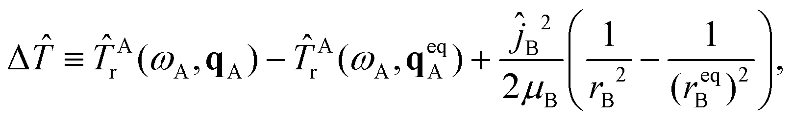
Ĥ = ![[T with combining circumflex]](https://www.rsc.org/images/entities/i_char_0054_0302.gif) rot,int(r0,ωA,ωB,Ω) + A(ωA,qA) + B(ωB,rB) + V(r0,ωA,ωB,qA,rB). rot,int(r0,ωA,ωB,Ω) + A(ωA,qA) + B(ωB,rB) + V(r0,ωA,ωB,qA,rB). | (1) |
rot,inter(r0,ωA,ωB,Ω) is the rotation-intermolecular kinetic-energy (KE) operator, the same as that given by eqn (2) of I, and is adapted from results in ref. 42. The monomer-A KE operator TA(ωA,qA) is from ref. 35 and is the sum of a vibrational term Av(qA), a rotational term Ar(ωA,qA), and a coriolis term Acor(ωA,qA). These are given, respectively, by eqn (4)–(6) of I. The monomer-B KE operator B(ωB,rB) is the sum of a rotational term Br(ωB,rB) and a vibrational term Bv(rB), which are respectively given by eqn (9) and (10) of paper I. V(r0,ωA,ωB,qA,rB) is the 9D PES of the complex. (Note that V is a function of nine coordinates, not ten, since it only depends on the difference between αA and αB.)
2.2 General procedure for computing the eigenstates of Ĥ
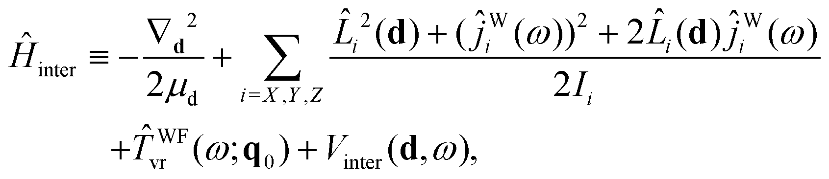
As outlined in the Introduction, Ĥ in eqn (1) is partitioned in the following four terms.24,25 The first one is the (rigid-monomer) intermolecular Hamiltonian, Ĥinter, defined as| Ĥinter(Q,Ω) ≡ rot,inter(Q,Ω) + Ar(ωA,qeqA) + Br(ωB,reqB) + Vinter(Q), | (2) |
| Vinter(Q) ≡ V(Q,qeqA,reqB) − V(Q∞,qeqA,reqB), | (3) |
The second and third terms are the two isolated-monomer Hamiltonians, ĤAv and ĤBv, in 3D and 1D, respectively, defined as
| ĤAv(qA) = Av(qA) + VA(qA), | (4) |
| VA(qA) ≡ V(Q∞,qA,reqB), | (5) |
| ĤBv(rB) = Bv(rB) + VB(rB), | (6) |
| VB(rB) ≡ V(Q∞,qeqA,rB). | (7) |
The use of the above isolated-monomer 1D potential VB(rB) in the definition of ĤBv(rB) in eqn (8) is appropriate when the monomers A and B are bound by weak vdW interactions, as in the water–CO complex.25,36 However, this choice is not optimal for HB complexes where inter-monomer interaction is stronger. Therefore, in the case of the HCl–H2O complex and isotopologues17,37,38 the 1D HCl dimer-adapted vibrational Hamiltonian was defined as
| ĤBv(rB) = Bv(rB) + VBDA(rB). | (8) |
| VBDA(rB) ≡ V(Q0,q0A,rB). | (9) |
Finally, the fourth term in Ĥ is the difference ΔĤ ≡ Ĥ − Ĥinter − ĤAv − ĤBv, which is given by
| ΔĤ(Q,Ω,qA,rB) = Δ + Acor + ΔV, | (10) |
 | (11) |
| ΔV(Q,qA,rB) = V(Q,qA,rB) − Vinter(Q) − VA(qA) − VB(rB). | (12) |
The next step is to build up the product contracted 9D basis in which to diagonalize Ĥ. We first compute the low-energy eigenstates of Ĥinter, ĤAv, and ĤBv, which are designated as |κ,J〉, |vA〉, and |vB〉, respectively. The 9D basis states are then constructed as products of the form
| |κ,J,vA,vB〉 ≡ |κ,J〉|vA〉|vB〉. | (13) |
The only part of Ĥ that has nonzero off-diagonal matrix elements in this basis is ΔĤ. It is the calculation of these matrix elements that poses the principal computational challenge.
2.3 Calculation of Ĥinter eigenstates
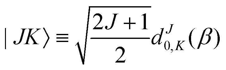
| |s,jA,kA,m,jB;JK〉 ≡ |r0,s〉|jA,kA,m〉|jB,K − m〉|JK〉. | (14) |
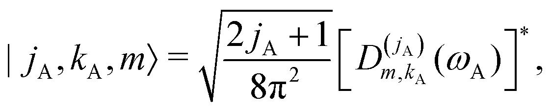 | (15) |
 denoting Wigner rotation matrix elements and jA = 0,…jmaxA. The
 | (16) |
 | (17) |
 | (18) |
For the triatom–diatom complexes investigated so far,17,25,36–38Ĥinter has been diagonalized in the basis of eqn (14) by using the Chebyshev version49 of filter diagonalization.50 The successive operation of Ĥinter on a random initial state vector that is required by this algorithm is accomplished as follows. Operation with the kinetic-energy portion of Ĥinter is effected by direct matrix-on-vector multiplication, all the relevant matrix elements having been computed prior to such multiplication. For operation with Vinter the state vector is transformed to a (r0, cosβA, γA, cosβB, (αA − αB)) grid. That representation of the vector is then multiplied by the value of Vinter at each grid point. Finally, the result is transformed back to the basis representation. A more detailed description of this procedure is given in I.
As an example, complexes such as H2O/D2O–CO and H2O/D2O–HCl belong to the molecular symmetry group G4 = [E,E*,(12),(12)*], where E* is the inversion operation and (12) permutes the H/D-nucleus coordinates of water. Therefore, the matrix of Ĥinter (and Ĥ) can, in principle, be block-diagonalized into four irreducible representations of G4. Block-diagonalization of Ĥinter with respect to parity is straightforward. As detailed in I, it is accomplished by projecting out of a random state vector that part which has either even or odd parity. That parity-filtered vector is then used as the initial state vector in the filter diagonalization procedure. Hence, the complete diagonalization of Ĥinter involves two filter diagonalization runs, one for each parity. It should be noted that the parity of an eigenstate of Ĥinter also determines the parity of each of the 9D basis functions to which it contributes, since all of the eigenstates of the intramolecular Hamiltonians ĤAv and ĤBv are symmetric with respect to E*. Thus, parity block-diagonalization of the matrix of Ĥ in the 9D basis is easily accomplished.
One important consequence of the E* symmetry of the dimers and the way in which the intermolecular basis functions transform with respect to E* is that the matrix elements of Ĥinter are all real, as proven in I. This property has been used to enhance the efficiency of the calculations, by obviating the need to work with complex-number amplitudes.
As noted above, Ĥinter and Ĥ of species like H2O/D2O–CO and H2O/D2O–HCl are also invariant with respect to hydrogen-nucleus interchange. This additional symmetry can be used to further block-diagonalize the Ĥinter matrices. Full use of G4 symmetry was made in the 9D quantum calculations of the J = 1 intra- and intermolecular rovibrational states of HCl–H2O and DCl–H2O complexes,38 because of the need to deal with considerably larger 9D basis sets relative to those used previously.
Explicit incorporation of the hydrogen-exchange symmetry into the 9D basis is somewhat more involved than making that basis parity-adapted.38 The parity of the 9D basis function |κ,J,vA,vB〉 is entirely determined by that of the intermolecular eigenstate |κ,J〉. In contrast, the symmetry of the 9D basis function with respect to the hydrogen exchange is determined by the way in which both |κ,J〉 and |vA〉 transform under this operation. The procedure by which this is handled is described in ref. 38.
2.4 Diagonalization of ĤAv and ĤBv
The eigenstates of the two intramolecular vibrational Hamiltonians, ĤAv [eqn (4)] and ĤBv [eqn (8)], are rather easy to calculate owing to their low-dimensionality, 3D and 1D, respectively for the triatom–diatom systems studied thus far.17,25,36–38 The following procedure has been employed for ĤAv (see I). A 3D product DVR basis consisting of two 1D PODVRs47,48 covering the R1 and R2 Radau coordinates, typically consisting of eight functions each, and a 1D PODVR covering the cosΘ Radau coordinate and consisting of fifteen functions, has been utilized. The matrix of ĤAv in this basis was then diagonalized by Chebyshev filter diagonalization.49
The vibrational eigenstates of ĤBv for the diatomic moiety (CO, HCl) have been computed by direct diagonalization of the matrix of that operator in a PODVR basis whose construction is described in ref. 25 and 17.
2.5 Calculation of the eigenstates of Ĥ
As mentioned previously, when diagonalizing Ĥ, the main challenge is posed by the calculation of the matrix elements of ΔĤ in eqn (39) in the 9D |κ,J,vA,vB〉 basis. This task is facilitated by taking advantage of the fact that the matrix is block diagonal in J and with respect to the parity of the basis states. The rather lengthy procedure involved in the calculation of Δ, ΔV, and Acor is presented in I (it is similar similar to the F matrix evaluation of Carrington31,51). Whenever possible, profitable use is made of the hydrogen-exchange symmetry of the dimer, that allows one to reduce the number of ΔĤ matrix-element calculations by about a factor of two.17,25,37,38
2.6 Crucial advantage of using the intermolecular eigenstates of Ĥinter in the product contracted 9D basis
It was stated already in Section 2.2 that the dimension of the final product contracted basis in eqn (13) is equal to the product of the numbers of eigenstates of each of these three lower-dimension Hamiltonians that are included in it. As emphasized in the Introduction, the main benefit of using the eigenstates of Ĥinter as the contracted basis for the intermolecular DOFs is the ease with which one can capitalize on the weak-coupling insight and include only a small number of them, with the lowest energies, in the final basis. This reduces drastically the final basis-set size, making it small enough to allow direct diagonalization of the corresponding Ĥ-matrix blocks, as illustrated by two examples below.In the case of the J = 0,1 9D calculations of H2O–CO,25 the numbers of such 5D intermolecular states, Ninter, corresponding to each of the parity/J blocks were as follows. Ninter = 60 for even/0, 52 for odd/0, 90 for even/1, and 90 for odd/1. In all the blocks, the 5D intermolecular eigenstates included in the 9D bases extended to at most 230 cm−1 above the lowest-energy state of the given parity. This is far below the intramolecular vibrational fundamentals of H2O (1600–3750 cm−1) and CO (2147 cm−1).
In addition, 21 of the lowest-energy 3D intramolecular eigenstates of ĤAv (up to 9000 cm−1 in excitation energy) and 5 of the lowest-energy 1D vibrational eigenstates of ĤBv (up to the vibrational energy of 8300 cm−1) were employed in the final 9D basis.
This resulted in the modest sized final 9D product contracted basis-sets for each of the four parity/J blocks of H2O–CO of only 6300, 5460, 9450, and 9450 for even/0, odd/0, even/1, and odd/1, respectively. These are sufficiently small to permit direct diagonalization of the corresponding Ĥ-matrix blocks.
In the J = 0 9D calculations of HCl–H2O,17 the matrix of Ĥ in the 9D basis is block diagonal in the two parity blocks. Consequently, two different sets of basis states were constructed and two different matrix diagonalizations were performed to obtain the 9D eigenstates. The blocks differ in respect to the 5D Ĥinter eigenstates, |κ〉, that were included. For the even-parity basis states 90 lowest-energy |κ〉 with even parity were included, up to 870 cm−1 above the Ĥinter ground state. For the odd-parity basis states the 90 lowest-energy |κ〉 of odd parity were included as well, covering the energy range of about 930 cm−1 above the ground state. For both parities these energies are low in comparison with the intramolecular vibrational fundamentals of H2O (1596–3650 cm−1) and HCl (2730 cm−1).
Each of these blocks was composed of the same set of H2O and H35 Cl states: the 21 lowest-energy |vA〉 and the five lowest-energy |vB〉. Hence, both blocks consist of just 9450 states, allowing their direct matrix diagonalization, as for H2O–CO above.
Thus, in the J = 0,1 9D quantum bound-state calculations of both H2O–CO and HCl–H2O complexes it sufficed to include only about 100 low-energy contracted intermolecular basis functions in the final 9D product contracted basis of dimension ∼10000, and obtain converged all intramolecular vibrational fundamentals together with low-lying intermolecular vibrational eigenstates. A primitive, uncontracted intermolecular basis would certainly be several orders of magnitude larger, making such calculations prohibitively expensive and likely impossible.
3 Theory: binary polyatomic molecule-large molecule complexes
The coordinate system described in Section 2.1, with the ẐD axis of the DF frame defined to be along the vector r0 connecting the c.m. of one monomer to that of another, is tailored for noncovalently bound complexes comprised of two small molecules, both capable of undergoing extensive internal rotations. However, this coordinate system, and the rovibrational Hamiltonian associated with it, is not appropriate for weakly bound binary complexes where one molecule is large and the other is small, and as a result the intermolecular PES shows large anisotopy while the motions of the large molecule are strongly hindered.In order to address this problem, in ref. 41 quantum bound-state methodology was formulated with molecule-large molecule complexes in mind, specifically benzene–H2O and benzene–HDO. It allows rigorous, fully coupled 9D quantum calculations of the intramolecular vibrational excitations of a flexible small molecule (H2O and HDO) weakly bound to a large molecule (benzene) taken to be rigid, together with the low-energy intermolecular vibrational states within each intramolecular vibrational manifold. The method incorporates the general approach of partitioning the vibrational Hamiltonian24,25 presented in Section 2.2. The DF frame of the complex is affixed to the large molecule (benzene), building on the previous quantum 6D (rigid-monomer) treatment of the intermolecular vibrations of benzene–H2O.52 This in turn is an extension of the earlier quantum 3D calculations of the intermolecular level structure of atom-large molecule vdW complexes53–55 (see also ref. 4 for a general discussion of this topic).
The presentation here follows that in ref. 41. It refers to the benzene–water (BW) dimer, but adapting the procedure to other molecule-large molecule complexes (e.g., those involving naphthalene or tetracene) would require relatively modest adaptations.
3.1 Vibrational Hamiltonian of the dimer
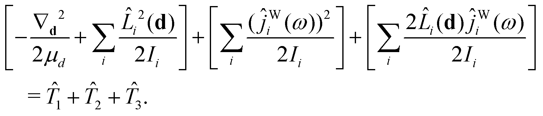
The DF frame is defined such that its origin is at the c.m. of the complex, its![[X with combining circumflex]](https://www.rsc.org/images/entities/i_char_0058_0302.gif) and Ŷ axes are parallel to the two principal axes in the plane of benzene, respectively, and its Ẑ axis is × Ŷ, perpendicular to the benzene plane. The classical nuclear KE of this system can then be written as
and Ŷ axes are parallel to the two principal axes in the plane of benzene, respectively, and its Ẑ axis is × Ŷ, perpendicular to the benzene plane. The classical nuclear KE of this system can then be written as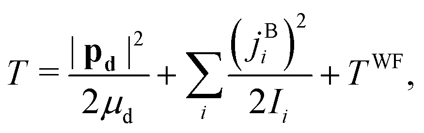 | (19) |
Starting with eqn (19) and proceeding along the lines of the development in ref. 52, the quantum vibrational Hamiltonian of the BW complex is obtained as
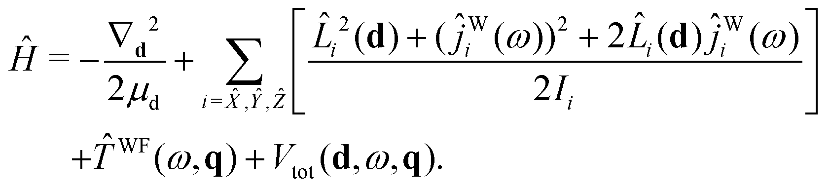 | (20) |
![[L with combining circumflex]](https://www.rsc.org/images/entities/i_char_004c_0302.gif) i is the component, measured along the ith axis, of the orbital angular momentum associated with the rotation of the c.m.s of the benzene and water moieties about the dimer c.m., and ĵWi is the operator corresponding to the component of water's angular momentum measured along the ith DF axis. WF(ω,q) is the operator associated with rotational–vibrational KE of water monomer:35
i is the component, measured along the ith axis, of the orbital angular momentum associated with the rotation of the c.m.s of the benzene and water moieties about the dimer c.m., and ĵWi is the operator corresponding to the component of water's angular momentum measured along the ith DF axis. WF(ω,q) is the operator associated with rotational–vibrational KE of water monomer:35| WF(ω,q) = WFvr(ω,q) + WFcor(ω,q) + WFvib(q). | (21) |
WFvr, WFcor, and WFvib are given in ref. 41. Finally, Vtot(d,ω,q) is the 9D PES of the benzene–water dimer, which we express as| Vtot(d,ω,q) = VB–W(d,ω,q) + VWFintra(q), | (22) |
3.2 The procedure for calculating the eigenstates of Ĥ
The coupled inter- and intramolecular vibrational eigenstates of Ĥ in eqn (20) are calculated following the general procedure described in Section 2.2 for computing the rovibrational states of noncovalently bound complexes.24,25 The difference is that in this case only one of the two monomers, the small molecule (water), is treated as flexible, while the other monomer, the large molecule (benzene), is taken to be rigid.Ĥ is partitioned into a reduced-dimension 6D (rigid-monomer) intermolecular Hamiltonian Ĥinter, a reduced-dimension 3D intramolecular vibrational Hamiltonian Ĥintra of the flexible water molecule, and a remainder term ΔĤ. From the low-energy eigenstates of Ĥinter (denoted as |κ〉, with eigenenergies Einterκ) and those of Ĥintra, (denoted as |γ〉, with eigenenergies Eintraγ) a contracted product basis |κ,γ〉 ≡ |κ〉|γ〉 is built up, which is then used to diagonalize the full 9D vibrational Hamiltonian.
Ĥ inter is defined as
 | (23) |
| Vinter(d,ω) ≡ VB–W(d,ω;q0), | (24) |
Ĥ intra is defined as
| Ĥintra ≡ WFvib(q) + Vadap(q), | (25) |
| Vadap(q) ≡ VWFintra(q) + VB–W(d0,ω0,q). | (26) |
Finally,
| ΔĤ ≡ ΔWFvr(ω,q) + WFcor(ω,q) + ΔV(d,ω,q), | (27) |
| ΔWFvr(ω,q) ≡ WFvr(ω,q) − WFvr(ω;q0), | (28) |
| ΔV(d,ω,q) ≡ VB–W(d,ω,q) − VB–W(d,ω;q0) − VB–W(d0,ω0,q). | (29) |
In the 9D |κ,γ〉 basis the matrix elements of Ĥ are thus given by
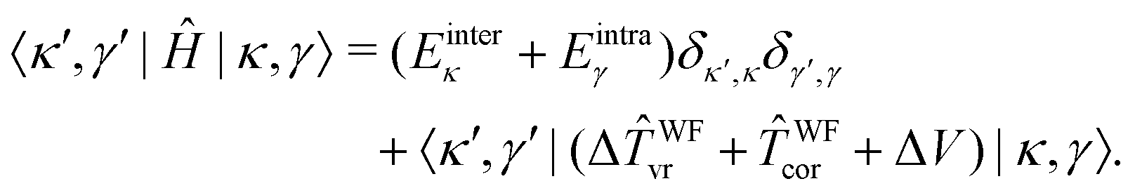 | (30) |
3.3 Coordinates and kinetic-energy operators
The coordinates on which Ĥ depends are specified in the following way. For the components of the intermolecular vector d in eqn (20) the cylindrical coordinates (dZ,ρ,Φ) are used, where dZ is the Cartesian component of d along the Ẑ axis, , and (cosΦ,sinΦ) ≡ (dX/ρ,dY/ρ), with dX and dY the Cartesian components of d along the and Ŷ axes, respectively. For the intra-water q the Radau coordinates (R1,R2,Θ)43–45 are employed. Radau bisector- z embedding is used to define the WF frame,35 as described in Section 2.1.
The kinetic-energy portion of Ĥ in eqn (20), apart from WF, can now be written as52
 | (31) |
1, 2, 3, and WF are given in Section IIC of ref. 41.
3.4 Diagonalization of Ĥinter and Ĥintra
A “cylindrical-Wigner” basis52 chosen to represent the matrix of Ĥinter consists of basis states of the form| |α,v,l,j,mj,k〉 = |dZ,α〉|v,l〉|j,mj,k〉. | (32) |
A very significant increase in computational efficiency in respect to the diagonalization of Ĥinter and, more critically, in respect to the 9D diagonalization of Ĥ, can be achieved by the symmetry factorization of the cylindrical-Wigner basis. The matrix of Ĥinter was factorized into symmetry blocks associated with the irreps of the G12 molecular symmetry group. This choice made it possible to employ the same code to handle both the H2O and HDO versions of single-sided BW complex. Details of the symmetry-factorization procure can be found in Section IID2 of ref. 41.
It should be pointed out that the same block diagonalization due to symmetry that the above accomplishes for Ĥinter carries over to the Ĥ matrix when constructed in the |κ,γ〉 representation. This is because Ĥ is invariant to the operations of G12, the |γ〉 are unaffected by those operations, and the |κ〉 transform like G12 irreps.
Ĥ inter was diagonalized by means of the Chebyshev version49 of filter diagonalization,50 which involves successive application of the operator on an initial, randomly generated state function. This operation is straightforward for the kinetic-energy portion of Ĥinter.
The operation with the potential term in eqn (23) [i.e., Vinter(d,ω)] is slightly more involved. The state function is transformed from the |α,v,l,j,mj,k〉 representation to the quadrature-grid representation |α,ρβ,Φγ,θq,ϕr,χs〉. Next, each term in the resulting grid expansion of the state function is multiplied by the value of Vinter(d,ω) at the associated grid point. Finally, the result is back-transformed to the |α,v,l,j,mj,k〉 basis.
It can be readily shown that the matrix elements of Ĥinter in the primitive basis are all real, even though the basis functions themselves are complex.41 Consequently, if the expansion coefficients in the primitive basis of the initial state function in filter diagonalization are chosen to be real initially, the analogous expansion coefficients of the state functions resulting from successive operations of Ĥinter will remain real. Working with real state vectors decreases the computational effort by about a factor of two relative to working with complex ones, and advantage was taken of that.
The eigenfunctions of Ĥintra were computed by a procedure very similar to that outlined in Section 2.4. For a given species, H2O or HDO, a primitive basis was used consisting of the product of two tridiagonal-Morse DVRs48 covering the R1 and R2 coordinates (|η1〉 and |η2〉), and a potential-optimized DVR (|η3〉) covering the Θ coordinate. In the above bases, the matrix elements of Vadap are diagonal, with each nonzero element equal to that of the potential function evaluated at the relevant 3D quadrature point. Kinetic-energy (i.e., WFvib) matrix elements were evaluated as described in Section IID of ref. 40. The intramolecular eigenvectors of Ĥintra were obtained by filter diagonalization.
3.5 Diagonalization of Ĥ
It was already mentioned in Section 3.4 that the matrix of Ĥ is block diagonal in the |κ,γ〉 basis, with the different blocks corresponding to the different irreps to which the various |κ〉 belong. In the case of benzene–H2O, for all irreps, we set Ninter = 40 and Nintra = 34. For benzene–HDO, Ninter = 40 and Nintra = 42 were employed for all irreps. For this value of Ninter, the eigenvectors of Ĥinter included in the final 9D basis extended up to at most 270 cm−1 above the ground state of Ĥinter, far below the intramolecular vibrational fundamentals of water. This resulted in the very modest sizes of the 9D symmetry-factored bases employed, Ninter × Nintra, equal to 1360 for each G12 irrep of the H2O complex and 1680 for each one of the HDO complex. It should be pointed out all of these bases are small enough to allow for direct diagonalization.Computationally, the most intensive step of diagonalizing Ĥ, the computation of matrix elements of ΔWvr, Wcor, and ΔV [eqn (30)], is described in ref. 40.
4 Theory: light polyatomic molecules inside fullerene cages
Rigorous 9D quantum treatment of the intramolecular vibrational excitations of H2O inside the fullerene C60 coupled to the low-energy intermolecular translation–rotation (TR) states was presented in ref. 40. It represents the culmination of theoretical studies over many years aimed at elucidating the quantum TR dynamics of molecules of increasing complexity (H2,56 HF,57 H2O58) nanoconfined inside fullerenes. A comprehensive review of these studies is available.59The 9D quantum methodology described here is from ref. 40.
4.1 Vibrational Hamiltonian of H2O@C60
A flexible H2O molecule encapsulated in an isolated and rigid C60 with Ih symmetry is considered. The effects of symmetry breaking57,60 on the intramolecular vibrational excitations are not included at this point. This is because the dominant contribution to this is likely to come from the dependence of the quadrupole moment of H2O on the intramolecular coordinates, which is not known.For this case, the 9D vibrational Hamiltonian of H2O@C60 can be written as
 | (33) |
,Ŷ,Ẑ) with origin at the center of the C60 cage. These axes are chosen such that Ẑ is along a C5 symmetry axis of the icosahedral cage, Ŷ is along one of the C2 symmetry axes, and = Ŷ × Ẑ. For the components of R we work with the spherical coordinates (R,β,α), with R ≡ |R|, cosβ ≡ ![[R with combining circumflex]](https://www.rsc.org/images/entities/b_char_0052_0302.gif) ·Ẑ, and (cosα,sinα) ≡ (·,·Ŷ)/sinβ. In the second group represented by ω are the three Euler angles (ϕ,θ,χ) that fix the orientation of the water moiety's molecule-fixed (MF) axis system relative to the CF frame. In the third group represented by q are the three vibrational coordinates of the water moiety, for which the Radau coordinates (R1,R2,Θ)43–45 were chosen. Radau bisector-z embedding35 is used to define the water MF frame, as described in Section 2.1.
·Ẑ, and (cosα,sinα) ≡ (·,·Ŷ)/sinβ. In the second group represented by ω are the three Euler angles (ϕ,θ,χ) that fix the orientation of the water moiety's molecule-fixed (MF) axis system relative to the CF frame. In the third group represented by q are the three vibrational coordinates of the water moiety, for which the Radau coordinates (R1,R2,Θ)43–45 were chosen. Radau bisector-z embedding35 is used to define the water MF frame, as described in Section 2.1.
In eqn (33), going from left to right, the terms in Ĥ correspond respectively to the KE of the c.m. translational motion of the water, the vibration-rotation KE of the water (vr), the Coriolis contribution to the KE of the water (cor), the vibrational KE of the water (v), and the 9D PES of flexible H2O inside C60 (Vtot). The explicit forms of vr, cor, and v, from ref. 35, are given by eqn (3)–(5) of ref. 40. Vtot is expressed as the sum of a water–cage interaction term, VH2O–cage, and an isolated-water term, Vintra:
| Vtot(R,ω,q) = VH2O–cage(R,ω,q) + Vintra(q). | (34) |
4.2 Computing the eigenstates of Ĥ
The overall approach to calculating the coupled intramolecular and TR eigenstates of Ĥ in eqn (33) is similar to that described in Section 3.2 for binary molecule-large molecule complexes.41 This is natural, as in both cases the large molecule, benzene or C60, is taken to be rigid, while the water molecule is treated as flexible.Following the well-established general procedure24,25 outlined already in Sections 2.2 and 3.2, Ĥ is partitioned into three parts, in the following way. The first part is a 6D intermolecular Hamiltonian Ĥinter, with the eigenfunctions |κ〉 and eigenvalues Einterκ. It is defined as
 | (35) |
| Vinter(R,ω) = VH2O–cage(R,ω,q0). | (36) |
The second part is a 3D intramolecular Hamiltonian Ĥintra (of the water molecule), with the eigenfunctions |γ〉 and eigenvalues Eintraγ. It is defined as
| Ĥintra(q) ≡ v(q) + Vadap(q), | (37) |
| Vadap(q) ≡ Vintra(q) + VH2O–cage(R0,ω0,q). | (38) |
From the above 6D and 3D reduced-dimension eigenfunctions a 9D contracted product basis is constructed composed of functions of the form |κ,γ〉 ≡ |κ〉|γ〉 and then used to diagonalize the full Ĥ.
This leaves a 9D remainder term ΔĤ. From eqn (33) and the definitions of eqn (35) and (37), one has
| ΔĤ(R,ω,q) = Δvr(ω,q) + ΔV(R,ω,q) + cor(ω,q), | (39) |
| Δvr(ω,q) = vr(ω,q) − vr(ω;q0), | (40) |
| ΔV(R,ω,q) ≡ VH2O–cage(R,ω,q) − VH2O–cage(R,ω;q0) + Vintra(q) − Vadap(q). | (41) |
In the |κ,γ〉 basis, the matrix elements of Ĥ are given by
 | (42) |
4.3 Diagonalizing Ĥinter and Ĥintra
Ĥ inter is diagonalized in a primitive basis composed of functions of the form| |n,l,ml,j,mj,k〉 = |n,l,ml〉|j,mj,k〉, | (43) |
 | (44) |
The same type of symmetry factorization is employed in Section 4.4 to block diagonalize Ĥ in the |κ〉|γ〉 basis. This is possible because the |κ〉 have well-defined symmetry with respect to the p2π/5 Ẑ-axis rotations and Ĥ is invariant with respect to them.
The other symmetry used to block diagonalize the Ĥinter matrix (and that of Ĥ) further is parity, the symmetric or antisymmetric transformation of states due to inversion of the coordinates of the water particles though the CF origin. The states of the intermolecular basis transform upon inversion, Ê*, as
 | (45) |
The eigenstates of Ĥintra [eqn (37)] were calculated as outlined in Section 3.4, utilizing a product basis of three 1D DVR functions covering each of the vibrational (Radau) coordinates.40Ĥintra was diagonalized by using the Chebyshev version of filter diagonalization.
4.4 Diagonalization of Ĥ
Having computed the inter- and intramolecular eigenstates, the symmetry-adapted 9D bases |κ,γ〉, in which Ĥ is diagonalized, are constructed by including the thirty-four lowest-energy intramolecular states, |γ〉, corresponding to ΔEintra ≤ 11300 cm−1, and all intermolecular states, |κ〉, with the appropriate symmetry having ΔEinter ≤ 410 cm−1 (far below the intramolecular vibrational fundametals of H2O). Appropriate symmetry refers to the way in which the |κ〉 transform with respect to (a) the operations of Ih and (b) the specific C5 operations corresponding to rotations about the Ẑ axis. Owing to the extensive symmetry factorization, the final 9D symmetry-adapted basis-set sizes are very small, ranging from 34 (Au) to 816 (Hg), depending on the irrep, as shown in Table IV of ref. 40.
Moreover, since the 9D basis sets shown in this table include Nintra = 34 intramolecular states |γ〉 for all symmetry blocks, the number of intermolecular states |κ〉 (Ninter) in the 9D basis is obtained by dividing the basis-set size for each symmetry block in Table IV (ref. 40) by 34. One finds that Ninter ranges from 1 for the Au irrep to 24 for the Hg irrep. It is these very small values of Ninter, made possible by (a) the efficient exploitation of the weak coupling between the intra- and intermolecular vibrational DOFs and (b) symmetry factorization, that account for the small sizes of the 9D basis sets.
The most demanding task in diagonalizing any of the symmetry blocks of Ĥ in the 9D basis is to compute the matrix elements of ΔĤ [eqn (39)], given by
 | (46) |
Given the small sizes of the 9D symmetry blocks of the Ĥ matrix, their eigenstates are obtained by diagonalizing each of them directly.
5 Applications
5.1 HCl–H2O complex and isotopologues
Mixed (HCl)n(H2O)m clusters have long been of interest to experimentalists and theorists alike,64 owing to the role these complexes play in atmospheric chemistry, ozone depletion in particular. In addition, small HCl–water clusters provide a microscopic view of the steps that ulimately result in the dissociation of HCl in bulk water.64,65The HCl–H2O binary complex, the smallest of (HCl)n(H2O)m clusters, is of considerable significance in its own right. It has been the subject of numerous high-resolution spectroscopic studies, including microwave spectroscopy,66,67 ragout-jet FTIR68,69 and infrared (IR) cavity ringdown spectroscopy70 in the gas phase, and IR spectroscopy in liquid helium, as well as in nanodroplets.71–75 The vibrational predissociation dynamics of the HCl–H2O dimer following excitation of the HCl stretch have been studied as well,76,77 leading to the first determination of the dimer dissociation energy D0 = 1334 ± 10 cm−1.76
Theoretical studies of HCl–H2O dimer over the years78–82 have established that the equilibrium, minimum-energy structure has a near-linear hydrogen bond with HCl serving as the proton donor to the O atom of water which is the proton acceptor. This global minimum is non-planar, and one of its two symmetrically equivalent pyramidal Cs structures is shown in Fig. 1.
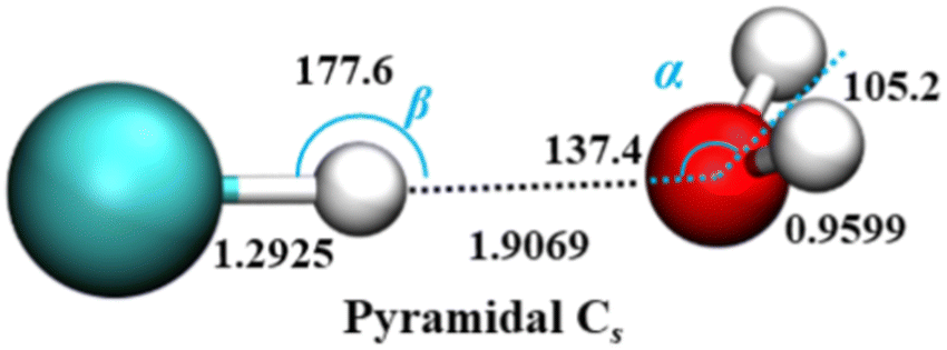 | ||
| Fig. 1 Equilibrium geometry of the HCl–H2O complex (distances in Å and angles in deg.), on the ab initio calculated PES-2021 (ref. 17). α presents the angle between H–O (H in HCl) vector and C2 axis of H2O. H, Cl, and O atoms are depicted as white, green, and red, respectively. | ||
Mancini and Bowman83 developed the ab initio based 9D PES of this complex, constructed by means of a permutationally invariant fit to over 44000 CCSD(T)-F12b/aug-cc-pVTZ configurations and energies, with the overall root-mean-square error (RMSE) of 24 cm−1. Hereafter, this PES is referred to as PES-2013. Quantum diffusion Monte Carlo (DMC) calculations performed on this PES83 gave for the dimer's dissociation energy (D0) the value of 1348 ± 3 cm−1, in good agreement with the experimental result.76 The vibrationally averaged ground-state geometry of HCl–H2O was also characterized.
Until recently, no rigorous, high-dimensional quantum calculations of excited intra- and intermolecular vibrational states of the HCl–H2O dimer were reported. This motivated the theoretical study presented in ref. 17, that had two objectives. The first one was to report a new full-dimensional (9D) PES for this dimer, denoted hereafter as PES-2021. The methodology utilized in its construction is similar to that utilized to generate the 9D PES for the H2O–CO interaction.84 The HCl–H2O PES-2021 is based on circa 43000 data points computed at the level of CCSD(T)-F12a/aug-cc-pVTZ with the basis-set-superposition-error (BSSE) correction. The ab initio points are fit using the ultraflexible permutation invariant polynomial-neural network (PIP-NN) approach,85–87 with the RMSE of only 10.1 cm−1.
The second objective of this paper was to present the results of the first fully coupled 9D quantum calculations of the intra- and intermolecular vibrational states of the HCl–H2O dimer. PES-2021 and the bound-state methodology described in Section 2 were employed. The 9D calculations yielded the three intramolecular vibrational fundamentals of the H2O moiety and the stretch fundamental of the HCl subunit, as well as their frequency shifts from the gas-phase monomer values, together with the low-energy intermolecular vibrational states of the complex within each intramolecular vibrational manifold. These and other theoretical results were compared with the available experimental data.
The binding energy D0 of the complex calculated in 9D on PES-2021 is 1334.63 cm−1 (and 1336.66 cm−1 in 5D), which agrees extremely well with the experimental D0 value of 1334 ± 10 cm−1.76 Thus, for this quantity, PES-2021 yields better agreement with experiment than the PES by Mancini and Bowman,83 for which DMC calculations gave D0 = 1348 ± 3 cm−1. Since the global minimum of PES-2021 is at −1878.2 cm−1, the 9D ZPE of the HCl–H2O dimer is 543.6 cm−1.
The effective, vibrationally averaged ground-state geometry of the HCl–H2O complex has been the subject of considerable attention.66,67,83 The PES of the complex has two symmetrically equivalent global minima, one of which is depicted in Fig. 1, corresponding to a nonplanar, pyramidal equilibrium geometry with Cs symmetry. These two minima are separated by a barrier with the height of only 49 cm−1. This suggests the possibility of the ground-state wave function delocalization over the double-well minimum of the complex, which would result in an effective C2v geometry. In fact, the DMC calculations on PES-2013 did show the hydrogen atoms of the H2O moiety as delocalized across the two global minima, resulting in a vibrationally averaged planar C2v geometry.83
However, the calculations on PES-2021 arrived at a different conclusion.17 There, the degree of nonplanarity of H2O moiety is described by βA, the water polar angle between the C2 axis of H2O and the vector r0 connecting the c.m. of H2O to that of HCl. To within a small fraction of a degree, βA is the complement of the angle α in Fig. 1. For any eigenstate of HCl–H2O, the expectation value of βA, 〈βA〉, is calculated as 〈βA〉 = cos−1〈cosβA〉, where 〈cosβA〉 is the expectation value of cosβA for a given state.
In the ground state of the complex, 〈βA〉 = 33.80°, which implies that on PES-2021 the vibrationally averaged ground-state geometry of the HCl–H2O complex is distinctly nonplanar. Moreover, the calculated 〈βA〉 of 33.80° agrees remarkably well with the experimentally determined value of 34.7° for this out-of-plane bend angle (denoted ϕ).67
The intermolecular vibrational states calculated in this study are assigned to the fundamentals, first and second overtones, and combinations of the following three intermolecular modes: (1) the inversion mode, νinversion, at 85.00 cm−1 (9D), which corresponds to the large-amplitude motion (rotation) of the H2O moiety about the A axis (its a principal axis). (2) The intermolecular stretch mode, νstretch, at 132 cm−1 (9D). (3) The water rock mode, νrock, at 146 cm−1 (9D), corresponding to the rotation of the H2O moiety about the out-of-plane ŷA axis (its c principal axis).
These assignments, for this complex and others, are made in part by inspecting contour plots of the reduced probability densities (RPDs) associated with the water-c.m.-to–HCl-c.m. vector r0 for each in suitably chosen coordinates. For example, Fig. 2 shows such plots for the ground state and three members of the inversion-mode progression: νinversion, 2νinversion, and 3νinversion. Clear nodal patterns make it easy to count the number of quanta in the inversion mode. The contour plot of the RPD of the ground state, in the top left panel of Fig. 2 exhibits two prominent symmetrically placed maxima of the same magnitude, associated with the two equivalent nonplanar vibrationally averaged ground-state geometries of HCl–H2O having 〈βA〉 = 33.80°.
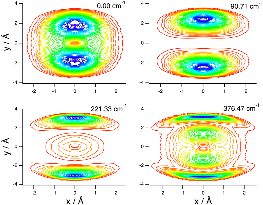 | ||
| Fig. 2 Contour plots of the reduced probability densities, as a function of the coordinates x and y defined in the text, of the ground state of HCl–H2O (top left) and the following inversion states: (top right) νinversion, (bottom left) 2νinversion, and (bottom right) 3νinversion. Reproduced from ref. 17 with permission from the PCCP Owner Societies. | ||
A complementary way of making the assignments is by inspecting how the expectation values, and the corresponding root-mean-square amplitudes, of judiciously chosen coordinates vary from one state to another. These quantities tend to be sensitive indicators of the excitation, or lack thereof, of certain vibrational modes. Less essential, but also helpful, for the assignments are the quantities which we refer to as the basis-state norm (BSN). They measure the contribution of the dominant product inter/intra-basis state to the given full-dimensional eigenstate. A BSN value close to 1 means that the eigenstate is highly “pure”, i.e., dominated by a single inter/intra-basis state.
The large-amplitude water inversion mode stands out for its strong negative anharmonicity. In the inversion mode progression, the states νinversion, 2νinversion, and 3νinversion have energies of 85.0, 217.29, and 382.04 cm−1, respectively. Clearly, the energy differences between the neighboring inversion states grow with the increasing number of quanta. The other intermolecular modes show weak positive anharmonicity.
Concerning the the intramolecular vibrational frequency shifts of the monomers in the HCl–H2O complex, the HCl stretch frequency shift (redshift) from the 9D calculations (Δν9D), −157.9 cm−1, is rather large due to hydrogen bonding with H2O, and agrees very well with the measured HCl stretch redshift in the complex of −161.9 cm−1.68,70 In contrast, the 9D frequency shifts (Δν9D) of the H2O vibrational modes are small. The water stretches ν1 and ν3 exhibit redshifts of −5.50 and −2.61 cm−1, respectively. The water bend ν2 and its overtone 2ν2 are blueshifted by +3.43 and 9.58 cm−1, respectively. The small magnitude of the frequency shifts of the vibrational modes of H2O in comparison to the large redshift of the HCl stretch is readily understood. In the dimer, the O atom of H2O is the proton acceptor, and the two H atoms are free, not involved in the hydrogen bonding with HCl. Consequently, the H2O vibrations are only weakly perturbed by HCl, resulting in their small frequency shifts.
Unfortunately, experimental data are lacking for comparison with the above theoretical results for the H2O vibrational frequency shifts. The O–H stretching vibrations of HCl–H2O fall in the highly congested spectral region, where they overlap with the vibrations of pure water clusters.69 This makes their reliable assignment very difficult and precludes definitive comparison with theory.
The quantum 9D calculations in ref. 17 also reveal the appreciable effects that the excitation of different intramolecular modes has on the intermolecular vibrational states of HCl–H2O. The large-amplitude inversion mode νinversion is the most sensitive, as the excitation of any of the intramolecular modes changes its energy relative to that in the ground intramolecular vibrational state by 6–16 cm−1. Not surprisingly, the intermolecular vibrational modes of (primarily) the H2O moiety couple most strongly to the intramolecular νHCl mode. Its excitation causes the largest changes in the energies of the intermolecular vibrational modes: the νinversion energy decreases by 16.3 cm−1, that of νstretch increases 5.6 cm−1, and the energy of the νrock mode increases by 18.5 cm−1.
In ref. 37, the full-dimensional and fully coupled quantum calculations of the inter- and intramolecular vibrational states performed previously for HCl–H2O (HH)17 were extended to three additional isotopologues of the hydrogen chloride–water complex: DCl–H2O (DH), HCl–D2O (HD), and DCl–D2O (DD). Their purpose was to elucidate the isotopologue variations of a range of bound-state properties of the hydrogen chloride–water complex, and compare them to those of the HH complex. The results largely mirror those obtained for the HH complex.17 But, the energies of νinversion and νrock, which primarily involve the motions of the water moiety, are particularly sensitive to the deuteration of H2O, much more so than the νstretch. This results in the reversal of the energy ordering of the νrock and νstretch fundamentals in the HD and DD complexes, relative to that in the HH and DH complexes. The DCl stretch frequency shift (redshift) computed in 9D for the DD complex, −114.91 cm−1, is in excellent agreement with the corresponding experimental value of −115.20 cm−1.70
In the same paper,37J = 1 rovibrational states of the four isotopologues were computed in the rigid-monomer approximation, allowing the calculation of the principal rotational constants of the complexes for a given vibrational state. For all isotopologues, calculated and measured67 values of the ground-state B and C rotational constants differ by about 1%, well within the uncertainty introduced by taking the monomers to be rigid in the analysis of the experimental data.
Fully coupled 9D quantum calculations of the J = 1 intra- and intermolecular rovibrationals states of HCl–H2O and DCl–H2O were reported in ref. 38, complementing the previous J = 0 9D calculations.17,37 They revealed significant variations of the energy differences between the K = 1 and K = 0 eigenstates with the intermolecular rovibrational states, for which a qualitative explanation was given.
5.2 H2O–CO, D2O–CO, and HDO–CO complexes
The interactions of water with other molecules are of great fundamental and practical significance. This has motivated spectroscopic and theoretical studies of numerous binary water-containing complexes. H2O–CO, and its isotopologues, figures prominently among them, since both constituent species are abundant in the atmosphere and of utmost importance. Water and CO are encountered, in weakly bound complexes and as collision partners, in a variety environments, including Earth's atmosphere, as the products of combustion reactions, in the interstellar medium, as well as in the coma of comets and in protoplanetary disks.88–90 Due to its ubiquity, the water–CO complex has been in the focus of numerous high-resolution spectroscopic investigations, including microwave spectroscopy,91,92 and IR spectroscopy in the regions of the C–O stretch,93 the O–H stretch,94 the D2O bend,95 and the H2O bend.89 The most recent IR spectroscopic measurements96 have probed the C–O stretch regions of H2O–CO, D2O–CO, and HOD–CO, and the O–D stretch regions of D2O–CO, HOD–CO, and DOH–CO.From these studies, it emerged that the equilibrium structure of the water–CO complex is planar, with the heavy atoms arranged in a roughly collinear configuration and a hydrogen bond between the water moiety and the C atom of the CO; the CO bond axis is almost parallel to the intermolecular axis connecting the centers of mass of the two monomers. In addition, there is a local minimum in which the O atom of CO points towards the hydrogen atoms of the water molecule. All observed spectroscopic transitions are doubled, indicating the large-amplitude tunneling motion of the water molecule within the complex that exchanges the free and the bound hydrogen atoms in the intermolecular bond. This gives rise to two tunneling states with different symmetry along the tunneling coordinate, the spatially symmetric state A and the spatially antisymmetric B state. Both H2O and D2O have two identical particles, H with the nuclear spin 1/2 (a fermion) and D with with the nuclear spin 1 (a boson), respectively. The Pauli principle requires that the total molecular wave function, i.e., its spatial and nuclear-spin components, must be antisymmetric with respect to the exchange of the two fermionic H nuclei of H2O, and symmetric with respect to the exchange of the two bosonic D nuclei of D2O. This requirement leads to a particular entanglement of the spin and spatial quantum states. In the case of H2O–CO, the symmetric tunneling state A correlates with para-H2O (total nuclear spin I = 0, antisymmetric spin function) while the antisymmetric B state correlates with ortho-H2O (total nuclear spin I = 1, symmetric spin function). Since D nuclei are bosons, the situation is reversed for D2O–CO, and its A state correlates with ortho-D2O (total nuclear spin I = 0,2, symmetric spin functions) and B with para-D2O (total nuclear spin I = 1, antisymmetric spin function). Excitation of certain intramolecular modes in H2O–CO93 and D2O–CO95 was found to affect measurably the magnitudes of the tunneling splittings, relative to those in the ground vibrational state of the complexes. The tunneling splittings are also known to depend strongly on the quantum numbers K = 0 and 1.96
Complete description of the multidimensional and strongly coupled intra- and intermolecular rovibrational dynamics, including tunneling, of water–CO complexes requires a full-dimensional and fully coupled quantum treatment. A prerequisite for this is an accurate 9D PES, which was not available until recently. Various 5D and 6D PESs were developed, starting from ab initio calculations followed by morphing to achieve improved agreement with experiment.89 These PESs were used in the quantum 5D calculations of the intermolecular rovibrational levels. The latest 5D (rigid monomer) intermolecular PES for H2O–CO computed at a higher level of ab initio theory by Kalugina et al.90 was utilized in J = 0,1 bound-state and scattering calculations. The same 5D PES was employed by Barclay et al.96 in the quantum bound-state calculations of the J = 0–2 rovibrational levels of H2O–CO and D2O–CO. None of these calculations could include the coupling between the inter- and intramolecular vibrations.
The situation changed with the publication of the first full-dimensional (9D) PES for the H2O + CO system by Liu and Li,97 hereafter referred to as the LL PES. This PES is based on ∼102000 points calculated at the level of an explicitly correlated coupled-cluster method with single, double, and perturbative triple excitations with the augumented correlation-consistent polarized triple zeta basis set (CCSD(T)-F12a/AVTZ), using the permutation invariant polynomial-neural network (PIP-NN) method.
Combined with the methodology in Section 2, the LL PES was utilized for the 9D quantum J = 0,1 rovibrational bound-state calculations of H2O–CO and D2O–CO in ref. 25, that covered the intramolecular rovibrational excitations of the monomers, together with the low-energy intermolecular rovibrational states of the complexes within each intramolecular vibrational manifold.
For H2O–CO and D2O–CO in their ground states, the 9D computed K = 1 hydrogen-exchange tunneling splittings, −0.228 and −0.016 cm−1, respectively, are significantly smaller by magnitude than those obtained for K = 0 (0.727 and 0.027 cm−1, respectively), consistent with the 5D rigid-monomer results in the literature (for a different PES).96 However, the actual magnitudes of the tunneling splittings from 9D and 5D (rigid-monomer) calculations differ appreciably. Although the individual K = 0 and K = 1 splittings cannot be measured directly, the sums of their absolute values are measurable, with the experimental values of 1.1130 and 0.0676 cm−1 for H2O–CO and D2O–CO, respectively.92 The 9D calculated sums of K = 0 and K = 1 splittings are 0.955 and 0.043 cm−1, meaning that they are smaller than the measured values by about 14% for H2O–CO and 36% for D2O–CO.
The K = 0 tunneling splittings were computed in 9D also for the intramolecular vibrational fundamentals of the monomers in H2O–CO and D2O–CO. The results showed that they are sensitive to the intramolecular vibrational excitation. Thus, for H2O–CO, excitation of any of the intramolecular fundamentals of H2O decreases the magnitude of the tunneling splitting relative to that in the ground state, by up to 23% for the ν1 mode.
The 9D calculations allowed a detailed analysis of the frequency shifts (Δν9D) of the intramolecular vibrational modes of the two complexes. In H2O–CO, the H2O bend mode ν2 (and its overtone) and the CO stretch are blueshifted, by about 4 and 11 cm−1, respectively, relative to the values calculated for the isolated monomers. The corresponding experimental values are 3.889 and 10.3 cm−1,93,96 respectively. For D2O–CO, the blueshifts calculated for the ν2 the CO stretch modes are about 3.5 and 12.4 cm−1, respectively, similar to the corresponding blueshifts computed for H2O–CO. The agreements with the experimental results, about 2.295 and 11 cm−1,96 respectively, is very good.
Unlike the ν2 and νCO modes, the 9D computed water stretching modes ν1 and ν3 are redshifted in both H2O–CO and D2O–CO, the ν1 mode much more in magnitude than the ν3 mode, −17 and −3 cm−1, respectively, for H2O–CO. This agrees qualitatively with the available experimental redshifts for these modes,94,96 but the quantitative agreement is not as good as for the water bend mode and the CO stretch. Given that the calculations are rigorous and highly converged, these discrepancies must reflect certain deficiencies of the water–CO PES.
In ref. 36 the 9D quantum calculations of the J = 0,1 rovibrational states were extended to the HDO–CO complex, using the same methodology of Section 2. Unlike the two isotopically symmetric isotopologues, H2O–CO and D2O–CO, the isotopically asymmetric HDO–CO does not exhibit hydrogen-interchange tunneling, since the H and D atoms are distinguishable.
While quenching the tunneling splitting, the presence of the distinguishable H and D atoms gives rise to two isomers, the D-bonded HOD–CO and the H-bonded DOH–CO. Their origin is entirely quantum mechanical, as the two (symmetrically equivalent) minima on the PES of the complex associated with each of the isomers have identical well depths. Based on the relative intensities of the spectra of these two isomers, the energy difference between their ground states was estimated93 to be 12.4 ± 2.5 cm−1.
The 9D calculations revealed that the eigenstates of the D-bonded and H-bonded isomers, designated as D and H respectively, can be readily distinguished in two ways, based on the expectation values of the distances of the D and H atoms of HDO to the C atom of CO, and by inspecting the contour plots of the RPDs of the eigenstates. The latter show that almost all excited intermolecular vibrational states of HDO–CO up to about ΔE = 160 cm−1 are completely localized in either the D-bonded or H-bonded potential minimum, allowing their unambiguous assignment as D or H isomers.
This is evident from Fig. 3. Its left column displays the contour plots of the RPDs of the four lowest-energy J = 0 D states, while the RPDs of the corresponding H states are in the right column.
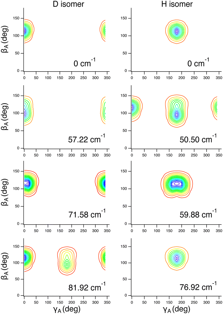 | ||
| Fig. 3 Contour plots of the reduced probability densities (RPDs), as a function of the Euler angles γA and βA, of the four lowest-energy J = 0 intermolecular vibrational states of the D-bonded (D) and H-bonded (H) isomers of HDO–CO, from 5D calculations. The energies shown are relative to those of J = 0 D/H ground states. The two topmost panels display the RPDs of the D and H ground states, peaking at, and localized around, γA = 0° and γA = 180°, respectively. The next three panels show the RDPs of the first three excited D and H intermolecular states. The D state at 81.92 cm−1 and the H state at 50.50 cm−1 are delocalized over both minima as a result of accidental near-degeneracy. For additional discussion, see the text. Reprinted with permission from ref. 36. Copyright 2022 American Chemical Society. | ||
The coordinate that differs the most for the two isomers is the Euler angle γA of HDO, which refers to the rotation about the water ẑA axis (Section 2.1). The D-bonded isomer has γA values near 0°, while for the H-bonded isomer γA values are near 180°. For this reason γA is on the horizontal axis of the panels in Fig. 3. On the vertical axis is βA, the Euler angle between the ẑA axis of the water molecule and the inter-monomer vector connecting the c.m. of A to that of B. Its values are similar for the two isomers.
Concerning the two isomer-mixed low-energy exceptions evident in Fig. 3, the states in question are at nearly the same energy relative to the D ground state. From the 9D quantum calculations, the ground-state energy of the H-bonded isomer is 30.6 cm−1 higher than that of the D-bonded isomer. The main contribution to the energy difference comes from the potential energy. In the ground state of the D-bonded isomer, the expectation value of the potential energy is about 22 cm−1 smaller than that for the ground state of the H-bonded isomer, corresponding to about 70% of the total energy difference. The experimental estimate93 of the energy gap between the two isomers is 12.4 ± 2.5 cm−1. Therefore, experiment and theory agree, although not perfectly, about the small energy separation between the two isomers.
The D- and H-bonded isomers exhibit the same trends in the calculated frequency shifts of the intramolecular vibrational modes. They also agree qualitatively with what was observed in the calculations regarding the frequency shifts for H2O–CO and D2O–CO25 discussed previously. In both isomers, the HDO bend mode ν2 and the CO stretch νCO are blueshifted relative to the values calculated for the isolated monomers, that for the CO stretch being appreciably larger than the blueshifts of the HDO bend fundamental. In contrast, the HDO stretching modes νOD and νOH of both isomers are redshifted. As expected, the νOD redshift is much larger in the D-bonded isomer than in the H-bonded isomer. Conversely, the νOH redshift is much larger in the H-bonded isomer than in the D-bonded isomer.
The redshifts calculated for the νCO mode of the D- and H-bonded isomers are 12.0 and 11.6 cm−1, respectively. They compare well with the corresponding experimental values96 of 11.2 and 10.5 cm−1, respectively. Comparison with experiment is possible also for the νOD mode of the two isomers. The calculated redshifts are −12.0 (D) and −0.8 cm−1 (H), respectively, while the respective measured values are −14.2 and +1.8 cm−1.96 Experimental frequency shifts are not available for the other modes HDO–CO.
5.3 Benzene–H2O and benzene–HDO complexes
Numerous spectroscopic studies have been directed at benzene–H2O and benzene–HDO complexes.98–104 A major impetus for them was the realization that benzene–H2O and benzene–HDO are highly nonrigid, which emerged first from the matrix isolation study.105 Their fluxional character was characterized more precisely by the subsequent microwave98,99 and IR spectra.101,103 The picture that emerged from these studies has the vibrationally averaged position of the c.m. of the water molecule on the C6 axis of benzene, with both hydrogens oriented preferentially towards the ring, in the π hydrogen-bonding configurations. The water molecule undergoes multiple intermolecular large-amplitude motions (LAMs) already in the ground vibrational state, in particular the internal rotation about the sixfold axis, and the facile in-plane torsional (or rocking) motion that exchanges its two H atoms, in such a way that, on the vibrationally averaged basis, the complex retains the sixfold symmetry of the benzene ring. In benzene–HDO, HDO preferentially forms the π hydrogen bond via the D atom.102,105The low-energy intermolecular levels also give rise to a number of transitions in the OH stretch region of the IR spectrum, that in the absence of the LAMs would be negligibly weak.101,103 The features arising from the LAMs are present in the Raman spectra of benzene–H2O as well, as four prominent intermolecular bands in the low-energy region below 60 cm−1.100
Concerning theoretical treatments, three 6D (rigid-monomer) quantum calculations of the LAMs of benzene–H2O were reported.52,106,107 One of them was a ground-state diffusion Monte Carlo simulation.107 In the quantum 6D approach of Linse,106 the intermolecular vibrational levels of rigid H2O were calculated inside the external potential of benzene molecule, but assuming that benzene is infinitely heavy, thereby leaving out a great deal of angular momentum coupling present in the complex. Only the quantum 6D calculation of the intermolecular vibrational states of benzene–H2O by Kim et al.52 was dynamically rigorous.
A quantitative treatment of the vibrational level structure of benzene–H2O/HDO capable of accounting for the combination bands prominent in the measured IR and Raman spectra as well as the OH-stretch vibrational frequency shifts can be achieved only by fully coupled 9D quantum bound-state calculations for flexible H2O and rigid benzene, extending to the energies of the H2O vibrational fundamentals and overtones.
The methodology for such a rigorous quantum treatment was presented in ref. 41; it is described in Section 4. In the absence of an ab initio calculated 9D PES of the benzene–water dimer, the PES employed in these calculations was constructed by combining the atom–atom pairwise-additive benzene–water interaction potential from Karlström et al.108 with the 3D PES for the isolated, gas-phase water molecule from Mizus et al.109
The 9D quantum bound state calculations and the simulations of the IR and Raman spectra (the latter using the methodology also introduced in ref. 41) have revealed numerous interesting facets of the highly quantum behavior of the H2O and HDO complexes. Thus, plots of the probability density functions show that in the ground intermolecular state of the H2O complex, both H atoms of water interact equivalently with the benzene, as deduced experimentally.98,105 For the HDO complex, the same plots show that only the D nucleus is localized close to the benzene plane while the H atom is further away, in accord with the experimental observations.102,105
Based on the 9D quantum calculations, the stretching modes of H2O (ν1 and ν3) and HDO (νOD and νOH) are redshifted, while the H2O/HDO bend fundamentals (ν2) and overtones (2ν2) are blueshifted, relative to the ones calculated for the respective isolated monomers. For the ν1 and ν3 modes of H2O and the νOH mode of HDO, the prediction of their redshift agrees with the experimental results,103 but the redshift magnitudes are roughly a factor of two smaller than the corresponding experimental values. In addition, calculations provide rich data about the effects that the excitation of various intramolecular modes of H2O and HDO has on the LAM low-frequency intermolecular states of the two dimers.
The comparison between theory and experiment is the most complete when contrasting the simulated and measured IR103 and Raman100 spectra of the dimers. The dominant bands in the computed IR spectra of the H2O complex in the OH-stretch region, shown in Fig. 4, are in excellent agreement with the experimental results and analysis of Pribble et al.,103 regarding the relative band positions and band assignments. On the other hand, a number of smaller-intensity bands cannot be assigned with confidence to particular features in the spectra, reflecting the limitations in the accuracy of the PES.
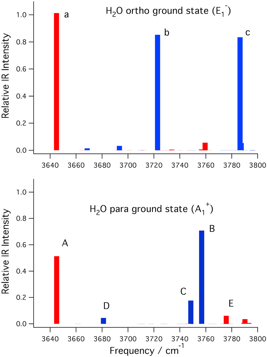 | ||
| Fig. 4 Calculated infrared spectra in the region of the OH stretching fundamentals of benzene–H2O. Top: Initial state is the ortho ground state. Bottom: Initial state is the para ground state. In both spectra red bars signify parallel bands and blue bars signify perpendicular bands. For more information see ref. 41. Reproduced from ref. 41, with the permission of AIP Publishing. | ||
In the case of the HDO complex, while the IR spectrum computed in the region of the OH stretch does not match quantitatively with the measured spectrum,103 it agrees with it in a number of important features, allowing its tentative interpretation after making some reasonable assumptions about the energies of a couple of intermolecular modes.41
Further, more quantitative theoretical treatment must await the development of an accurate ab initio 9D PES. Once at hand, the bound-state and spectroscopic calculations on it utilizing the methods in ref. 41 will allow a definitive interpretation of the wealth of the IR and Raman spectroscopic data available for the benzene–H2O and benzene–HDO complexes.
5.4 Flexible H2O molecule in C60
H2O@C60 is a fascinating endohedral complex where a polar molecule, H2O, is encapsulated inside a highly symmetric, nonpolar interior of C60, as depicted in Fig. 5. It belongs to the family of light-molecule endofullerenes (LMEFs), that have molecules such as H2, HF, and CH4, characterized by small masses and large rotational constants, encapsulated inside the cages of C60, C70 and other fullerenes.59,110 These inclusion compounds have all been synthesized111–114 utilizing the approach known as molecular surgery.115–117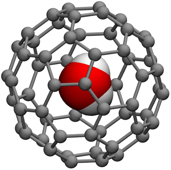 | ||
| Fig. 5 Schematic depiction of the molecular structure of H2O@C60. Reproduced from ref. 40, with the permission of AIP Publishing. | ||
The spectroscopy and dynamics of guest molecules in H2O@C60 and other LMEFs are dominated by nuclear quantum effects (NQEs),59,110,118 especially for the low temperatures (typically ranging from 1.5 K to about 30 K) at which the spectroscopic measurements are usually carried out. The NQEs arise from a combination of quantization of the translational c.m. DOFs of the encapsulated molecules due to their confinement and widely spaced quantized rotational states of the light molecules. In addition, in the case of H2O as outlined in Section 5.2, satisfying the Pauli principle gives rise to two nuclear spin isomers, para and ortho, having total nuclear spins I = 0 and 1, respectively. The rotational states of H2O are conventionally labelled with the asymmetric top quantum numbers jkaka; for para-H2O, ka + kc has even parity, while for ortho-H2O, ka + kc has odd parity.119
Quantized rotational dynamics of H2O@C60 have been probed by NMR spectroscopy.120–125 But the most comprehensive information about the TR eigenstates of H2O@C60 has emerged from the low-temperature inelastic neutron scattering (INS) spectra,120,126 that exhibit numerous peaks corresponding to the transitions out the ground states of para- and ortho-H2O to a broad range of excited TR states of these two nuclear spin isomers.
These experimental studies have motivated a number of theoretical investigations of the quantum TR dynamics and spectroscopy of H2O@C60. The TR eigenstates of para- and ortho-H2O in an (isolated) C60 cage with Ih symmetry were determined means of fully coupled quantum 6D calculations, treating both H2O and C60 as rigid.58 They allowed tentative assignments of a number of transitions observed in the experimental INS spectra of H2O@C60126 that were not assigned previously. These calculations58 also showed that the TR level structure of H2O@C60 exhibits all of the key qualitative features identified previously for H2@C60.56,59,118,127
The encapsulation of H2O in C60 is expected to shift significantly the frequencies of the H2O intramolecular vibrations away from those of the isolated molecule in the gas phase. Earlier IR spectroscopic measurements of the intramolecular stretch fundamentals of H2128 and HF113 in C60 found them to be redshifted by −98.8 and −170.5 cm−1, respectively.
A rigorous approach to the intramolecular vibrational excitations of H2O, and their frequency shifts, coupled to the intermolecular TR motions, requires fully coupled 9D quantum bound-state calculations for flexible H2O and rigid C60 that include the H2O vibrational fundamentals and overtones. The earlier quantum treatments of the TR dynamics of H2O@C6057,58,60,129,130 could not achieve this, either because H2O was treated as rigid,57,58,60,130 or because the calculations were restricted to H2O in the ground intramolecular vibrational state.129
This was accomplished in ref. 40, which reported the first fully coupled 9D quantum calculations of the intramolecular vibrational frequencies of a flexible H2O molecule in (rigid) C60, together with the intermolecular TR states within each intramolecular vibrational manifold considered. The calculations utilized the methodology described in Section 4.
While the quantum bound-state methodology was available, no ab initio-calculated 9D PES for H2O inside C60 existed (not even in 6D, for rigid H2O). Therefore, the 9D PES employed in these calculations was obtained by combining in an ad hoc fashion the high-accuracy 3D PES for the isolated H2O molecule109 with the intermolecular PES represented by pairwise-additive atom–atom interactions between H2O and C60 parametrized by Aluru and co-workers.131
The 9D calculations showed that the four lowest-energy intramolecular vibrational levels of H2O in C60, corresponding to the fundamental (ν2) and the overtone (2ν2) of the water bend, as well as the fundamentals of the ν1 and ν3 stretching modes, are blueshifted relative to those of the gas-phase H2O. The two stretching fundamentals, ν1 and ν3, are blueshifted significantly, by ≈24 cm−1. The blueshifts of the bend fundamental (ν2) and overtone (2ν2) are much smaller, 2.19 and 3.38 cm−1, respectively.40
This was consistent with the results of the earlier, less rigorous treatments,131–133 which also predicted blueshifts of the intramolecular vibrational modes of H2O in C60. However, whether the intramolecular excitations are blue- or redshifted depends on a subtle balance between the attractive and repulsive interactions of the guest molecule with the C60 cage. It was far from certain that the 9D PES employed and the earlier lower-level treatments can capture the competing effects accurately enough to yield reliable values. What was lacking at that time were the spectroscopic measurements of the frequency shifts for comparison with theory, which would settle this issue.
This crucial experimental information was finally provided in the IR spectroscopic study of H2O@C60 published about a year later.134 It showed that the stretching mode frequencies are redshifted by about 2.4% (−84 and −96 cm−1) relative to those of free H2O, while the frequencies of the bending mode fundamental and overtone are redshifted by 1.6% (−26 cm−1) and 1.5% (−46 cm−1), respectively.
Clearly, these experimental data contradict the theoretical predictions of the blueshifted vibrational modes H2O in C60. Since the 9D calculated vibrational levels of H2O@C60 are highly converged, the discrepancy with experiment can be caused only by the shortcomings of the improvised 9D PES used in the quantum calculations. This underscores the urgent need for a high-quality ab initio 9D PES for this system, currently nonexistent. Once it is available, together with the two other essential, already existing components, the 9D quantum bound-state methodology40 and the IR spectroscopic data,134 it will enable a rigorous first-principles description of the water vibrations and TR motions inside C60.
6 Summary and prospects
The theoretical advances made over the past several years discussed in this Perspective have significantly enlarged the range of noncovalently bound, hydrogen-bonded and van der Waals, binary molecular complexes for which it is possible to perform full-dimensional and fully coupled quantum calculations of their inter- and intramolecular rovibrational states. They all incorporate (1) the surprising realization23,24 that intramolecular vibrational excitations of these complexes can be calculated acurately by including in the final basis only a small number of low-lying intermolecular eigenstates with energies far below those of the intramolecular vibrational states of interest, and (2) the use of the eigenstates of reduced-dimension Hamiltonians as compact contracted bases for all, intramolecular and intermolecular, vibrational DOFs of the complexes.24,25Amenable to this rigorous treatment are binary complexes of small molecules beyond diatomics, those involving small polyatomic and large molecules (the latter treated as rigid), and endohedral complexes of light polyatomic molecules inside fullerene cavities. Such calculations can yield all intramolecular rovibrational fundamentals (and some overtones), and frequency shifts, of the complexes, together with their low-lying intermolecular rovibrational states in each intramolecular vibrational manifold. They provide a comprehensive description of their rovibrational level structure, including the tunneling splittings when they are present and their dependence on the inter- and intramolecular excitations, the couplings between the intra- and intermolecular modes, and vibrationally averaged geometries. This enables direct comparison with, and the interpretation of, an unusually wide range of IR, FIR, and microwave spectroscopic data, allowing for an exceptionally thorough assessment of the quality of the PES involved.
In the domain of dimers of small molecules, the general approach presented in this Perspective has so far been applied to triatom–diatom complexes. But it is clear that the same approach can be readily extended to triatom-triatom complexes, e.g., the water dimer, including all their intramolecular, stretch and bend, fundamentals. With additional effort, and the availability of the relevant full-dimensional PESs, one can envision its applications to even higher-dimensional bimolecular systems such as the NH3 dimer and possibly the formic acid dimer.
There is no reason to stop at dimers. Noncovalently bound molecular trimers are amenable to the same rigorous treatment, and the insight of weak coupling between the intra- and intermolecular DOFs is valid for them as well, ready to be exploited. In fact, the 9D quantum (rigid-monomer) calculations of the intermolecular vibrational states of the HF trimer have been completed in our group. The next step are rigorous 12D quantum calculations with full coupling between the inter- and intramolecular DOFs. Another obvious target is the HCl trimer. The ultimate goal in this direction is the H2O trimer, initially for rigid monomers (12D) and later for flexible monomers (21D) if possible.
The methodology for the vibrational states of weakly bound molecule-large molecule complexes described here, so far implemented on benzene–H2O/HDO, is applicable to a wide range of combinations of other small and large molecules, provided that the necessary accurate PESs exist or can be calculated. With minor modifications, the same approach can be used to compute the intramolecular vibrational excitations of molecules physisorbed on solid surfaces, coupled to their low-frequency in-plane and out-of-plane vibrational modes (frustrated translations and rotations).
Further methodological advances, combining novel algorithms, fresh physical insights, and access to ever more powerful computational resources, in close interaction with experiments, will undoubtedly continue to push the boundaries of our quantitative understanding of noncovalently bound molecular complexes.
Conflicts of interest
There are no conflicts of interest to declare.Acknowledgements
Z. B. and P. M. F. acknowledge the National Science Foundation for its partial support of this research through Grants CHE-2054616 and CHE-2054604, respectively. P. M. F. is grateful to Prof. Daniel Neuhauser for support.Notes and references
- Z. Bačić and R. E. Miller, J. Phys. Chem., 1996, 100, 12945 CrossRef.
- A. van der Avoird, P. E. S. Wormer and R. Moszynski, Chem. Rev., 1994, 94, 1931 CrossRef CAS.
- P. E. S. Wormer and A. van der Avoird, Chem. Rev., 2000, 100, 4109 CrossRef CAS PubMed.
- T. Carrington, Jr. and X.-G. Wang, Wiley Interdiscip. Rev.: Comput. Mol. Sci., 2011, 1, 952 Search PubMed.
- A. van der Avoird, in Vibrational dynamics of molecules, ed. J. M. Bowman, World Scientific, 2022, ch. 6, p. 194 Search PubMed.
- C. Leforestier, F. Gatti, R. S. Fellers and R. J. Saykally, J. Chem. Phys., 2002, 117, 8710 CrossRef CAS.
- P. M. Felker and Z. Bačć, J. Chem. Phys., 2022, 156, 064301 CrossRef CAS PubMed.
- J. Aling, K. Szalewicz and A. van der Avoird, Nat. Commun., 2022, 13, 1470 CrossRef.
- J. Loreau, Y. N. Kalugina, A. Faure, A. van der Avoird and F. Lique, J. Chem. Phys., 2020, 153, 214301 CrossRef CAS PubMed.
- D. Viglaska, X. G. Wang, T. Carrington, Jr. and D. P. Tew, J. Mol. Spectrosc., 2022, 384, 111587 CrossRef CAS.
- E. Quintas-Sanchez, R. Dawes and O. Denis-Alpizar, Mol. Phys., 2021, 21–22, e1980234 CrossRef.
- X. G. Wang and T. Carrington, J. Chem. Phys., 2021, 154, 124112 CrossRef CAS PubMed.
- A. M. S. Daria, G. Avila and E. Mátyus, J. Chem. Phys., 2021, 154, 224302 CrossRef.
- D. H. Zhang, Q. Wu, J. Z. H. Zhang, M. von Dirke and Z. Bačić, J. Chem. Phys., 1995, 102, 2315 CrossRef CAS.
- Z. Bačić and Y. Qiu, in Advances in Molecular Vibrations and Collision Dynamics, ed. J. M. Bowman and Z. Bačić, JAI Press Inc., Stamford, 1998, vol. 3, p. 183 Search PubMed.
- Y. Qiu and Z. Bačić, J. Chem. Phys., 1997, 106, 2158 CrossRef CAS.
- Y. Liu, J. Li, P. M. Felker and Z. Bačić, Phys. Chem. Chem. Phys., 2021, 23, 7101 RSC.
- Q. Wu, D. H. Zhang and J. Z. H. Zhang, J. Chem. Phys., 1995, 103, 2548 CrossRef CAS.
- G. W. M. Vissers, G. C. Groenenboom and A. van der Avoird, J. Chem. Phys., 2003, 119, 277 CrossRef CAS.
- Y. Qiu, J. Z. H. Zhang and Z. Bačić, J. Chem. Phys., 1998, 108, 4804 CrossRef CAS.
- J. Huang, D. Yang, Y. Zhou and D. Xie, J. Chem. Phys., 2019, 150, 154302 CrossRef.
- X. G. Wang and T. Carrington, J. Chem. Phys., 2018, 148, 074108 CrossRef.
- D. Lauvergnat, P. M. Felker, Y. Scribano, D. M. Benoit and Z. Bačić, J. Chem. Phys., 2019, 150, 154303 CrossRef.
- P. M. Felker and Z. Bačić, J. Chem. Phys., 2019, 151, 024305 CrossRef.
- P. M. Felker and Z. Bačić, J. Chem. Phys., 2020, 153, 074107 CrossRef CAS.
- Z. Bačić and J. C. Light, J. Chem. Phys., 1986, 85, 4594 CrossRef.
- Z. Bačić and J. C. Light, J. Chem. Phys., 1987, 86, 3065 CrossRef.
- Z. Bačić, R. M. Whitnell, D. Brown and J. C. Light, Comput. Phys. Commun., 1988, 51, 35 CrossRef.
- Z. Bačić and J. C. Light, Annu. Rev. Phys. Chem., 1989, 40, 469 CrossRef.
- S. Carter and N. C. Handy, Comput. Phys. Commun., 1988, 51, 49 CrossRef CAS.
- X. G. Wang and T. Carrington, Jr., J. Chem. Phys., 2002, 117, 6923 CrossRef CAS.
- X. G. Wang and T. Carrington, Jr., J. Chem. Phys., 2003, 119, 101 CrossRef CAS.
- J. C. Tremblay and T. Carrington, J. Chem. Phys., 2006, 125, 094311 CrossRef PubMed.
- X. G. Wang and T. Carrington, Jr., J. Chem. Phys., 2009, 129, 234102 CrossRef.
- X. G. Wang and T. Carrington, J. Chem. Phys., 2017, 146, 104105 CrossRef PubMed.
- P. M. Felker and Z. Bačić, J. Phys. Chem. A, 2021, 125, 980 CrossRef CAS PubMed.
- P. M. Felker, Y. Liu, J. Li and Z. Bačić, J. Phys. Chem. A, 2021, 125, 6437 CrossRef CAS.
- P. M. Felker and Z. Bačić, Chin. J. Chem. Phys., 2021, 34, 728 CrossRef CAS.
- P. M. Felker, D. Lauvergnat, Y. Scribano, D. M. Benoit and Z. Bačić, J. Chem. Phys., 2019, 151, 124311 CrossRef.
- P. M. Felker and Z. Bačić, J. Chem. Phys., 2020, 152, 014108 CrossRef CAS PubMed.
- P. M. Felker and Z. Bačić, J. Chem. Phys., 2020, 152, 124103 CrossRef CAS PubMed.
- G. Brocks, A. van der Avoird, B. T. Sutcliffe and J. Tennyson, Mol. Phys., 1983, 50, 1025 CrossRef CAS.
- B. R. Johnson and W. P. Reinhardt, J. Chem. Phys., 1986, 85, 4538 CrossRef CAS.
- Z. Bačić, D. Watt and J. C. Light, J. Chem. Phys., 1988, 89, 947 CrossRef.
- B. T. Sutcliffe and J. Tennyson, Int. J. Quantum Chem., 1991, 39, 183 CrossRef CAS.
- X.-G. Wang and T. Carrington, Jr., J. Chem. Phys., 2011, 134, 044313 CrossRef.
- J. Echave and D. C. Clary, Chem. Phys. Lett., 1992, 190, 225 CrossRef CAS.
- H. Wei and T. Carrington, Jr., J. Chem. Phys., 1992, 97, 3029 CrossRef CAS.
- V. A. Mandelshtam and H. S. Taylor, J. Chem. Phys., 1997, 106, 5085 CrossRef CAS.
- M. R. Wall and D. Neuhauser, J. Chem. Phys., 1995, 102, 8011 CrossRef CAS.
- M. J. Bramley and T. Carrington, Jr., J. Chem. Phys., 1994, 101, 8494 CrossRef CAS.
- W. Kim, D. Neuhauser, M. R. Wall and P. M. Felker, J. Chem. Phys., 1999, 110, 8461 CrossRef CAS.
- G. Brocks and D. van Koeven, Mol. Phys., 1988, 63, 999 CrossRef CAS.
- M. Mandziuk and Z. Bačić, J. Chem. Phys., 1993, 98, 7165 CrossRef CAS.
- A. van der Avoird, J. Chem. Phys., 1993, 98, 5327 CrossRef CAS.
- M. Xu, F. Sebastianelli, Z. Bačić, R. Lawler and N. J. Turro, J. Chem. Phys., 2008, 128, 011101 CrossRef.
- Z. Bačić, V. Vlček, D. Neuhauser and P. M. Felker, Faraday Discuss., 2018, 212, 547 RSC.
- P. M. Felker and Z. Bačić, J. Chem. Phys., 2016, 144, 201101 CrossRef PubMed.
- Z. Bačić, J. Chem. Phys., 2018, 149, 100901 CrossRef PubMed.
- P. M. Felker, V. Vlček, I. Hietanen, S. FitzGerald, D. Neuhauser and Z. Bačić, Phys. Chem. Chem. Phys., 2017, 19, 31274 RSC.
- For example, see https://en.wikipedia.org/wiki/Quantum_harmonic_oscillator.
- See, for example, Supplementary Material, Section II, from P. M. Felker and Z. Bačić, J. Chem. Phys., 2016, 145, 084310 CrossRef PubMed.
- R. N. Zare, Angular Momentum: Understanding Spatial Aspects in Chemistry and Physics, Wiley-Intersience, New York, 1988 Search PubMed.
- A. K. Samanta, Y. Wang, J. S. Mancini, J. M. Bowman and H. Reisler, Chem. Rev., 2016, 116, 4913 CrossRef CAS.
- R. P. de Tudela and D. Marx, Phys. Rev. Lett., 2017, 119, 223001 CrossRef PubMed.
- A. C. Legon and L. C. Willoughby, Chem. Phys. Lett., 1983, 95, 449 CrossRef CAS.
- Z. Kisiel, B. A. Pietrewicz, P. W. Fowler, A. C. Legon and E. Steiner, J. Phys. Chem. A, 2000, 104, 6970 CrossRef CAS.
- M. Weimann, M. Farnik and M. A. Suhm, Phys. Chem. Chem. Phys., 2002, 4, 3933 RSC.
- M. Fárník, M. Weimann and M. A. Suhm, J. Chem. Phys., 2003, 118, 10120 CrossRef.
- A. J. Honeycutt, R. J. Strickland, F. Hellberg and R. J. Saykally, J. Chem. Phys., 2003, 118, 1221 CrossRef.
- M. Ortlieb, Ö. Birer, M. Letzner, G. D. Schwaab and M. Havenith, J. Phys. Chem. A, 2007, 111, 12192 CrossRef CAS PubMed.
- D. Skvortsov, S. J. Lee, M. Y. Choi and A. F. Vilesov, J. Phys. Chem. A, 2009, 113, 7360 CrossRef CAS PubMed.
- S. D. Flynn, D. Skvortsov, A. M. Morrison, T. Liang, M. Y. Choi, G. E. Douberly and A. F. Vilesov, J. Phys. Chem. Lett., 2010, 1, 2233 CrossRef CAS.
- A. M. Morrison, S. D. Flynn, T. Liang and G. E. Douberly, J. Phys. Chem. A, 2010, 114, 8090 CrossRef CAS PubMed.
- M. Letzner, S. Gruen, D. Habig, K. Hanke, T. Endres, P. Nieto, G. Schwaab, L. Walewski, M. Wollenhaupt, H. Forbert, D. Marx and M. Havenith, J. Chem. Phys., 2013, 139, 154304 CrossRef.
- B. E. Casterline, A. K. Mollner, L. C. Ch'ng and H. Reisler, J. Phys. Chem. A, 2010, 114, 9774 CrossRef CAS PubMed.
- A. K. Samanta, L. C. Ch'ng and H. Reisler, Chem. Phys. Lett., 2013, 575, 1 CrossRef CAS.
- M. J. Packer and D. C. Clary, J. Phys. Chem., 1995, 99, 14323 CrossRef CAS.
- S. Re, Y. Osamura, Y. Suzuki and H. F. Schaefer III, J. Chem. Phys., 1998, 109, 973 CrossRef CAS.
- G. M. Chaban, R. B. Gerber and K. C. Janda, J. Phys. Chem. A, 2001, 105, 8323 CrossRef CAS.
- M. E. Alikhani and B. Silvi, Phys. Chem. Chem. Phys., 2003, 5, 2494 RSC.
- M. Masia, H. Forbert and D. Marx, J. Phys. Chem. A, 2007, 111, 12181 CrossRef CAS.
- J. S. Mancini and J. M. Bowman, J. Chem. Phys., 2013, 138, 121102 CrossRef.
- Y. Liu and J. Li, Phys. Chem. Chem. Phys., 2019, 21, 24101 RSC.
- B. Jiang, J. Li and H. Guo, Int. Rev. Phys. Chem., 2016, 35, 479 Search PubMed.
- B. Jiang and H. Guo, J. Chem. Phys., 2013, 139, 054112 CrossRef.
- J. Li, B. Jiang and H. Guo, J. Chem. Phys., 2013, 139, 204103 CrossRef.
- R. J. Wheatley and A. H. Harvey, J. Chem. Phys., 2009, 131, 154305 CrossRef PubMed.
- L. A. Rivera-Rivera, B. A. McElmurry, K. W. Scott, S. D. Springer, R. R. Lucchese, J. W. Bevan, I. I. Leonov and L. H. Coudert, Chem. Phys., 2018, 501, 35 CrossRef CAS.
- Y. N. Kalugina, A. Faure, A. van der Avoird, K. Walker and F. Lique, Phys. Chem. Chem. Phys., 2018, 20, 5469 RSC.
- D. Yaron, K. I. Peterson, D. Zolandz, W. Klemperer, F. J. Lovas and R. D. Suenram, J. Chem. Phys., 1990, 92, 7095 CrossRef CAS.
- R. E. Bumgarner, S. Suzuki, P. A. Stockman, P. G. Green and G. A. Blake, Chem. Phys. Lett., 1991, 176, 123 CrossRef CAS.
- D. Brookes and A. R. W. McKellar, J. Chem. Phys., 1998, 109, 5823 CrossRef.
- L. Oudejans and R. E. Miller, Chem. Phys. Lett., 1999, 306, 214 CrossRef CAS.
- Y. Zhu, R. Zheng, S. Li, Y. Yang and C. Duan, J. Chem. Phys., 2013, 139, 214309 CrossRef.
- A. J. Barclay, A. van der Avoird, A. R. W. McKellar and N. Moazzen-Ahmadi, Phys. Chem. Chem. Phys., 2019, 21, 14911 RSC.
- Y. Liu and J. Li, Phys. Chem. Chem. Phys., 2019, 21, 24101 RSC.
- S. Suzuki, P. G. Green, R. E. Bumgarner, S. Dasgupta, W. A. Goddard III and G. A. Blake, Science, 1992, 257, 942 CrossRef CAS.
- H. S. Gutowsky, T. Emilsson and E. Arunan, J. Chem. Phys., 1993, 99, 4883 CrossRef CAS.
- P. M. Maxton, M. W. Schaeffer and P. M. Felker, Chem. Phys. Lett., 1995, 241, 603 CrossRef CAS.
- A. J. Gotch and T. S. Zwier, J. Chem. Phys., 1992, 96, 3388 CrossRef CAS.
- R. N. Pribble and T. S. Zwier, Faraday Discuss., 1994, 97, 229 RSC.
- R. N. Pribble, A. W. Garrett, K. Haber and T. S. Zwier, J. Chem. Phys., 1995, 103, 531 CrossRef CAS.
- J. Andersen, R. W. Larsen, J. Ceponkus, P. Uvdal and B. Nelander, J. Phys. Chem. A, 2020, 124, 513 CrossRef CAS PubMed.
- A. Engdahl and B. Nelander, J. Phys. Chem., 1985, 89, 2860 CrossRef CAS.
- P. Linse, J. Comput. Chem., 1988, 9, 505 CrossRef CAS.
- J. K. Gregory and D. C. Clary, Mol. Phys., 1996, 88, 33 CrossRef CAS.
- G. Karlström, P. Linse, A. Wallqvist and B. Jönsson, J. Am. Chem. Soc., 1983, 105, 3777 CrossRef.
- I. I. Mizus, A. A. Kyuberis, N. F. Zubov, V. Y. Makhnev, O. L. Polyansky and J. Tennyson, Philos. Trans. R. Soc., A, 2018, 376, 20170149 CrossRef.
- M. H. Levitt, Philos. Trans. R. Soc., A, 2013, 371, 20120429 CrossRef PubMed.
- K. Komatsu, M. Murata and Y. Murata, Science, 2005, 307, 238 CrossRef CAS.
- K. Kurotobi and Y. Murata, Science, 2011, 333, 613 CrossRef CAS.
- A. Krachmalnicoff, R. Bounds, S. Mamone, S. Alom, M. Concistrè, B. Meier, K. Kouřil, M. E. Light, M. R. Johnson, S. Rols, A. J. Horsewill, A. Shugai, U. Nagel, T. Rõõm, M. Carravetta, M. H. Levitt and R. J. Whitby, Nat. Chem., 2016, 8, 953 CrossRef CAS PubMed.
- S. Bloodworth, G. Sitinova, S. Alom, S. Vidal, G. R. Bacanu, S. J. Elliott, M. E. Light, J. M. Herniman, G. J. Langley, M. H. Levitt and R. J. Whitby, Angew. Chem., Int. Ed., 2019, 58, 5038 CrossRef CAS PubMed.
- Y. Rubin, Chem. – Eur. J., 1997, 3, 1009 CrossRef CAS.
- Y. Rubin, Top. Curr. Chem., 1999, 199, 67 CrossRef CAS.
- Y. Rubin, T. Jarrosson, G. W. Wang, M. D. Bartberger, K. N. Houk, G. Schick, M. Saunders and R. J. Cross, Angew. Chem., Int. Ed., 2001, 40, 1543 CrossRef CAS.
- Z. Bačić, M. Xu and P. M. Felker, Adv. Chem. Phys., 2018, 163, 195 CrossRef.
- P. R. Bunker and P. Jensen, Molecular Symmetry and Spectroscopy, E-book edition, NRC Research Press, Ottawa, Ontario, Canada, 2006 Search PubMed.
- C. Beduz, M. Carravetta, J. Y. C. Chen, M. Concistre, M. Denning, M. Frunzi, A. J. Horsewill, O. G. Johannessenn, R. Lawler, X. Lei, M. H. Levitt, Y. Li, S. Mamone, Y. Murata, U. Nagel, T. Nishida, J. Ollivier, S. Rols, T. Rõõm, R. Sarkar, N. J. Turro and Y. Yang, Proc. Natl. Acad. Sci. U. S. A., 2012, 109, 12894 CrossRef CAS.
- S. Mamone, M. Concistre, E. Carignani, B. Meier, A. Krachmalnicoff, O. Johannessen, X. Lei, Y. Li, M. Denning, M. Carravetta, K. Goh, A. J. Horsewill, R. J. Whitby and M. H. Levitt, J. Chem. Phys., 2014, 140, 194306 CrossRef.
- B. Meier, S. Mamone, M. Concistre, J. Alonso-Valdesueiro, A. Krachmalnicoff, R. J. Whitby and M. H. Levitt, Nat. Commun., 2015, 6, 8112 CrossRef CAS PubMed.
- S. J. Elliot, C. Bengs, K. Kouřil, B. Meier, S. Alom, R. J. Whitby and M. H. Levitt, ChemPhysChem, 2018, 19, 251 CrossRef.
- B. Meier, K. Kouřil, C. Bengs, H. Kouřilová, T. C. Barker, S. J. Elliot, S. Alom, R. J. Whitby and M. H. Levitt, Phys. Rev. Lett., 2018, 120, 266001 CrossRef CAS.
- H. Suzuki, M. Nakano, Y. Hashikawa and Y. Murata, J. Phys. Chem. Lett., 2019, 10, 1306 CrossRef CAS PubMed.
- K. S. K. Goh, M. Jiménez-Ruiz, M. R. Johnson, S. Rols, J. Ollivier, M. S. Denning, S. Mamone, M. H. Levitt, X. Lei, Y. Li, N. J. Turro, Y. Murata and A. J. Horsewill, Phys. Chem. Chem. Phys., 2014, 16, 21330 RSC.
- M. Xu, F. Sebastianelli, Z. Bačić, R. Lawler and N. J. Turro, J. Chem. Phys., 2008, 129, 064313 CrossRef PubMed.
- M. Ge, U. Nagel, D. Hüvonen, T. Rõõm, S. Mamone, M. H. Levitt, M. Carravetta, Y. Murata, K. Komatsu, J. Y. C. Chen and N. J. Turro, J. Chem. Phys., 2011, 134, 054507 CrossRef PubMed.
- A. Valdés, O. Carrillo-Bohórquez and A. R. Prosmiti, J. Chem. Theory Comput., 2018, 14, 6521 CrossRef.
- E. Rashed and J. L. Dunn, Phys. Chem. Chem. Phys., 2019, 21, 3347 RSC.
- A. B. Farimani, Y. Wu and N. R. Aluru, Phys. Chem. Chem. Phys., 2013, 15, 17993 RSC.
- O. Shameema, C. N. Ramachandran and N. Sathyamurthy, J. Phys. Chem. A, 2006, 110, 2 CrossRef CAS.
- K. Yagi and D. Watanabe, Int. J. Quantum Chem., 2009, 109, 2080 CrossRef CAS.
- A. Shugai, U. Nagel, Y. Murata, Y. Li, S. Mamone, A. Krachmalnicoff, S. Alom, R. J. Whitby, M. H. Levitt and T. Rõõm, J. Chem. Phys., 2021, 154, 124311 CrossRef CAS.
| This journal is © the Owner Societies 2022 |