
Quantum versus classical unimolecular fragmentation rate constants and activation energies at finite temperature from direct dynamics simulations†
Federica
Angiolari
 a,
Simon
Huppert
b and
Riccardo
Spezia
*a
a,
Simon
Huppert
b and
Riccardo
Spezia
*a
aSorbonne Université, Laboratoire de Chimie Théorique, UMR 7616 CNRS, 4 Place Jussieu, 75005 Paris, France. E-mail: riccardo.spezia@sorbonne-universite.fr
bSorbonne Université, Institut de Nanosciences de Paris, UMR 7588 CNRS, 4 Place Jussieu, 75005 Paris, France
First published on 23rd November 2022
Abstract
In the present work, we investigate how nuclear quantum effects modify the temperature dependent rate constants and, consequently, the activation energies in unimolecular reactions. In the reactions under study, nuclear quantum effects mainly stem from the presence of a large zero point energy. Thus, we investigate the behavior of methods compatible with direct dynamics simulations, the quantum thermal bath (QTB) and ring polymer molecular dynamics (RPMD). To this end, we first compare them with quantum reaction theory for a model Morse potential before extending this comparison to molecular models. Our results show that, in particular in the temperature range comparable with or lower than the zero point energy of the system, the RPMD method is able to correctly capture nuclear quantum effects on rate constants and activation energies. On the other hand, although the QTB provides a good description of equilibrium properties including zero-point energy effects, it largely overestimates the rate constants. The origin of the different behaviours is in the different distance distributions provided by the two methods and in particular how they differently describe the tails of such distributions. The comparison with transition state theory shows that RPMD can be used to study fragmentation of complex systems for which it may be difficult to determine the multiple reaction pathways and associated transition states.
1 Introduction
Unimolecular fragmentation is an elementary chemical process which is involved in many reaction mechanisms.1 In fact, it is not only relevant per se in direct fragmentation of chemical species but it can be present as part of more complex mechanisms. Direct fragmentation is, for example, the key process involved in tandem mass spectrometry, where an ion is activated (typically by collisions) and then fragments in two (or more) parts.2,3 Fragmentation in mass spectrometry has both a qualitative and quantitative application: the first in elucidating the nature of the precursor chemical species from its fragmentation signature,4–7 the second in determining binding energies.8–10Unimolecular fragmentation is one of the elementary steps in several reaction mechanisms. For example, the SN2 reaction has two unimolecular fragmentation steps as part of the whole mechanism: (i) once the complex is formed and the intermediate species eventually rearranged, the products are obtained by the unimolecular fragmentation of the leaving group, (ii) the reverse process of the bi-molecular capture is an unimolecular fragmentation.11,12
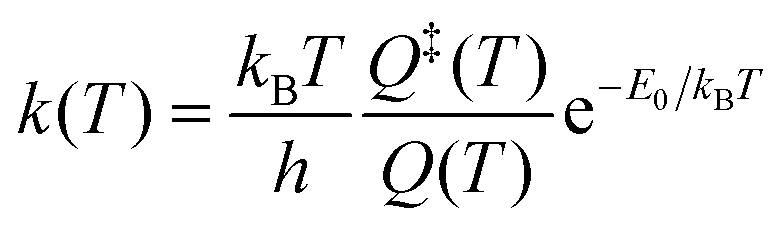
For this reason unimolecular fragmentation processes were largely studied both experimentally and theoretically.1 The central theory used to describe such process is the Rice–Ramsperger–Kassel–Marcus (RRKM) theory,13–15 which is typically formulated in the microcanonical ensemble1 and corresponds to the Transition State Theory (TST) in the canonical ensemble. Both theories provide a direct and simple relation between the rate constant and the threshold energy (E0) for the elementary reaction R → A + B (where R is the reactant and A and B the dissociation products):
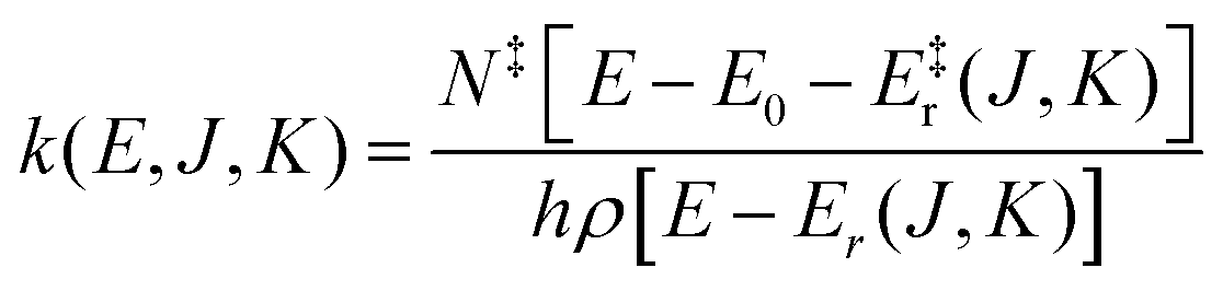 | (1) |
 | (2) |
Eqn (1) and (2) can be used to obtain the rate constants if the molecular information is available, or to obtain the threshold energy from rate constants at different energies or temperatures by a fitting procedure. In particular, the high-pressure limit TST unimolecular rate constant (eqn (2)) can be written and used as an Arrhenius equation:1
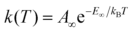 | (3) |
RRKM and TST are powerful theories which well describe kinetics of unimolecular dissociation but one needs to clearly identify the reaction pathway and locate the TS. While this is straightforward for simple processes, it may be very difficult for complex and flexible systems in which different pathways are present. In this context, molecular simulations, and notably direct dynamics, provide a useful tool to study the unimolecular fragmentation of such complex molecular systems. From such approach, it is possible not only to discover new reaction mechanisms and/or products, as when modeling collision- or surface-induced dissociation processes, but also to obtain the threshold and/or activation energies.18 In particular, Hase and co-workers have studied at different levels of theory relatively complex systems, showing how direct dynamics combined with unimolecular reaction theory is a powerful tool to get threshold or activation energies.19 Note that this is particularly useful for large systems, like e.g. poly-peptides, for which the localization of the corresponding TSs is highly problematic.20,21
One critical aspect when dealing with quantitative characterization of the reaction barrier from direct dynamics simulations is the zero-point energy (ZPE). In fact, when the ZPE is not the same for reactant and TS, the classical and quantum threshold energies do not correspond. Chemical dynamics simulations are often based on quasi-classical initial conditions followed by newtonian equations of motion numerical integration. In this way one can observe typical non-physical effects, like ZPE leakage22,23 or, as it is the case for simple unimolecular fragmentation, products with incorrect energy distribution. For the unimolecular fragmentation case, this is due to the fact that simulations can generate products with a vibrational energy which is less than the ZPE. This problem was recently discussed by Paul and Hase for the micro-canonical reactivity of a simple CH4 model.24 In this case, the unimolecular fragmentation consists in the H abstraction through a loose TS, such that one can consider just the difference between the ZPE of reactant (CH4) and of one product (CH3). These authors have proposed a relatively simple method in which, if a trajectory forms a product with an energy lower than the ZPE, the trajectory is sent back to the reactant basin. This approach can be seen as the unimolecular fragmentation version of one of the first methods proposed in the past to avoid ZPE leakage in direct dynamics simulations.22,23 While the rate constants obtained in this way qualitatively reproduce ZPE effects on the unimolecular rate constant, the resulting energy dependence did not show the expected RRKM behavior.25
Direct dynamics simulations in the canonical ensemble represent another possibility to obtain rate constants and then, from an Arrhenius fit, the activation energy. The resulting k(T) will be anharmonic and, if nuclear quantum effects are correctly accounted for, quantum. In the TST formulation, ZPE and anharmonicity effects are introduced in this case not only in the value of the activation energy but also in the quantum partition functions. A first approach was reported recently by Spezia and Dammak, where nuclear quantum effects were considered using the Quantum Thermal Bath (QTB).25 This approach is appealing because it requires a computational effort that is very similar to classical simulations. The QTB has also recently proved capable of capturing accurately the effects of ZPE in liquid water, both on equilibrium properties and on the vibrational spectrum.26 However, the quantum-classical activation energy differences reported in ref. 25 were overestimated, as further analyzed below.
Another very popular class of methods to account for nuclear quantum effects, that can be used in conjunction with direct dynamics simulations is that deriving from Path Integral theory.27–29 In particular, Ring Polymer Molecular Dynamics (RPMD)30 and Centroid Molecular Dynamics (CMD)31,32 are able to correctly predict reaction rate constants.33,34 While these methods have been used for isomerizations and bi-molecular simulations,33,35–41 detailed study of how they behave in the case of unimolecular fragmentation kinetics at different temperatures has not been reported in the literature so far.
Another class of methods is based on a thermal Wigner sampling of initial conditions, but they will likely suffer from two problems in this context: (i) they usually rely on the harmonic approximation for the sampling of the Wigner density, whereas fully anharmonic approaches rapidly become computationally heavy for large systems;42–44 (ii) since relatively long trajectories are needed for the fragmentation to occur, ZPE leakage from high to low frequencies might become problematic and bias the results. Other methods, like e.g. the Gaussian weighting in the quasi-classical trajectory method45 which is very powerful to study molecular scattering46,47 or dissociation of bimolecular complexes,48,49 are largely too expensive for medium-to-large molecular systems, require the knowledge of products and are generally used for well-defined state-to-state reactions. On the other hand, QTB and RPMD can be applied nowadays to relatively large molecules and sample a canonical ensemble. Since the aim of the present work is to assess how molecular simulation methods potentially useful to simulate large molecular systems in the canonical ensemble are able to take into account ZPE effects in fragmentation, all these other methods briefly discussed just above will not be considered here.
In the present work, we study the ability of direct dynamics simulations with QTB and RPMD approaches in quantitatively describing unimolecular fragmentation at different temperatures and in particular to capture the difference between classical and quantum rate constants and activation energies. To this end, we consider first a simple one-dimensional (1-D) Morse model, for which simulation results were compared with thermal rate constants from quantum theory50 using a sum-of-states approach. We then turn to the CH4 model, which is modified in order to represent different barrier heights and to explore different temperature ranges. This relatively simple molecular model is chosen in view of the solid experimental data for CH4 dissociation on a wide temperature range51–55 and because an analytical model has been developed56–58 which is known to be in agreement with experiments and kinetic theory.57,58 Simulation results can thus be compared with the available experimental and TST data. The simple analytical form of this model enables fast simulations and can be easily tuned to mimic molecular systems with lower dissociation energies, that can therefore be studied in direct dynamics simulations at lower temperatures. This study also illustrates the conditions for nuclear quantum effects to have a non-negligible impact on the rate constants.
2 Unimolecular rate constant
2.1 Quantum theory
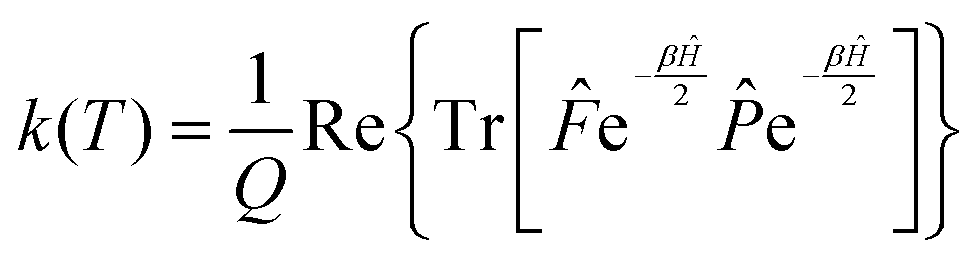
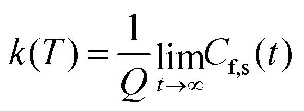
Following Miller and co-workers50,59 and using one-dimensional notations for simplicity, a formal expression of the Boltzmann rate constant k(T) can be written as: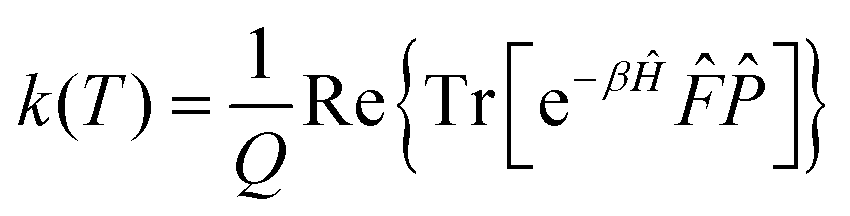 | (4) |
![[F with combining circumflex]](https://www.rsc.org/images/entities/i_char_0046_0302.gif) and
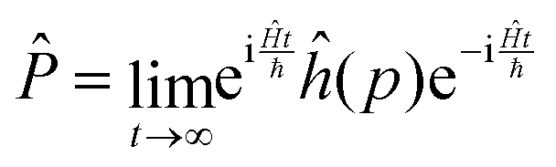
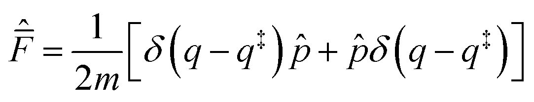
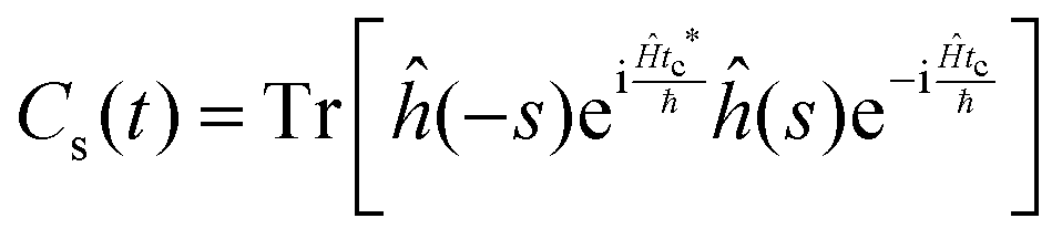
and ![[P with combining circumflex]](https://www.rsc.org/images/entities/i_char_0050_0302.gif) are the Hamiltonian, flux and projection operators, respectively. These two last operators are defined through the step function operator, ĥ, as follows:
are the Hamiltonian, flux and projection operators, respectively. These two last operators are defined through the step function operator, ĥ, as follows: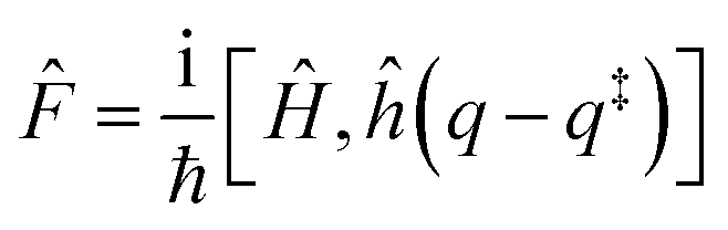 | (5) |
 | (6) |
Note that the step function operates on the position for the operator (more precisely on the distance to the transition state, q‡: s = q − q‡) and on the momentum, p, in the case of the operator . However, it can be shown that in the limit t → ∞, the step function operator ĥ(p) in can be replaced by ĥ(s).59
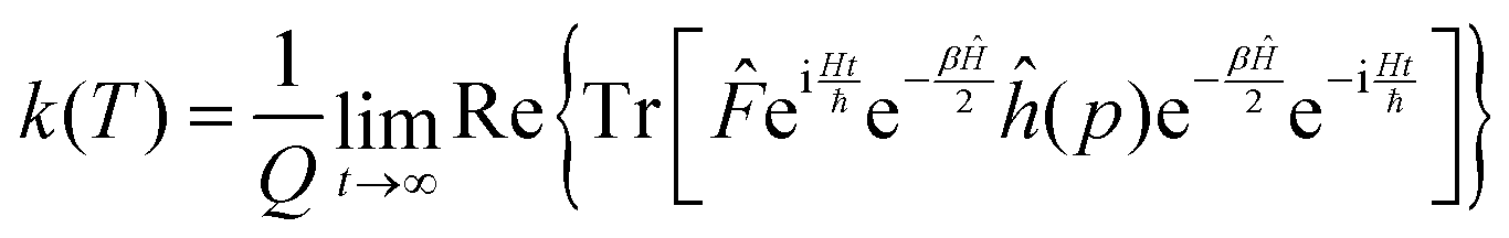
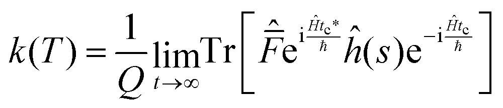
Since the operators and e−βĤ commute, the rate constant can be written in a more symmetric way:
 | (7) |
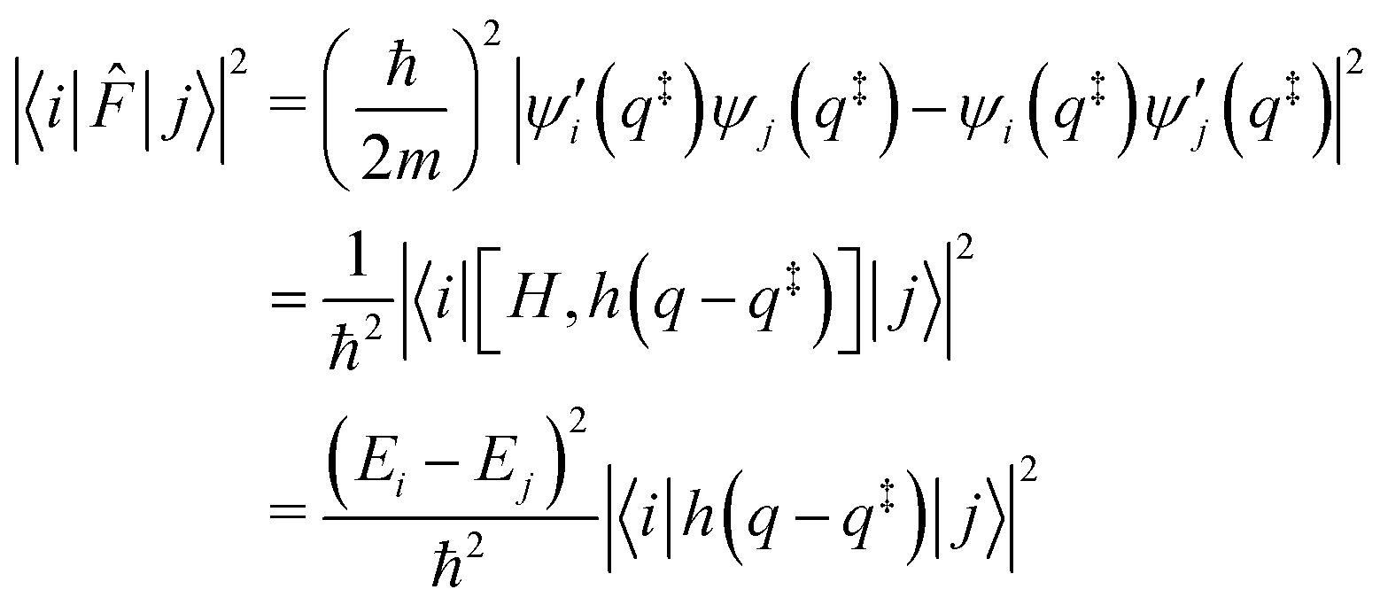
Using the explicit definition of the projection operator (see eqn (6)), we obtain:
 | (8) |
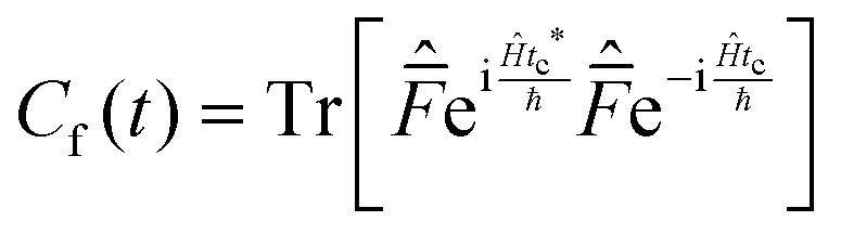
Introducing the complex time variable, tc = t − iħβ/2 and the symmetrized flux operator,
 | (9) |
 | (10) |
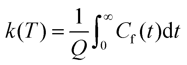
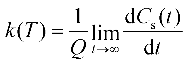
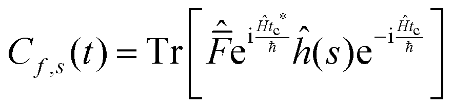
This final expression is particularly powerful since it can be connected with the quantum correlation functions, and notably:
 | (11) |
 | (12) |
 | (13) |
 | (14) |
 | (15) |
 | (16) |
This approach can be used directly for systems with few degrees of freedom by developing the expressions above on the eigenstate basis. We have used this Sum-of-State method (see Section 3.2 for details) to obtain the rate constant for the dissociation of a simple 1-D Morse model. Note that the rate constant as expressed in eqn (11)–(13) are formally the same if one employs the Kubo-transformed (or classical) correlation functions.33,60
2.2 Rate constants from direct dynamics simulations
From trajectory based simulations the rate constant can be obtained considering the flux through the transition state hypersurface and the correlation function(s) discussed previously (using classical correlation functions in the case of classical dynamics). When the temperature (or the energy) is high enough, the reactivity can be directly sampled and rate constants obtained. This was the case of a number of unimolecular fragmentation simulations studied by Hase and co-workers, ranging from small to large systems.18,19,61–63In unimolecular fragmentation, the time evolution of the reactants (N(t)) has the simple behaviour:
| N(t)/N(0) = e−kt | (17) |
Note that it was recently shown that the rate constant obtained in such a way converges more rapidly with the number of trajectories compared to those obtained by the flux approach.66
Each trajectory is considered to be converted to products when a given threshold distance is passed. Trajectories are then immediately stopped, so that they don’t allow for recrossing, as in the main assumption of transition state theory. For CH4 previous studies have set this threshold distance at 6 Å based on variational TST and we have used the same value.24,25 Notably, converged threshold values provide very similar rate constants21 and more importantly Arrhenius-like behaviours.66 Thus, once the rate constants for each unimolecular process are obtained at different temperatures, if an Arrhenius behavior holds (and it can be easily verified from the outcomes of the different simulations), then the activation energy can be obtained by simply fitting
| k(T) = Ae−βEa | (18) |
3 Simulations set-up
We now describe some details of the simulations performed, in terms of model potentials, determination of rate constants viaeqn (14), theoretical methods to include nuclear quantum effects and associated computational details.3.1 Model potentials
 | (19) |
| CH4 → CH3˙ + H˙ | (20) |
The potential energy function is represented by different terms:
| V = VMorse + Vang + Voop + Vnd | (21) |
To model different fragmentation regimes, we have considered the Morse term:
 | (22) |
• Potential A, which corresponds to the original model for CH4 fragmentation.
• Potential B, where the barrier was lowered down by about 50%.
• Potential C, where the barrier was lowered further down to 30 kcal mol−1, roughly corresponding to typical values of protonated systems.
The atomic masses are those of C and H (i.e. 12 and 1.008 amu, respectively) for the three potentials. Notably, we have modified two parameters of the Morse function for all the four bonds, Di and Bi, keeping the equilibrium geometry fixed (r0i = 1.09 Å). As a consequence the ZPEs of reactants and products are changed and thus also the “quantum” zero Kelvin barrier, DQ. The different sets of parameters are reported in Table 1, with the corresponding ZPEs and DQ, while in Fig. 1 we show the corresponding Morse functions.
| Potential | D i (≡ D(Cl)0) [kcal mol−1] | Bi [Å−1] | ZPER [kcal mol−1] | ZPEP [kcal mol−1] | D Q [kcal mol−1] |
|---|---|---|---|---|---|
| A | 109.460 | 1.944 | 29.18 | 19.38 | 99.66 |
| B | 50.000 | 2.500 | 26.76 | 16.74 | 39.98 |
| C | 30.000 | 3.000 | 25.63 | 16.54 | 20.91 |
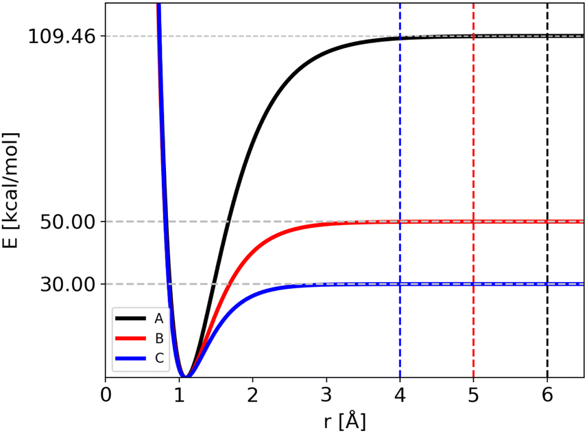 | ||
| Fig. 1 Morse functions used in the modified CH4 molecular system: potential A is in black, potential B in red and potential C in blue. Horizontal dotted lines show the corresponding D0 values, while vertical dashed lines show the position of the threshold distances used in trajectory simulations. | ||
3.2 Sum-of-states rate constants
The expressions (11)–(13) for the rate constant can be developed via a discrete basis set approach. We denote the eigenvalues {Ei} and the eigenfunctions {ψi(s)} corresponding to the eigenstates {|i〉} of the Hamiltonian: for a one-dimensional system, they are easily obtained by numerical diagonalization over an arbitrary set of basis functions. In this eigenstates representation, the flux correlation function in eqn (11) can be rewritten as:where we introduced the resolution of identity:
 . The rate constant thus becomes:
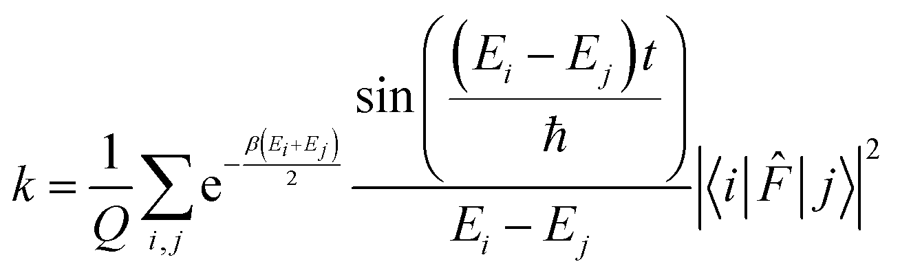 | (23) |
Finally, the flux matrix element is related to the wave functions by two different, equivalent, expressions:
Note that a classical counterpart to this rate expression can easily be obtained by noting that, for the one-dimensional Morse function, the long-time limit of the flux-side correlation function is given by:
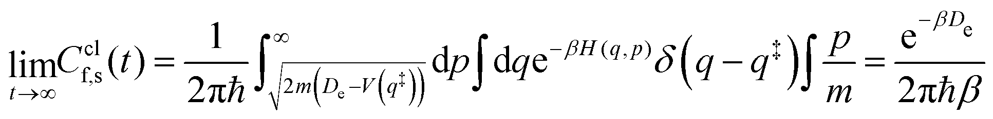 | (24) |
3.3 Ring-polymer MD
Ring Polymer Molecular Dynamics (RPMD)30 is a particular formulation of Path Integral Molecular Dynamics in which the system evolves on the effective Hamiltonian: | (25) |
 | (26) |
 | (27) |
In the RPMD formulation, we define the bead-average of a given property a(t) (position, momentum, but also distance etc…) as:
 | (28) |
 | (29) |
As discussed previously, a threshold distance is used to decide if the reaction has occurred: in the RPMD formalism this should be obtained from the bead average of distances between atoms l and k:
 | (30) |
In order to perform constant temperature simulations, we use the T-RPMD scheme with an additional mild thermostat on the centroid (with a friction coefficient denoted γ), following the integration algorithm proposed by Ceriotti et al.69 which is reported in details in the ESI.†
The number of beads was set to reach convergence of the potential and kinetic energies for each temperature. Classical simulations correspond to P = 1.
3.4 Quantum thermal bath
Another possibility to account for NQE in trajectory-based simulations is by using the quantum thermal bath (QTB).70 This method is based on Langevin equations of motion: | (31) |
 | (32) |
 | (33) |
In classical Langevin simulations, a white noise IRi(ω) = 2miγkBT is used instead of eqn (33), which leads to the equipartition of energy. In the QTB, on the other hand, the average (vibrational) energy includes a ZPE contribution and in the harmonic approximation, it depends on the ![[small script l]](https://www.rsc.org/images/entities/char_e146.gif) vibrational frequencies of the system (ωi):
vibrational frequencies of the system (ωi):
 | (34) |
QTB simulations have almost the same computational cost as classical simulations, since the only additional calculation is the generation of the colored noise. Here we have generated it using the original algorithm proposed by Dammak and co-workers70 and the equations of motions were solved using the modified velocity-Verlet algorithm. Note that in the QTB each atom is represented by a unique position vector and thus each quantity is obtained as from classical dynamics (and notably the distance which is used to identify when a system reacts). The QTB approach is originally designed to account for the consequences of ZPE on the thermal equilibrium distribution of the system and on the resulting (time-independent) properties. However, it was also shown recently to be able to capture subtle quantum effects on the vibrational dynamics of molecular systems,26,72 so that one can wonder if it could also be used in a direct dynamics set up. A recent review of the QTB method and its applications can be found in ref. 73.
3.5 Computational details
| T (K) | P | |
|---|---|---|
| 1D Morse | 800 | 32 |
| 900 | 16 | |
| 1000 | 8 | |
| 1100 | 8 | |
| 1200 | 8 | |
| Potential A | 3000 | 8 |
| 3500 | 8 | |
| 4000 | 8 | |
| 4500 | 8 | |
| 5000 | 8 | |
| Potential B | 1350 | 16 |
| 1500 | 8 | |
| 1700 | 8 | |
| 2000 | 4 | |
| 2500 | 4 | |
| Potential C | 800 | 16 |
| 1000 | 16 | |
| 1200 | 8 | |
| 1500 | 8 |
LMD simulations were performed as previously but setting P = 1 for each temperature, while the QTB simulations were performed considering the same parameters as in LMD simulations.
The trajectories were carried out for different ranges of temperature, listed in Table 2, to allow the fragmentation of the reactant. If the distance of one bond reaches the cut-off value, the trajectory is stopped and the lifetime collected. The cut-off value used in ref. 24 for the Potential A (6 Å) corresponds to a plateau in the Morse potential energy function: the cut-off values for Potentials B and C (5 and 4 Å, respectively) where reduced since the dissociation energy is reached at shorter distances (see Fig. 1). The maximum simulation time was set to 5 ns, with a time-step of 0.1 fs. As before, the number of beads used in RPMD simulations was chosen in order to converge the average energy: in Table 2 we list the number of beads used for each potential as a function of temperature.
The friction parameter γ was chosen in order to yield a fast enough temperature equilibration, as illustrated by the temperature autocorrelation function reported in Fig. S1 of the ESI.† Notably, γ = 0.01 fs−1 provides an efficient thermostat for this system, whereas smaller values would result in a too slow equilibration (here the equilibration should be faster than the typical reaction time) and too large values can affect the dynamical results (in particular in the overdamped regime).
To obtain rate constants and the associated uncertainties from trajectory simulations, we implemented the bootstrap algorithm.76 This statistical method randomly re-samples a single data-set, to create multiple data-sets and obtain the mean and the standard deviation from a Gaussian distribution. In the present case the data set consists in the set of reaction times for each individual trajectory and for each re-sampling, we computed the associated rate constant from single exponential fitting.
4 Rate constants and activation energies
4.1 1-D model potential
For the 1-D Morse potential we calculated the quantum rate constants using the Sum-of-States (SoS) approach, eqn (23), detailed previously. Classical rate constants can also be directly obtained. These results are used as reference calculation to evaluate the performances of LMD, RPMD and QTB simulations.In the SoS approach the rate constant is obtained from the t → ∞ limit of the function Cf,s(t)/Q. The time dependence of this function is shown in Fig. 2 for the 1-D Morse model at two temperatures, 800 and 1500 K. As discussed in details by Miller in the past,50,59 for such low-dimensional system, the function actually goes to zero in the long-time limit, but the value of the rate k can still be obtained by considering the maximum (plateau) of the function in an intermediary time range. In the same plots we also report the corresponding classical rate constant as an horizontal black line.
 | ||
| Fig. 2 Quantum (red) and classical (black) rate constants obtained with the SoS method for the 1-D Morse at two different temperatures: 800 K (left) and 1500 K (right). | ||
Rate constants obtained in an extended temperature range (700–1200 K) are shown in Fig. 3 while all the values are listed in Tables S1 and S2 of the ESI† (where we also list the corresponding lifetimes). It is important to notice that the rate constants show an Arrhenius-like behavior, and thus we were able to fit them and obtain activation energies in both classical and quantum regimes. Values are reported in Table 3 together with the difference between classical and quantum activation energies. These results can now be used as reference to evaluate values obtained from trajectory simulations.
 | ||
| Fig. 3 Quantum and classical rate constants as a function of temperature for the 1-D Morse. In full lines we report values obtained from sum-of-state approach (both classical and quantum), while results from trajectory simulations (γ = 0.01 fs−1) are reported as dots: LMD (black), RPMD (red) and QTB (green). | ||
| Method | E a | ln(A) | ΔECl–Q |
|---|---|---|---|
| Classical reference | 9.49 | 3.34 | — |
| Quantum (SoS) | 8.74 | 3.13 | 0.75 |
| LMD (γ = 0.01) | 8.60 ± 0.09 | 2.31 ± 0.05 | — |
| RPMD (γ = 0.01) | 7.8 ± 0.1 | 2.12 ± 0.08 | 0.8 ± 0.1 |
| QTB (γ = 0.01) | 1.3 ± 0.2 | 0.6 ± 0.1 | 7.3 ± 0.2 |
| LMD (γ = 0.045) | 9.70 ± 0.03 | 3.09 ± 0.01 | — |
| RPMD (γ = 0.045) | 8.85 ± 0.02 | 2.83 ± 0.01 | 0.85 ± 0.04 |
| QTB (γ = 0.045) | 1.74 ± 0.08 | 1.08 ± 0.05 | 7.96 ± 0.08 |
| LMD (γ = 0.3) | 9.9 ± 0.2 | 2.1 ± 0.1 | — |
| RPMD (γ = 0.3) | 9.21 ± 0.1 | 1.91 ± 0.07 | 0.7 ± 0.2 |
| QTB (γ = 0.3) | 5.8 ± 0.4 | 1.1 ± 0.2 | 4.1 ± 0.4 |
| Harmonic classic | 8.11 | — | — |
| Harmonic Quantum | 7.33 | — | 0.78 |
Trajectory simulations (LMD, RPMD and QTB) were performed on the same temperature range and for all of them we observed a single exponential decay of the reactant populations, such that rate constants could be extracted directly by fitting eqn (17) with the bootstrap method to assign the associated uncertainties. An example is shown in Fig. 4, corresponding to simulations at 800 K and γ = 0.01 fs−1 done with LMD, RPMD and QTB methods. Similar single exponential decays are obtained at other temperatures and γ values. As we can already see, while LMD and RPMD provide quite similar decays, the QTB reaction rate is much faster. We discuss this aspect further in the following.
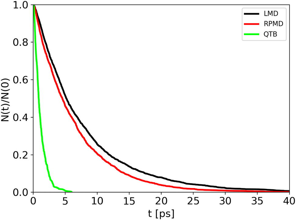 | ||
| Fig. 4 Population decay for 1-D Morse simulations at 800 K as obtained from LMD, RPMD and QTB trajectories. | ||
Rate constants obtained from trajectories as a function of temperature are shown in Fig. 3 for γ = 0.01 fs−1 (and all the values are reported in the same Tables S1 and S2 of ESI,† with the corresponding lifetimes). We can notice that LMD and RPMD simulations show a clear Arrhenius-like behavior, with a slope which is similar to that obtained via the SoS method, and rate constant values of the same order of magnitude as the reference. On the other hand, in QTB simulations, the rate constants are much higher and they show only weak variations with temperature.
The corresponding activation energies and pre-exponential factors are reported in Table 3 where they can be compared with SoS values. Remarkably, activation energies obtained from LMD and RPMD simulations are very similar to those obtained from the SoS and classical reference approaches.
In simulations discussed previously, we have used a friction parameter γ of 0.01 fs−1. We also performed simulations with two additional γ values (0.045 and 0.3 fs−1) to investigate if there is an impact on kinetics, activation energy and, more importantly, quantum-classical difference. Note that γ = 0.3 fs−1 corresponds to an overdamped regime (γ ∼ ω with ω the typical angular frequency of the Morse potential). The lifetimes (and rate constants) vary with γ, but this variation is very small as shown by the Arrhenius plots (Fig. S2 and S3 in the ESI†).
From the rate constants as a function of temperature with different γ values, we performed Arrhenius fits to obtain activation energies which display almost no dependence on γ, as shown in Table 3.
If we now move to the difference between the classical and quantum activation energies, we notice that RPMD simulations are in very good agreement with SoS values, while QTB largely overestimates it. Furthermore, the effect of γ on this quantity almost vanishes, in particular for RPMD simulations.
Before moving to the study of a more complex molecular system, we consider here also the simple harmonic approximation (both classical and quantum) to estimate the barrier. Notably, we can approximate the barrier for a simple dissociation as the average energy difference between reactants and products. In the case of a simple 1-D Morse model, we have:
| Ei(T) = EiPOT + EiTR(T) + EiVIB(T) | (35) |
| ΔE(T) = ΔEPOT + ΔETR(T) − EreactVIB(T) | (36) |
The energy difference between classical and quantum approach is thus simply reduced to:
| ΔECl–Q(T) = EClVIB(T) − EQVIB(T) | (37) |
Results are reported in the same Table 3. Although the average energy difference tends to slightly underestimate the activation energy in absolute value, the quantum-classical difference obtained with this method is very similar to that derived from the SoS approach (and to what is obtained comparing LMD with RPMD simulations). This will be very important for the study of a more complex molecular system for which the SoS approach is not feasible, and the simple Harmonic approximation can provide a good reference to compare trajectory simulations with.
4.2 CH4-based potentials
We now discuss the rate constants obtained for the unimolecular fragmentation of the CH4 model (potential A) as a function of temperature and how this behavior is modified by decreasing the barrier (potentials B and C).From trajectory simulations we obtained the population decay as a function of time which shows, also in this case, a single exponential behaviour. The single-exponential behaviour was found for each temperature, potential and method (see a prototypical example reported in Fig. 5). Thus, we were able to extract lifetimes and unimolecular rate constants.
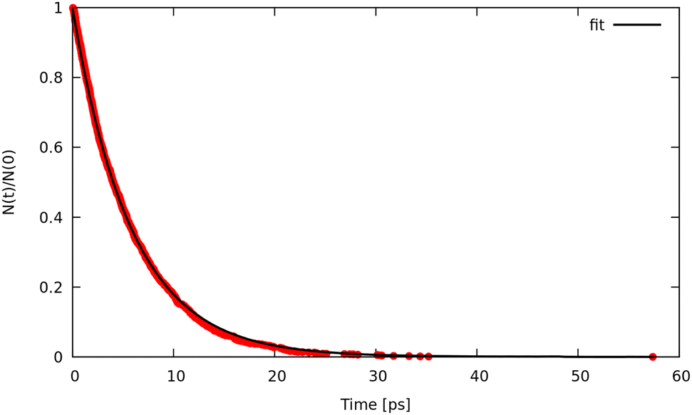 | ||
| Fig. 5 Population decay obtained from RPMD simulations with γ = 0.01 fs−1, P = 8 and T = 4500 K using Potential C. Red dots are the simulation data, black solid line corresponds to a single-exponential fit. | ||
LMD, RPMD and QTB rate constants as a function of temperature are shown in Fig. 6 for the three potentials, while the full set of values (both lifetimes and rate constants) is reported in Tables S3–S8 of the ESI.† Experimental data are available only for potential A, corresponding to CH4 fragmentation. The best sets of values to be compared with unimolecular rate constants from simulations (where the colliding gas is not explicitly simulated such that they have inverse time dimensions) are those reported by Cobos and Troe51,52 which also provide an analytical function to express k(T), originally in the 300–3000 K temperature range later extended up to 5000 K. Simulation results agree well with such experimental data as shown in Fig. S4 of the ESI.†
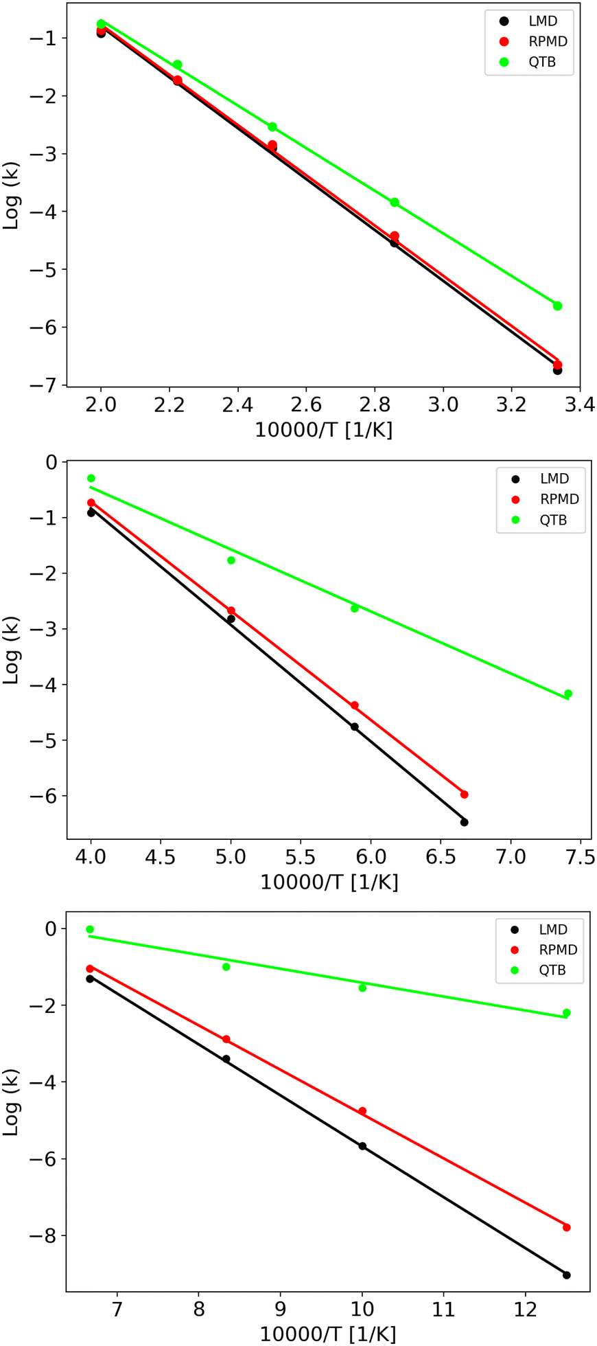 | ||
| Fig. 6 Arrhenius plots obtained from LMD, RPMD and QTB simulations for A, B and C potentials (from top to bottom). Circles are data obtained from the simulations while lines represent the fit results. | ||
The capacity of the RPMD and the QTB to correctly capture nuclear quantum effects can be first assessed by comparing the ratio between the quantum and classical rate constants (kq and kcl, respectively) with that obtained from transition state theory (TST), which typically holds for CH4 fragmentation.24,77,78 Results are summarized in Table 4 where to evaluate the partition function ratio for TST we employed the rigid-rotor harmonic approximation both classical and quantum.1 The nuclear quantum effects are limited for Potential A, while they increase for potentials B and C, as expected since we were able to simulate lower temperatures. Notably, the kq/kcl values obtained from TST are very similar to the RPMD/LMD ratios, while the QTB largely overestimates the rate constants, in agreement with what was found for the simple 1-D Morse model. The slight differences between the TST and RPMD/LMD results can be ascribed to anharmonicity effects that are present in the simulations while not accounted for by the TST harmonic approximation for the partition function. This effect is more marked for potentials B and C where the barrier is lower and therefore anharmonicity is likely more important. Note that the CH4 experimental data (see aforementioned Fig. S4 in the ESI†) are in better agreement with RPMD (and quantum TST) values than with the QTB ones.
| T[K] | k TST,q/kTST,cl | k RPMD/kLMD | k QTB/kLMD | |
|---|---|---|---|---|
| Pot. A | ||||
| 3000 | 1.17 | 1.09 | 3.04 | |
| 3500 | 1.12 | 1.12 | 2.01 | |
| 4000 | 1.09 | 1.06 | 1.44 | |
| 4500 | 1.07 | 1.02 | 1.33 | |
| 5000 | 1.06 | 1.04 | 1.17 | |
| Pot. B | ||||
| 1350 | 1.86 | 1.71 | 54.3 | |
| 1700 | 1.49 | 1.48 | 5.68 | |
| 2000 | 1.34 | 1.16 | 2.85 | |
| 2500 | 1.21 | 1.19 | 1.88 | |
| Pot. C | ||||
| 800 | 4.49 | 3.53 | 896 | |
| 1000 | 2.72 | 2.47 | 60.90 | |
| 1200 | 2.04 | 1.69 | 11.00 | |
| 1500 | 1.59 | 1.29 | 3.64 | |
| 1800 | 1.39 | 1.36 | 2.03 | |
As clearly shown in Fig. 6, we obtain Arrhenius-like behaviors in all simulations such that we were able to fit them and derive activation energies. They are reported in Table 5 together with the corresponding quantum-classical differences. We should notice that for all the potentials, the RPMD activation energies are much closer to the LMD ones than what is obtained from QTB simulations: for the Potential A, which has a high barrier and for which, therefore, the simulations were performed at relatively high temperatures, this difference is negligible, comparable to the uncertainty, while for the QTB it is about 15 kcal mol−1 which is similar to the quantum-classical difference of the model at 0 K (namely the difference in ZPE between reactant and products, that is around 10 kcal mol−1). Moving to potentials B and C, we observe a statistically significant quantum-classical difference from RPMD (3.1 and 3.3 kcal mol−1, respectively) and, as before, larger values from the QTB. Note that the 0 K quantum-classical difference does not change much moving to potentials B and C, while QTB provides even larger values of activation energy quantum-classical differences.
![[T with combining macron]](https://www.rsc.org/images/entities/i_char_0054_0304.gif) )Cl) and quantum (ΔE()Q)
)Cl) and quantum (ΔE()Q)
| Pot. A | Pot. B | Pot. C | ||||
|---|---|---|---|---|---|---|
| Method | E a | ΔE | E a | ΔE | E a | ΔE |
| LMD | 88 ± 2 | — | 43.9 ± 0.2 | — | 26.2 ± 0.4 | — |
| RPMD | 87 ± 2 | 1 ± 3 | 40.8 ± 0.9 | 3.1 ± 0.9 | 22.9 ± 0.4 | 3.3 ± 0.6 |
| QTB | 73.3 ± 0.9 | 15 ± 2 | 22 ± 1 | 22 ± 1 | 7.2 ± 1.0 | 19 ± 1 |
| ΔE()Cl |
97.52 | — | 45.11 | — | 26.24 | — |
| ΔE()Q |
95.99 | 1.52 | 41.82 | 3.29 | 22.87 | 3.37 |
As previously done for the 1-D Morse model, it is possible to use the simple harmonic approximation approach to evaluate how the reaction barrier is temperature dependent and compare with simulation results. This simple approach was shown to provide reasonable results compared with the SoS method for the 1-D Morse model and thus it can also be used to evaluate the accuracy of the RPMD and QTB results for the molecular model case.
In particular, we can estimate the temperature dependent average energy difference (both classical and quantum and their difference) from
 | (38) |
 | (39) |
| ΔΔECl–Q(T) = ΔΔECl–QVIB(T) + ΔΔECl–QROT(T) | (40) |
In Table 5 we report the temperature averaged barrier values, that are slightly higher than the activation energy obtained from the Arrhenius plots, in particular for the potential A for which the simulations were performed at relatively high temperatures. However, the quantum-classical energy differences are in excellent agreement with the LMD-RPMD differences for the three potentials. In particular, while for potential A (in the temperature range considered) there is almost no difference between classical and quantum vibrations, quantum effects are larger for potentials B and C: even if the difference remains small, it is significant compared to the statistical uncertainty in the simulation results.
In Fig. 7 we show the products-reactant energy difference as a function of temperature as obtained for potentials A and C using both classical and quantum energies (results for potential B are analogous and not shown for the sake of clarity). The plots also illustrates the limit of the “low” temperature region for each potential. It corresponds to temperatures below the ZPE (shown as vertical dotted lines), which is the point from which the classical and quantum energy curves begin to diverge significantly. We should note that for Potential A simulations were done at temperatures higher than the ZPE, in an almost classical regime (lower temperatures were not accessible due to computational limitations in trajectories time-length), while for Potential C (and B) it was possible to run trajectories at temperatures that are lower than the ZPE and so in a region where nuclear quantum effects are detectable. As a consequence, for Potential A the quantum-classical energy differences are almost irrelevant, while for Potential C the difference becomes noticeable. RPMD simulations are able to catch this effect accurately.
 | ||
| Fig. 7 Energy differences between products and reactant as a function of temperature in the harmonic approximation as obtained from Potentials A (upper panel) and C (lower panel). Full lines are classical values, while dashed lines are quantum ones. Vertical lines show the ZPE in K. | ||
It is well known that the absolute value of the activation energy is often underestimated from Arrhenius fits,67,79 but the quantum-classical difference, which mainly reflects the ZPE energy difference between reactants and products absent in classical dynamics, are well reproduced by the comparison between RPMD and LMD simulations.
Clearly, QTB rate constants and activation energies are much higher than that obtained from the other methods. Even if the harmonic approximation is rather crude, the present results together with that obtained from the 1-D Morse model, suggest that QTB overestimates unimolecular fragmentation rates in this case, while RPMD gives results in very good agreement with the quantum theory.
4.3 Distance distributions
Unimolecular fragmentation is obviously related to how the bond distance evolves from equilibrium to the threshold distance. Chemical reactivity in the canonical ensemble is related to energy fluctuations,80 and thus to distance fluctuations. As a consequence, even small differences in the distance distribution can cause large differences in reaction dynamics. In particular the tail of the distribution plays a crucial role. We have thus analyzed the distance distributions as obtained in different simulations (and theory for the simple 1-D Morse) at some relevant temperatures.We first consider the 1-D Morse model at 1000 K: in Fig. 8 we report the classical and quantum analytical distributions and how simulations compare with them. In the case of RPMD simulations we plot two quantities: the distribution of the atomic distance for each bead (marked in the figure as “RPMD-Beads”) as well as the distribution of the centroid of the distance, i.e. its average over all beads as in eqn (30) (marked in the figure as “RPMD-Centroid”).
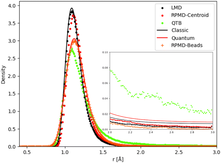 | ||
| Fig. 8 Distance distribution (as probability density) for 1-D Morse model at 1000 K. In the inset we show a zoom of the distribution tail. | ||
As one should expect by construction, the LMD distance distribution essentially coincides with the classical theoretical distribution, while the RPMD-Beads curve is almost superimposed with the quantum reference. The quantum distribution is significantly broader than the classical one, due to the non-negligible ZPE effects, even at this relatively high temperature. The maximum of the quantum peak is also slightly displaced with respect to its classical counterpart. The QTB distribution is broadened in a similar way as the quantum reference, showing that the colored noise thermostat provides an approximation to ZPE effects. However, the peak maximum is slightly displaced with respect to the quantum reference (it is more in line with the maximum of the classical distribution), and more importantly, the long-distance tail of the distribution is markedly longer in the QTB simulations. These slight inaccuracies of the QTB approximation have been discussed in the literature in the non-reactive case (see for example ref. 73), where they usually have only minor consequences. However, the shape of the distribution tail can have a much larger impact on the unimolecular fragmentation rate and partly explain its overestimation by the QTB. The RPMD-Centroid curve is also instructive: the distribution of the centroid distance is very similar to the classical distribution, with only a slight shift of its maximum towards longer distances as for the quantum distribution. This behavior is even amplified at lower temperatures, where the classical and RPMD-Centroid distributions become sharper and sharper, while the RPMD-Beads curve remains essentially unchanged and fixed by the ZPE of the system. Therefore in the low-temperature regime, even if the beads are still allowed to explore a relatively broad range of distances, the bead-averaged distance remains close to the equilibrium distance, indicating that the broadening of the distribution is caused by the eventual excursion of individual beads, while the core of the ring-polymer remains trapped in the vicinity of the equilibrium position. This mechanism effectively suppresses the fragmentation process at low temperatures, since the latter implies that the whole polymer (and hence also its centroid) detaches from the equilibrium position. There is no such effect in QTB simulations, where the ZPE is introduced as an effective temperature that depends on the characteristic frequency of the system. As a consequence, the QTB fragmentation rate tends to a non-zero limit for T → 0, in contradiction with what is expected from the SoS approach (and from RPMD).
The distributions obtained for the C–H distance in the CH4 model potential show a very similar behaviour. We present in Fig. 9 as an example the results obtained for Potential C at 1000 K (in this case we run simulations with a larger distance cut-off of 5 Å, to enhance the statistics on the tail of the distribution). As in the 1-D Morse model, the centroid distribution of the distance is much sharper than that of the beads and closer to the classical results. The narrow centroid distribution explains why the RPMD reaction rate is significantly lower at this temperature than the QTB one, even though the QTB provides a very good approximation to the RPMD-Beads distribution (with only a slight shift of the peak maximum, as noted previously). Indeed, in RPMD simulations, even if individual beads can undergo momentary increase of the C–H bond length, the harmonic spring forces of the ring-polymer then tend to attract it back towards the equilibrium distance (where the centroid tends to remains localized), whereas no such mechanism exist in the case of the QTB.
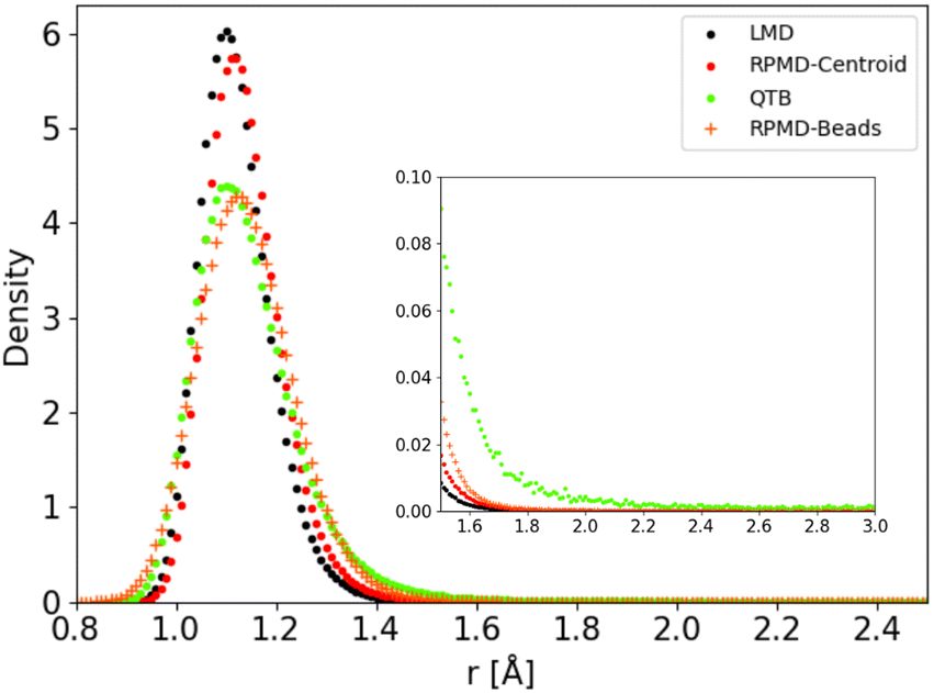 | ||
| Fig. 9 C–H distance distribution as obtained from trajectory simulations using Potential C at 1000 K. | ||
5 Conclusions
In the present work, we have investigated how the unimolecular reaction is modified when passing from a classical to a quantum description of the nuclear motion. In particular, we have investigated how reaction rates and activation energies are affected and how direct dynamics simulations based on an ensemble of trajectories are able to reproduce this behavior. We have compared simulation results with quantum rate constant theory for a simple 1-D Morse model and then studied a more complex molecular model tuning the barrier height.Results show that Ring Polymer Molecular Dynamics (RPMD) is able to correctly catch the unimolecular kinetics, and how it is impacted by nuclear quantum effects. This confirms previous studies by Manolopoulos and co-workers on different reactions such as isomerizations and bi-molecular reactions.33,35,36 In particular in the low temperature regime, although the beads probability distribution (which represents the physical quantum distribution) is strongly broadened by the zero-point motion, the centroid distribution remains localized in a similar way as for a classical system. Since the fragmentation process requires the whole polymer to go through the barrier, the localization of the centroid effectively reduces the reaction rate at low temperatures, in agreement with the quantum theory. The Quantum Thermal Bath (QTB) on the other hand, largely overestimates the reaction rates, in particular for low barriers, or when the temperature becomes lower than the zero-point energy (ZPE). The QTB approximates ZPE as an elevated effective temperature via a colored-noise thermostat. Although this approach proves accurate to describe ZPE effects on the equilibrium distribution, it cannot be used to compute fragmentation rates in a direct dynamics set-up.
The temperature dependence of the quantum/classical rate constant ratio shows that nuclear quantum effects can be relevant even at relatively high temperatures. In fact, we observed that, even at 800 and 1000 K, the quantum rate constants are about 4 and 2.5 times faster than the corresponding classical values, respectively. The temperature range for which the NQEs are relevant is related to the ZPE of the corresponding breaking bond.
The present study suggests that RPMD methods can be used as trajectory based method to investigate unimolecular reactions of complex systems. This approach can be a powerful alternative to transition state theory to study fragmentation of large molecules, having many fragmentation pathways and for which the determination of all the corresponding transition states may be difficult,19 while clearly it will not supersede TST for systems in which it can be applied. For example, the fragmentation of complex peptides was recently studied with newtonian reaction dynamics not only to study qualitatively the fragmentation pathways but also to evaluate quantitatively the activation energies.18,20,21 Future studies could be now done using RPMD to investigate the role of NQEs on both aspects. Such direct dynamics approach is able to provide anharmonic rate constants in which nuclear quantum effects are taken into account. In terms of transition state theory this corresponds to (i) taking into account the ZPE effect on the barrier height and (ii) considering the quantum partition functions without any specific approximation (like the typical harmonic approximation): the effect is directly obtained on the resulting rate constant without the need of any specific correction. While all these aspects can be considered using transition state theory (eqn (2)), one has to determine the reaction pathways which can be not obvious for large and flexible molecules: RPMD provides it directly from an ensemble of trajectories in a relatively simple way.
Clearly, one critical aspect to apply RPMD to large systems is the computational cost, which is roughly multiplied by the number of beads. However, the recent and future advent of fast and reliable reactive potentials based, for example, on machine learning techniques, will make possible to study fragmentation dynamics on much larger systems and the inclusion of nuclear quantum effects will also be computationally possible. The very good agreement between RPMD and TST on fragmentation reactions gives confidence of using RPMD when using TST may have practical problems, as for large and flexible molecules. Finally, the present work suggests to use RPMD approach when studying “low” temperatures, when “low” does not only mean few Kelvin degrees, but more in general temperatures in which zero-point energy effects are relevant.
Author contributions
F. Angiolari was responsible for data curation and visualisation of results. F. Angiolari and S. Huppert were responsible of software coding. R. Spezia and S. Huppert equally contributed to conceptualisation and supervision of the entire work. R. Spezia wrote the initial draft. All the authors contributed together in reviewing/editing of the manuscript.Conflicts of interest
There are no conflicts to declare.Acknowledgements
The authors thank Dr Sara Bonella, Dr Philippe Depondt and Dr Fabio Finocchi for fruitful discussions.Notes and references
- T. Baer and W. L. Hase, Unimolecular reaction dynamics: theory and experiments, Oxford University Press, New York, 1996 Search PubMed.
- E. de Hoffmann and V. Stroobant, Mass Spectrometry. Principles and Applications, Wiley, Chichester, West Sussex, England, 2007 Search PubMed.
- J. H. Gross, Mass Spectrometry. A Textbook, Springer, 2004 Search PubMed.
- I. A. Papayannopoulos, Mass Spectrom. Rev., 1995, 14, 49–73 CrossRef CAS.
- J. Zaia, Mass Spectrom. Rev., 2004, 23, 161–227 CrossRef CAS PubMed.
- B. Paizs and S. Suhai, Mass Spectrom. Rev., 2005, 24, 508–548 CrossRef CAS PubMed.
- J. Laskin and J. H. Futrell, Mass Spectrom. Rev., 2003, 22, 158–181 CrossRef CAS PubMed.
- M. T. Rodgers and P. B. Armentrout, Mass Spectrom. Rev., 2000, 19, 215–247 CrossRef CAS.
- P. B. Armentrout, Annu. Rev. Phys. Chem., 2001, 52, 423–461 CrossRef CAS PubMed.
- P. B. Armentrout, Int. J. Mass Spectrom., 2003, 227, 289–302 CrossRef CAS.
- A. Merkel, Z. Havlas and R. Zahradnik, J. Am. Chem. Soc., 2003, 110, 8355–8359 CrossRef.
- P. Manikandan, J. Zhang and W. L. Hase, J. Phys. Chem. A, 2012, 116, 3061–3080 CrossRef CAS.
- O. K. Rice and H. C. Ramsperger, J. Am. Chem. Soc., 1927, 49, 1617–1629 CrossRef CAS.
- L. S. Kassel, J. Phys. Chem., 1928, 32, 225–242 CrossRef CAS.
- R. A. Marcus, J. Chem. Phys., 1952, 20, 359–364 CrossRef CAS.
- J. Troe and V. G. Ushakov, J. Chem. Phys., 2012, 136, 214309 CrossRef CAS PubMed.
- L. Zhu and W. Hase, Chem. Phys. Lett., 1990, 175, 117–124 CrossRef CAS.
- A. Martin-Somer, V. Macaluso, G. L. Barnes, L. Yang, S. Pratihar, K. Song, W. L. Hase and R. Spezia, J. Am. Soc. Mass Spectrom., 2020, 31, 2–24 CrossRef CAS PubMed.
- L. Yang, R. Sun and W. L. Hase, J. Chem. Theory Comput., 2011, 7, 3478–3483 CrossRef CAS PubMed.
- Z. Homayoon, S. Pratihar, E. Dratz, R. Snider, R. Spezia, G. Barnes, V. Macaluso, A. Martin-Somer and W. L. Hase, J. Phys. Chem. A, 2016, 120, 8211–8227 CrossRef CAS PubMed.
- R. Spezia, A. Martin-Somer, V. Macaluso, Z. Homayoon, S. Pratihar and W. L. Hase, Faraday Discuss., 2016, 195, 599–618 RSC.
- J. M. Bowman, B. Gazdy and Q. Sun, J. Chem. Phys., 1989, 91, 2859–2862 CrossRef CAS.
- W. H. Miller, W. L. Hase and C. L. Darling, J. Chem. Phys., 1989, 91, 2863 CrossRef CAS.
- A. Paul and W. L. Hase, J. Phys. Chem. A, 2016, 120, 372–378 CrossRef CAS PubMed.
- R. Spezia and H. Dammak, J. Phys. Chem. A, 2019, 123, 8542–8551 CrossRef CAS PubMed.
- N. Mauger, T. Plé, L. Lagardère, S. Bonella, E. Mangaud, J.-P. Piquemal and S. Huppert, J. Phys. Chem. Lett., 2021, 12, 8285–8291 CrossRef CAS PubMed.
- R. P. Feynman and A. R. Hibbs, Quantum mechanics and path integrals, McGraw-Hill, New York, 1965 Search PubMed.
- B. J. Berne and D. Thirumalai, Annu. Rev. Phys. Chem., 1986, 37, 401–424 CrossRef CAS.
- D. Marx and M. Parrinello, J. Chem. Phys., 1996, 104, 4077 CrossRef CAS.
- I. R. Craig and D. E. Manolopoulos, J. Chem. Phys., 2004, 121, 3368 CrossRef CAS PubMed.
- J. Cao and G. A. Voth, J. Chem. Phys., 1994, 100, 5093 CrossRef CAS.
- J. Cao and G. A. Voth, J. Chem. Phys., 1994, 100, 5106–5117 CrossRef CAS.
- I. R. Craig and D. E. Manolopoulos, J. Chem. Phys., 2005, 123, 034102 CrossRef PubMed.
- E. Geva, Q. Shi and G. A. Voth, J. Chem. Phys., 2001, 115, 9209–9222 CrossRef CAS.
- R. Collepardo-Guevara, Y. V. Suleimanov and D. E. Manolopoulos, J. Chem. Phys., 2009, 130, 174713 CrossRef PubMed.
- R. Perez de Tudela, F. J. Aoiz, Y. V. Suleimanov and D. E. Manolopoulos, J. Phys. Chem. Lett., 2012, 3, 493–497 CrossRef CAS PubMed.
- Y. Li, Y. V. Suleimanov, M. Yang, W. H. Green and H. Guo, J. Phys. Chem. Lett., 2013, 4, 48–52 CrossRef CAS PubMed.
- Y. V. Suleimanov, F. J. Aoiz and H. Guo, J. Phys. Chem. A, 2016, 120, 8488–8502 CrossRef CAS PubMed.
- Y. V. Suleimanov, W. J. Kong, H. Guo and W. H. Green, J. Chem. Phys., 2014, 141, 244103 CrossRef PubMed.
- I. Navrotskaya, Q. Shi and E. Geva, Isr. J. Chem., 2002, 42, 225–236 CrossRef CAS.
- Y. V. Suleimanov, J. W. Allen and W. H. Green, Comput. Phys. Commun., 2013, 184, 833–840 CrossRef CAS.
- H. Wang, X. Sun and W. H. Miller, J. Chem. Phys., 1998, 108, 9726–9736 CrossRef CAS.
- J. Liu and W. H. Miller, J. Chem. Phys., 2009, 131, 074113 CrossRef PubMed.
- A. Bose and N. Makri, J. Chem. Theory Comput., 2018, 14, 5446–5458 CrossRef CAS PubMed.
- L. Bonnet and J.-C. Rayez, Chem. Phys. Lett., 1997, 227, 183–190 CrossRef.
- L. Banares, F. Aoiz, P. Honvault, B. Bussery-Honvault and J.-M. Launay, J. Chem. Phys., 2003, 118, 565–568 CrossRef CAS.
- L. Bonnet and J.-C. Rayez, Chem. Phys. Lett., 2004, 397, 106–109 CrossRef CAS.
- M. L. Gonzalez-Martinez, J. Rubayo-Soneira and K. Janda, Phys. Chem. Chem. Phys., 2006, 8, 4550–4558 RSC.
- G. Czako, Y. Wang and J. M. Bowman, J. Chem. Phys., 2011, 135, 151102 CrossRef PubMed.
- W. H. Miller, J. Chem. Phys., 1974, 61, 1823–1834 CrossRef CAS.
- C. J. Cobos and J. Troe, Z. Phys. Chem., 1990, 167, 129–149 CrossRef CAS.
- C. J. Cobos and J. Troe, Z. Phys. Chem., 1992, 176, 161–171 CrossRef CAS.
- J. H. Kiefer and S. S. Kumaran, J. Phys. Chem., 1993, 97, 414–420 CrossRef CAS.
- W. Tsang and R. F. Hampson, J. Phys. Chem. Ref. Data, 1986, 15, 1087–1279 CrossRef CAS.
- J. W. Sutherland, M.-C. Su and J. V. Michael, Int. J. Chem. Kinet., 1986, 15, 1087–1279 Search PubMed.
- R. J. Duchovic, W. L. Hase and H. B. Schlegel, J. Phys. Chem., 1984, 88, 1339 CrossRef CAS.
- W. L. Hase, S. L. Mondro, R. J. Duchovic and D. M. Hirst, J. Am. Chem. Soc., 1987, 109, 2916–2922 CrossRef CAS.
- X. Hu and W. L. Hase, J. Chem. Phys., 1991, 95, 8073–8082 CrossRef CAS.
- W. H. Miller, S. D. Schwartz and J. W. Tromp, J. Chem. Phys., 1983, 79, 4889–4898 CrossRef CAS.
- G. A. Voth, D. Chandler and W. H. Miller, J. Chem. Phys., 1989, 93, 7009–7015 CrossRef CAS.
- U. Lourderaj, J. L. McAfee and W. L. Hase, J. Chem. Phys., 2008, 129, 094701 CrossRef PubMed.
- S. Kolakkandy, A. K. Paul, S. Pratihar, S. C. Kohale, G. L. Barnes, H. Wang and W. L. Hase, J. Chem. Phys., 2015, 142, 044306 CrossRef PubMed.
- X. Ma, A. K. Paul and W. L. Hase, J. Phys. Chem. A, 2015, 119, 6631–6640 CrossRef CAS PubMed.
- A. Malik, Y.-F. Lin, S. Pratihar, L. Angel and W. L. Hase, J. Phys. Chem. A, 2019, 123, 6868–6885 CrossRef CAS PubMed.
- A. Malik, R. Spezia and W. L. Hase, J. Am. Soc. Mass Spectrom., 2021, 32, 169–179 CrossRef CAS PubMed.
- A. F. Perez-Mellor and R. Spezia, J. Chem. Phys., 2021, 155, 124103 CrossRef CAS PubMed.
- D. G. Truhlar, J. Chem. Educ., 1978, 55, 309–311 CrossRef CAS.
- K. Song and W. L. Hase, J. Chem. Phys., 1999, 110, 6198–6207 CrossRef CAS.
- M. Ceriotti, M. Parrinello, T. E. Markland and D. E. Manolopoulos, J. Chem. Phys., 2010, 133, 124104 CrossRef PubMed.
- H. Dammak, Y. Chalopin, M. Laroche, M. Hayoun and J.-J. Greffet, Phys. Rev. Lett., 2009, 103, 190601 CrossRef PubMed.
- H. B. Callen and T. A. Welton, Phys. Rev., 1951, 83, 34 CrossRef.
- T. Plé, S. Huppert, F. Finocchi, P. Depondt and S. Bonella, J. Chem. Phys., 2021, 155, 104108 CrossRef PubMed.
- S. Huppert, T. Plé, S. Bonella, P. Depondt and F. Finocchi, Appl. Sci., 2022, 12, 4756 CrossRef CAS.
- X. Hu, W. L. Hase and T. Pirraglia, J. Comput. Chem., 1991, 12, 1014–1024 CrossRef CAS.
- W. L. Hase, R. J. Duchovic, X. Hu, A. Komornicki, K. F. Lim, D.-H. Lu, G. H. Peslherbe, K. N. Swamy, S. R. V. Linde, A. Varandas, H. Wang and R. J. Wolf, QCPE Bull., 1996, 16, 671 Search PubMed.
- R. Stine, Sociol. Methods Res., 1989, 18, 243–291 CrossRef.
- E. E. Aubanel, D. M. Wardlaw, L. Zhu and W. Hase, Int. Rev. Phys. Chem., 1991, 10, 249–286 Search PubMed.
- J. A. Miller, S. J. Klippenstein and C. Raffy, J. Phys. Chem. A, 2002, 106, 4904–4913 CrossRef CAS.
- H. Johnston and J. Birks, Acc. Chem. Res., 1972, 5, 327–335 CrossRef CAS.
- J. Keizer, J. Chem. Phys., 1984, 80, 4185–4192 CrossRef CAS.
Footnote |
| † Electronic supplementary information (ESI) available: (i) Details of the RPMD algorithm; (ii) temperature correlation function; (iii) values of the rate constants for the different models and comparison with experiments available. See DOI: https://doi.org/10.1039/d2cp03809a |
| This journal is © the Owner Societies 2022 |