
 Open Access Article
 This Open Access Article is licensed under a
 Creative Commons Attribution 3.0 Unported Licence
Simulation of Auger decay dynamics in the hard X-ray regime: HCl as a showcase†
G.
Goldsztejn
*a,
R.
Guillemin
bc,
T.
Marchenko
bc,
O.
Travnikova
 bc,
D.
Céolin
c,
L.
Journel
bc,
M.
Simon
bc,
M. N.
Piancastelli
*bd and
R.
Püttner
*e
bc,
D.
Céolin
c,
L.
Journel
bc,
M.
Simon
bc,
M. N.
Piancastelli
*bd and
R.
Püttner
*e
aInstitut des Sciences Moléculaires d’Orsay (ISMO), CNRS, Univ. Paris-Sud, Université Paris-Saclay, F-91405 Orsay, France. E-mail: gildas.goldsztejn@universite-paris-saclay.fr
bSorbonne Université, CNRS, UMR 7614, Laboratoire de Chimie Physique-Matière et Rayonnement, F-75005 Paris, France. E-mail: maria-novella.piancastelli@physics.uu.se
cSynchrotron SOLEIL, L’Orme des Merisiers, Saint-Aubin, F-91192 Gif-sur-Yvette Cedex, France
dDepartment of Physics and Astronomy, Uppsala University, SE-751 20 Uppsala, Sweden
eFachbereich Physik, Freie Universität Berlin, D-14195 Berlin, Germany. E-mail: puettner@physik.fu-berlin.de
First published on 17th February 2022
Abstract
Auger decay after photoexcitation or photoemission of an electron from a deep inner shell in the hard X-ray regime can be rather complex, implying a multitude of phenomena such as multiple-step cascades, post-collision interaction (PCI), and electronic state-lifetime interference. Furthermore, in a molecule nuclear motion can also be triggered. Here we discuss a comprehensive theoretical method which allows us to analyze in great detail Auger spectra measured around an inner-shell ionization threshold. HCl photoexcited or photoionized around the deep Cl 1s threshold is chosen as a showcase. Our method allows calculating Auger cross sections considering the nature of the ground, intermediate and final states (bound or dissociative), and the evolution of the relaxation process, including both electron and nuclear dynamics. In particular, we show that we can understand and reproduce a so-called experimental 2D-map, consisting of a series of resonant Auger spectra measured at different photon energies, therefore obtaining a detailed picture of all above-mentioned dynamical phenomena at once.
1 Introduction
The investigation of photoexcitation and photoionization processes involving deep inner shells implies a high level of complexity, due to the multiplicity of dynamical phenomena which can play a role (see e.g.1 for a recent review). Absorption of an X-ray photon by an isolated atomic or molecular system can induce an electronic transition from a deep shell, either to an empty orbital or into the ionization continuum. The core-excited or core-ionized state thus created with a deep electron vacancy is highly unstable and relaxes on a very short time scale, of the order of one femtosecond (10−15 s) or even less. The relaxation processes can proceed through multiple pathways, including branchings between radiative and nonradiative decay. The nonradiative path, i.e. the Auger decay, can be rather complex, implying e.g. resonant double Auger.2 Multiple-step cascades can occur, in which subsequent Auger events take place until a final state with shallow electron vacancies is reached and further electron emission is not possible (see e.g.3–5 and references therein). Shake-up and shake-off transitions involving one or more electrons (see6 and references therein) are also possible. Post-collision interaction (PCI) phenomena arise near an ionization threshold when a slow photoelectron is overtaken by a fast Auger electron, and both experience a sudden change in the Coulomb field of the ion left behind. As a consequence, the photoelectron slows down and the Auger electron accelerates, which implies energy shifts and shape distortion of the related spectral lines.7,8 Furthermore, due to the short lifetime of states with a deep core hole, electronic state-lifetime interference can also play a role:9,10 in the hard X-ray regime, where the lifetime broadenings of intermediate states are large, these states can overlap. Therefore, different excited states can be coherently populated and will decay, through spectator or shake processes, into one or more final states, causing shifts in peak positions and influencing the cross sections. Another effect to yet consider in molecular cases is that, if the intermediate state reached after photoexcitation is dissociative, nuclear motion can be triggered in a time scale of few femtoseconds or even subfemtoseconds.3,4,11 The high complexity of such decay patterns makes the interpretation of Auger decay spectra rather challenging.The overall decay dynamics is governed by the interplay of the potential curves of the ground, intermediate and final state, which can be either bound or dissociative; the cross section of a specific final state is sensitive to the possibility of shake-up, shake-down and shake-off processes; the dispersion behavior of the Auger final states as a function of the impinging photons can be influenced by the possibility that part of the absorbed energy is dissipated by the nuclear motion rather than the kinetic energy of the outgoing Auger electrons.
Here we discuss a comprehensive theoretical method which allows us to analyze in great detail Auger spectra measured around an inner-shell threshold. The obtained experimental data for the investigated showcase HCl, which is the simplest molecule with a deep core hole reachable in the hard X-ray regime, are in the form of 2D-maps, meaning that we measure Auger spectra by changing the photon energy in small steps. This procedure allows not only a first general overview of the dynamics, but also to gather information on final states which are not well separated in kinetic energy. The experimental data we analyze have been recorded on the GALAXIES beamline at the synchrotron SOLEIL near Paris, France. Thanks to the state-of-the-art performances of such facility, an extremely good signal-to-noise over a large domain of photon energy and kinetic energy allows to perform a detailed analysis even for weak signals12,13
Our method allows calculating Auger cross sections taking into account the nature of the ground, intermediate and final states (bound or dissociative), and the evolution of the relaxation process, including both electron and nuclear dynamics. In particular, electronic state-lifetime interference phenomena and signatures of nuclear dynamics taking place even in a very short timescale are investigated.
We consider our methodology as a step forward in the direction of achieving a deep insight of a full 2D-map by careful fitting procedures and advanced theoretical modeling.
2 Summary of theoretical aspects
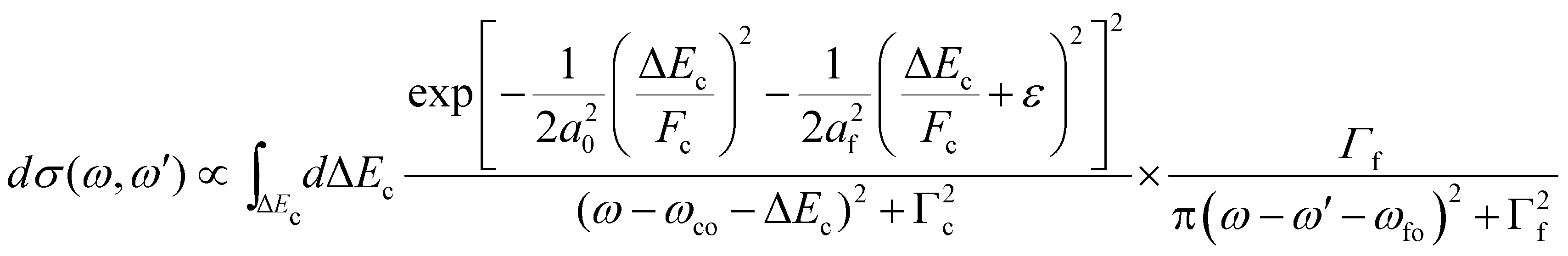
In this section, we present the equations that are necessary to simulate the 2D-maps of the resonant and normal Auger spectra, and their physical meaning. For a complete derivation of the formulas, please see ESI.†2.1 From the double differential cross section to resonant and normal Auger
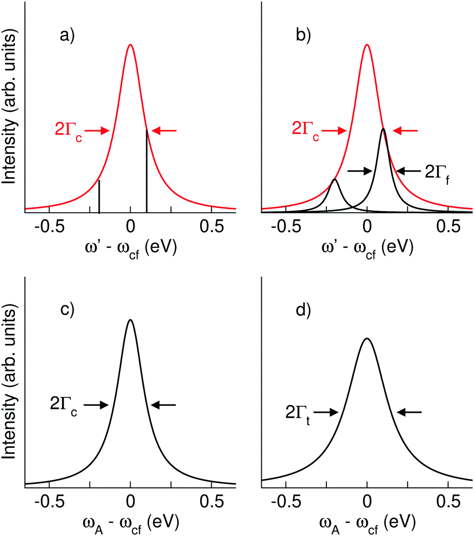
Here we describe the expected lineshapes for resonant and normal Auger spectra. Schematic pictures of these two processes are shown in Fig. 1, which also shows relevant states and energies. Here we distinguish between two cases, namely a final state with an infinite lifetime and a final state with a finite lifetime.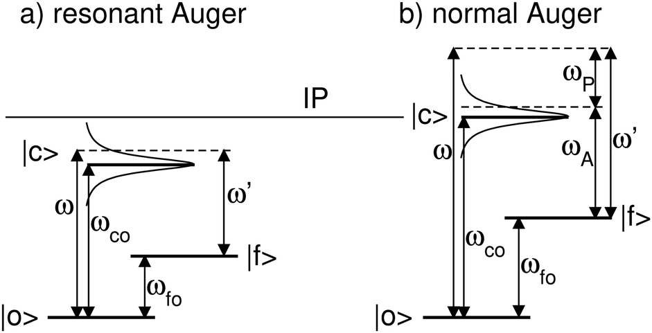 | ||
| Fig. 1 Schematics of a resonant Auger (a) and a normal Auger (b) process. |o〉, |c〉, and |f〉 indicate the ground state, the core-hole state, and the final state, respectively. ωco (ωfo) describes the energy difference between the core-hole state (final state) and ground state. ω represents the photon energy and ω′ the energy of the outgoing electrons. Note that for the resonant Auger process ω′ is equal to the kinetic energy of the Auger electron, ωA, while in case of a normal Auger process ω′ is shared between the photoelectron and the Auger electron, i.e. ω′ = ωP + ωA, with ωP being the kinetic energy of the photoelectron. For both processes the position of the ionization potential IP is also indicated. | ||
Let us start with the situation of an infinite experimental resolution and a stable final state, i.e., with infinite lifetime. In this case, the double differential cross section is described in its general form by:11
 | (1) |
 | (2) |
Eqn (1) can be used to describe both to the resonant and normal Auger processes. In the resonant Auger process in the first step an electron is excited from a core hole to an unoccupied orbital n![[small script l]](https://www.rsc.org/images/entities/char_e146.gif) below the ionization threshold. This neutral excited state can be considered as consisting of a cation A+ with an electron in the orbital n bound to it. Note that n is a counter index and describes the symmetry of the orbital; in case of an atom these quantities are equal to the principal and angular momentum quantum numbers, respectively. In the next step the cation A+ undergoes an Auger decay and forms a dication A2+ while the excited electron remains in a bound orbital. This process can be described as g.s. → A+n → A2+nε′′ with g.s. being the ground state and ε′′ being the Auger electron. In contrast to this, in the normal Auger process, the core electron is promoted in the first step into the continuum ε. Subsequently, the cation decays to a dication and emits an Auger electron. Here the process can be described as g.s. → A+ε → A2+εε′′.
below the ionization threshold. This neutral excited state can be considered as consisting of a cation A+ with an electron in the orbital n bound to it. Note that n is a counter index and describes the symmetry of the orbital; in case of an atom these quantities are equal to the principal and angular momentum quantum numbers, respectively. In the next step the cation A+ undergoes an Auger decay and forms a dication A2+ while the excited electron remains in a bound orbital. This process can be described as g.s. → A+n → A2+nε′′ with g.s. being the ground state and ε′′ being the Auger electron. In contrast to this, in the normal Auger process, the core electron is promoted in the first step into the continuum ε. Subsequently, the cation decays to a dication and emits an Auger electron. Here the process can be described as g.s. → A+ε → A2+εε′′.
In the following we shall first focus on the resonant Auger process with only one intermediate state |c〉. In this case, in eqn (2) the sum over c drops and we obtain the partial differential cross section:
 | (3) |
 | ||
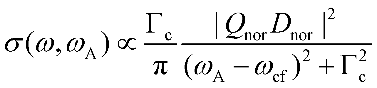
| Fig. 2 Schematic line profiles for Auger transitions. (a) Resonant Auger spectra without lifetime broadening of the final state. The spectral features are δ-functions indicated in black. The red Lorentzian curves with a width of 2Γc indicate the intensity of the δ-functions as a function of the detuning ω − ωco = ω' − ωcf. (b) Resonant Auger spectra with lifetime broadening of the final states. The black Lorentzian curves with a broadening of 2Γf represent the spectral features. For the red curve, see (a). (c) Normal Auger spectra without lifetime broadening of the final state as a function of the detuning ω − ωco = ωA − ωcf. The black Lorentzian curves with a broadening of 2Γc represent the spectral features. (d) Normal Auger spectra with lifetime broadening of the final state. The black Lorentzian curves with a broadening of 2Γt = 2(Γc + Γf) represent the spectral features. | ||
In the next step we consider the normal Auger process subsequent to a photoionization process. Note, that in the following discussion post-collision interaction (PCI) is neglected, although it is taken fully into account in our simulations, see below. In Fig. 1(b) it can be seen that the photon energy ω is not in the Lorentzian distribution of the core-hole state |c〉, i.e. the process is non-resonant. Instead, the process leads to two outgoing electrons, namely the photoelectron with a kinetic energy ωP and the Auger electron with a kinetic energy ωA. Note that ωP and ωA are the actual energies of the emitted electrons, but not the peak maxima in the photoelectron and the Auger spectrum. This leads to the relation ω′ = ωP + ωA, which can only be verified in high-resolution photoelectron-Auger electron coincidence spectra, see e.g.14 As shown in detail in the ESI† we obtain
 | (4) |
Up to now, we have assumed that the Auger final state has an infinite lifetime. This is a reasonable approximation for the Auger final states subsequent to the decay of shallow core-hole states, since in this case the final states undergo fluorescence decay which leads to much longer lifetimes. Contrary to this, the final states populated after the decay of deeper core levels (e.g. Ar 1s−1 → 2p−2) possess non-negligible lifetime broadenings which have to be taken into account. As a result, the accessible energy levels show a Lorentzian-like distribution with a width Γf around the energy of the final state; here Γf is the lifetime broadening of the final state (HWHM). Once again, we have to treat resonant and normal Auger separately.
For the resonant Auger case we obtain
 | (5) |
Obviously, the obtained result is a product of the intensity factor already present in eqn (3) and a Lorentzian function with a width Γf. From this follows that the kinetic energy of the Auger electron, ω′, can be described by a Lorentzian function with a maximum at ωfo − ω, i.e. the maximum depends on the photon energy, and a width of Γf, see black curve in Fig. 2(b). The first part on the right-hand side of the equation describes the red Lorentzian lineshape in Fig. 2(b) which indicates the intensity of the black Lorentzian curves.
In the next step we shall consider the normal Auger decay. Here we obtain
 | (6) |
As displayed in Fig. 2(d), the result of the convolution is also a Lorentzian function, however, with a larger width Γt = Γf + Γc, i.e. the sum of the lifetime broadening of the core-hole and the final state.
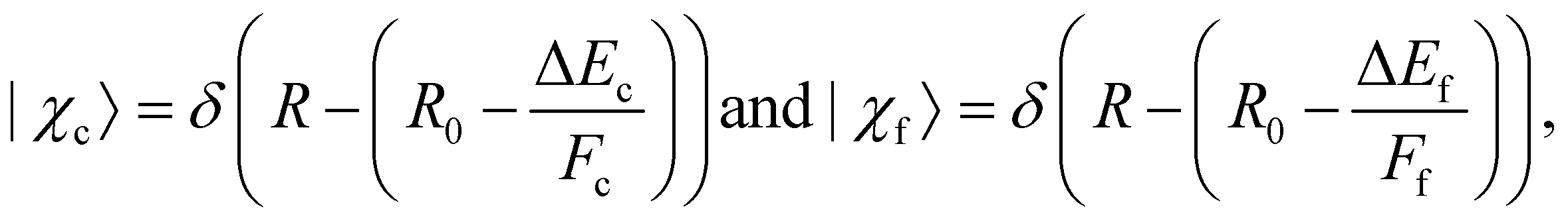
2.2 The molecular case
In this part, we discuss eqn (1) for the case of molecules with electronic and nuclear degrees of freedom, with the focus of the discussion on the nuclear degree of freedom. In the Born–Oppenheimer's approximation, we can factorize the electronic and nuclear degrees of freedom such that Ψi from the eqn (1) can be rewritten as |Ψi〉 = |Φi〉 |χi〉. |Φi〉 represents the electronic wavefunction as defined previously and |χi〉 is the nuclear wavefunction. Note that in the following we use only one vibrational wavefunction, which is equivalent to one vibrational mode and, therefore, to a diatomic molecule. However, the formulas given below can be extended to more than one vibrational mode and polyatomic molecules. In this approximation, eqn (1) can be rewritten as | (7) |
In this context Δ(ω − ω′ − ωfo, Γf) describes the spectral lineshapes and has to be derived in line with the arguments above according to the situation, i.e. resonant or normal Auger as well as the lifetime of the final states.
Let us now focus on the overlap integrals and rewrite eqn (7) with Del = 〈Φc|D|Φo〉 and Qel = 〈Φf|Q|Φc〉 as
 | (8) |
Before we continue with the discussion we want to point out that the absolute value of the sum over c can be written as
 | (9) |
The first terms on the right side of the equation are the so-called direct terms, which are sufficient when the excitation and the decay process are considered independent. In the case where excitation and decay are considered as one process, the second terms, the so-called lifetime interference terms, have to be taken into account. Here, we specify the direct terms and lifetime interference terms for the nuclear part of the wavefunctions, however, such specification is also possible for the electronic part of the wavefunctions. The most general case with vibrational and electronic lifetime interference contributions is discussed in ref. 15.
To apply eqn (8) for the vibrational states of electronic transitions, the nuclear wavefunctions χi have to be described according to the case in which they describe bound or dissociative molecular states. In principle, the transitions described by the matrix elements 〈χf|χc〉 and 〈χc|χo〉 can have different characters depending on the bond character of the potential energy curves.
In the following, we first discuss the vibrational progressions of transitions between two states, where we have to distinguish between bound–bound transitions, bound–dissociative transitions and dissociative–dissociative transitions. After this, we discuss the entire excitation and decay process, which includes three different states. Since we only consider processes which involve the ground state, we here have to distinguish four cases, namely bound–bound–bound transitions, bound–bound–dissociative transitions, bound–dissociative–bound transitions and bound–dissociative–dissociative transitions.
2.3 Transitions between two states
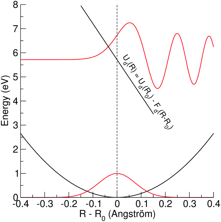 | ||
| Fig. 3 Potential energy curves in black and wavefunctions in red for a bound–dissociative transition. The lower potential energy curve and wavefunction represent the ground state of HCl in the harmonic approximation. The hypothetical upper linear potential curve has at equilibrium distance R0 of the ground state an energy of Ud(R0) ≅ 5.7 eV and a slope of −15 eV Å−1. The upper wavefunction (Airy function) is calculated for HCl based on the hypothetical potential energy curve. For more details, see text. | ||
For the calculation we assume that the slope of the dissociative potential energy curve is constant. Moreover, we assume that the bound state is the initial state and that only the vibrational ground state of the bound state is populated. By applying a harmonic oscillator potential for the bound state, the vibrational wavefunction is given by
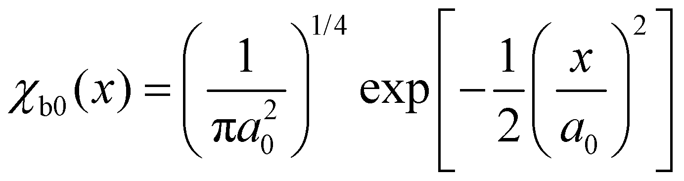 | (10) |
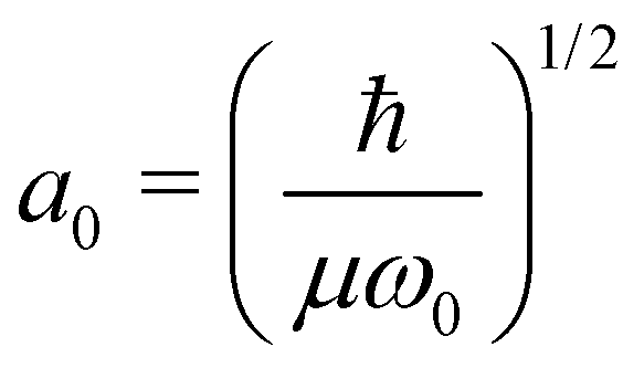 . Here, μ is the reduced mass, ω0 the vibrational frequency, and a0 the average deviation of x = R − R0 with R0 being the equilibrium distance.
As stated above, we approximate the dissociative potential energy curve with a linear function, i.e. V(x) = −Fdx with Fd being the slope of the dissociative state; The potential and the corresponding solution for one energy are displayed in the upper part of Fig. 3. The corresponding Schrödinger equation to be solved is given by:
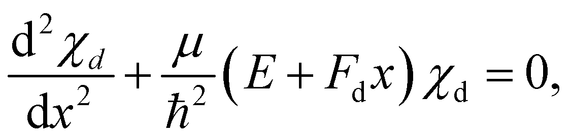 | (11) |
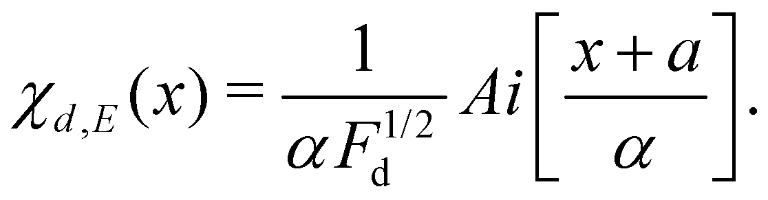 | (12) |
 ,
,  and Ai(x) being the Airy function, which is discussed in more detail in the ESI.† For
  the Airy function decreases quickly and for
  it oscillates strongly. Based on this, the Franck–Condon factors can be approximated to
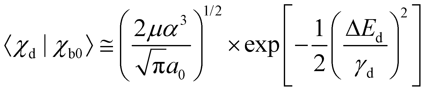 | (13) |
Obviously, the dependence of the Franck–Condon factors with the energy E can be described with a Gaussian distribution which is due to the Gaussian nuclear wavefunction in the electronic ground state. Because of this, the behavior of the Franck–Condon factors can be obtained by approximating the Airy functions by δ functions, which peak at the classical turning point. Note that in this way the energy shift Fdα can not be reproduced. One should also mention that the approximation of the Airy function by a δ function is not obvious since the width of the first oscillation of the Airy function is comparable to the width of the nuclear ground state, see Fig. 3. However, it has been shown that the Franck–Condon factors of the exact solution and the approximation deviate only very slightly, see Herzberg.20 The approximation of the Airy functions with δ functions allows also a derivation of the Franck–Condon factors for higher vibrational states in the bound potential, see e.g. ref. 21.
 | (14) |
Note that α = β if the slopes of the two potential energy curves involved are equal. This is generally assumed to be valid for Resonant Inelastic X-ray Scattering (RIXS) spectra. In this case, a nuclear wavefunction in the electronic final state is populated via one nuclear wavefunction in the initial state. As a result of a excitation and decay process, the intermediate nuclear state is always exactly known so that no vibrational lifetime interference occurs.
2.4 The entire excitation and decay process
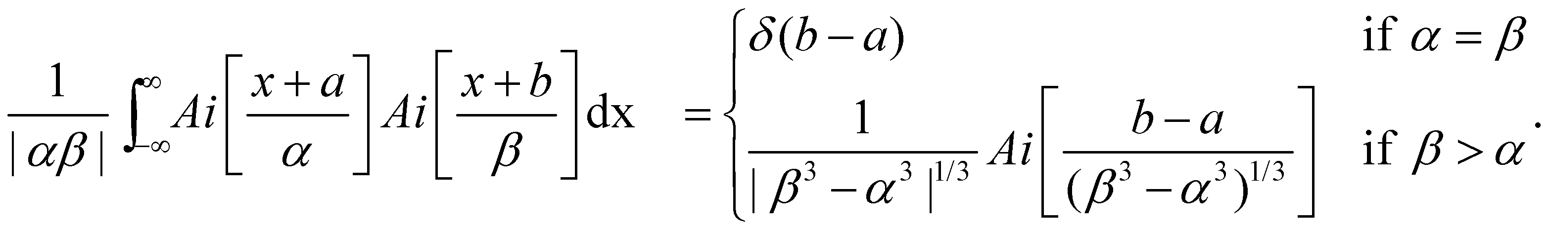
To specify the partial cross section for the given case of resonant Auger decay one has to start with eqn (8) and can use eqn (13) to replace 〈χo|χc〉. As discussed above, it was shown that for a bound–dissociative transition the Airy function can be replaced by a δ function localized at the classical turning point. We now assume for the calculation of the overlap integral 〈χc|χf〉 that this also works well for a dissociative–dissociative transition with different slopes for the potential energy curves, i.e.,
 | (15) |
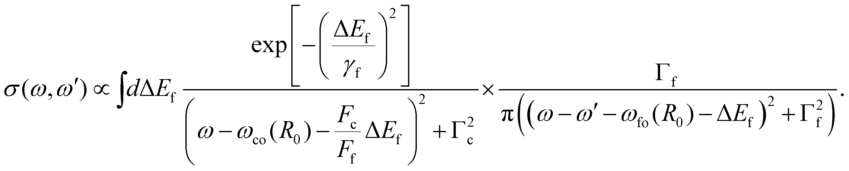 | (16) |
Here ωco(R0) and ωfo(R0) represent the energy differences between the states at the equilibrium distance R0. The integration over the different final states is represented by the integration  . Note that eqn (16) was already given in,5 however with Fc = Ff.
 . In this way, we obtain:
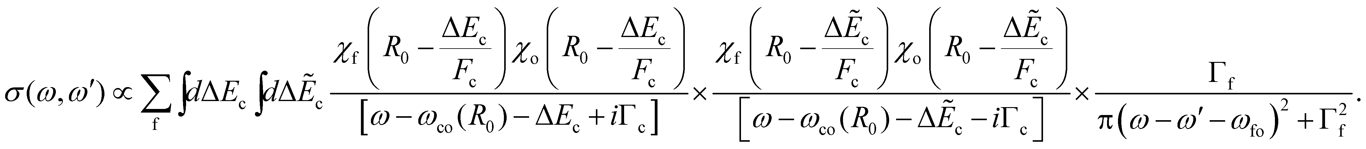 | (17) |
Here χ0(R) and χf(R) are the vibrational wavefunctions of the bound initial and final state. The integrals  and
and  replace the sums over c and c′ in eqn (9) due the continuum of levels for the nuclear motion and ensure that all possible intermediate core-excited states are taken into account.
 | (18) |
Detailed information for calculating the overlap matrix elements 〈χc|χo〉 and 〈χf|0c〉 can be found in Sections 2.3.1 and Section 2.3.2, respectively, as well as in the ESI.†
3 The influence of the experimental resolution
In Fig. 4, 2D-maps of resonant and normal KLL Auger spectra of HCl close to the Cl 1s ionization threshold are displayed. On the left side, the simulations and, on the right side, the experimental results are shown. On the x-axis, the photon energy ω and, on the y-axis, the kinetic energy of the emitted electron ω′ are displayed. In addition, the intensities of the emitted electrons are displayed by the color code. The ionization threshold can be found at ≅ 2830 eV, i.e. below this photon energy resonant Auger spectra and above this value normal Auger spectra as well as electron recapture processes can be observed. An integration along the kinetic-energy axis leads to a partial-electron-yield spectrum, which compares to an absorption spectrum in this energy region. The corresponding spectra are shown above each map. A direct comparison of the experimental and the theoretical absorption spectrum is presented in the ESI.† The absorption spectra allow identifying the intermediate core-hole states. The final states of the displayed transitions can be identified by comparing with Fig. 6 to 10 below.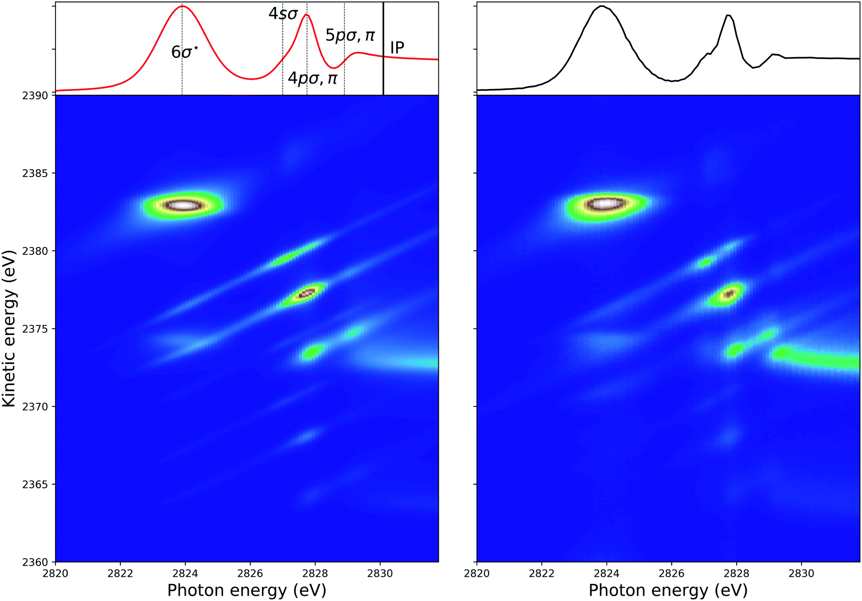 | ||
| Fig. 4 The simulated (left) and the experimental (right) 2D-map. Above each map, the corresponding partial-electron-yield spectra are given, which also allows to identify the core-hole states. Both, the theoretical and experimental partial-electron yield spectra were obtained by projecting the 2D-maps on the photon-energy axis. For the identification of the final states of the different spectral contributions, see Fig. 6 to 10 below. | ||
In the maps, the normal Auger transition Cl 1s−1 → 2p−2(1D) is represented by the almost horizontal line at 2373 eV kinetic energy. The resonant Auger transitions below threshold mostly show inclined lines, which represent resonant Auger transitions to stable or metastable final states. The strong horizontal line around a photon energy of 2824 eV and a kinetic energy of 2383 eV is due to the Cl 1s−16σ → 2p−2(1D)6σ. Here, both states are strongly dissociative and the horizontal orientation of the spectral feature is a signature of ultrafast nuclear dynamics.24
The spectral features can be described by the formulas given above, which, however, do not take into account the experimental resolution consisting of the photon bandwidth and the detector resolution. To obtain simulated maps that can be compared with the experimentally observed 2D-maps, the theoretical maps have to be convoluted with the photon bandwidth along the photon energy axis and with the detector resolution along the electron kinetic energy.
In the following, we discuss how these convolutions along different directions contribute to the spectra, which are present or can be derived from the 2D-map. As already stated above, an integration along the kinetic-energy axis is comparable to the photoabsorption spectrum. In this case, and because the photon bandwidth and instrumental resolution can be defined by normalized Gaussian functions, the detector resolution cancels out so that only the convolution with the photon bandwidth contribute to the absorption spectrum. Normal Auger spectra far above threshold lead to horizontal lines, i.e. do not depend on the photon energy. Because of this only the detector resolution has to be taken into account.
As discussed by Guillemin et al.8 the situation becomes more complicated close to the ionization threshold. In this region, the energy position and the lineshape are influenced by PCI and depend, as a result, on the photon energy. This can be seen by the almost horizontal line visible above threshold at a kinetic energy of ≅ 2373 eV, which is slightly bent towards higher kinetic energies while approaching the threshold. As a consequence of this photon-energy dependent peak position due to PCI, the Auger spectra become – at least in principle – also dependent on the photon bandwidth. Therefore, in a rigorous treatment, the simulated Auger lines have to be convoluted as discussed above. For normal Auger spectra close to threshold a simplified way is described by Guillemin et al.8 In this case, the PCI lineshape can be convoluted with the detector resolution and a modified photon bandwidth γ′ = |m| × γ with  . Here ΔEPCI is the PCI-shift and Eex the kinetic energy of the photoelectron. Note that m is usually small and the resulting resolution can be neglected.
Although not visible in the present case, the emission of a photoelectron causes a diagonal line with a slope of m = 1 in a 2D-map. Because of this, a photoelectron line has to be convoluted with both the photon bandwidth and the detector resolution. Finally, we discuss the lines caused by resonant Auger transitions to different final states, which also show a dispersion with photon energy. This dispersion is linear with a slope of m = 1, i.e., results in diagonal lines, with the exception of dissociative final states in the vicinity of the resonance position. Although in this case, the slope is identical to that for a photoemission process, the resonant Auger lines have to be treated differently because of two reasons. First, the core-hole lifetime does not contribute to the lineshape, see above, and second, the cross section varies strongly with the photon energy, see Fig. 2. Therefore, the lineshape in a resonant Auger spectrum can be obtained by multiplying the Lorentzian curve in Fig. 2 with the Gaussian distribution for the photon bandwidth; note that this can lead in the case of broad photon bandwidths to asymmetric lineshapes.25,26 Finally, the result has to be convoluted with the detector resolution.
4 Results and discussion
4.1 Computation of the potential energy curves
The potential energy curves shown in Fig. 5 were computed using the MOLPRO package27 at the CASSCF level. We chose the Gaussian basis set aug-cc-pCVTZ,28,29 in order to take into account core–core and core–valence correlation effects, and included scalar relativistic corrections using the Douglas–Kroll Hamiltonian,30–32i.e. spin–orbit interaction is neglected.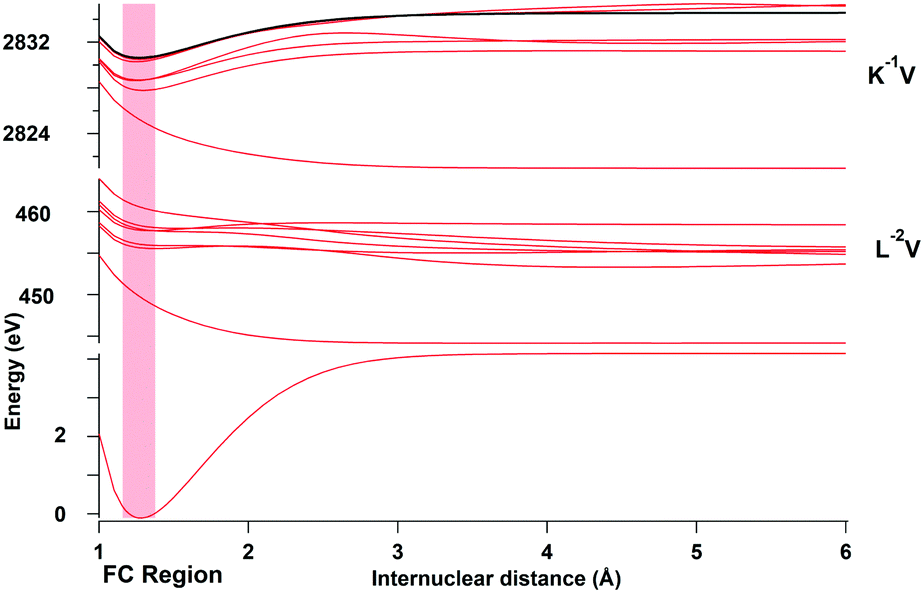 | ||
| Fig. 5 Calculated potential energy curves for the ground state, the intermediate Cl K−1V core-hole states and Cl L2,3−2(1D)V double core-hole final states. The potential energy curve of the K−1 ionic state is represented in black. The Franck–Condon region is indicated by the shaded vertical region. | ||
In the present study, the 15 lowest singly excited Cl 1s−1 states were calculated and only those states which were observed experimentally in ref. 10 are represented in Fig. 5. In this figure, three distinct regions corresponding to the different types of electronic states populated in the entire excitation and resonant Auger process are visible: the ground state at low energies, the K−1V region around 2824 eV, which corresponds to the core-excited states, and the L−2V region around 450 eV, which corresponds to the Auger final states. In addition, the potential curve of the ionized K−1 state is represented by the black line and the Franck–Condon (FC) region is indicated by a red-shaded area.
The lowest potential energy curves in each of the regions K−1V and L−2V are highly dissociative and correspond to the states K−16σ and L−26σ, respectively. These states have attracted substantial interest in the literature3,4,10,24 since they lead to ultrafast nuclear motion and even show indication of ultrafast dissociation.
Also of interest is the bond character of the L−2Ryd states where Ryd indicates a Rydberg orbital. In first approximation the bond character of these states can be estimated on the exotic Z + 2 molecule HK2+, which suggests a dissociative character. Nevertheless, some of these final states are meta-stable with a shallow potential well like L−24sσ or L−23dσ and other (L−24pσ,π and L−24pσ,π) are dissociative. A similar behavior was found for the O K−2Ryd states in CO,33 which can be compared with the molecule CNe2+. From these results we conclude that double-core-hole Rydberg excitations tend to be close to the borderline between metastable and dissociative so that each state has to be individually considered.
To obtain simple analytical expressions, which allow analytical treatments of the vibrational part of the transitions, the potential energy curves were fitted using the model potential functions as described in Gortel et al.34 All potential energy curves with a minimum in the Franck–Condon region were fitted to a Morse potential. Note that in particular the L−2V states show at large distances strong deviations from the Morse potential. Because of this, the fits of the potential were only performed close to the Franck–Condon region, which is relevant for the transitions.
The dissociative states were fitted by the exponential decay form
| V(R) = Ve(V′/V)(R−R0) + V∞ | (19) |
4.2 Parameters used in the simulations
The energy positions of the various excited states relative to the ground state and the Auger energies for the transitions to the studied final states are summarized in Table 1. As mentioned in ref. 10, we observe resonant Auger transitions to two groups of final states, namely the 2p−2(1D)V and 2p−2(1S)V. The notation corresponds to the spectroscopic term for the equivalent atomic notation with two holes in the 2p shell and one electron in a high-energy molecular orbital, which is denoted by V and is unoccupied in the ground state. The transitions to the 2p−2(3P)V final states states are too weak to be observed.| Excited electronic state | Energy (eV) |
|---|---|
| 1s−16σ | 2823.90 |
| 1s−14sσ | 2827.05 |
| 1s−14pσ,π | 2827.75 |
| 1s−15pσ,π | 2828.90 |
| 1s−1 | IP = 2830.10 |
| Final electronic state | Kinetic energy for spectator decays (eV) |
|---|---|
| 2p−2(1D)6σ | 2382.9 |
| 2p−2(1D)4sσ | 2379.5 |
| 2p−2(1D)4pσ,π | 2377.3 |
| 2p−2(1D)5pσ,π | 2374.5 |
| 2p−2(1D) | 2372.3 |
| 2p−2(1S)6σ | 2374.2 |
| 2p−2(1S)4sσ | 2370.3 |
| 2p−2(1S)4pσ,π | 2368.1 |
| 2p−2(1S)5pσ,π | 2365.3 |
| 2p−2(1S) | 2363.3 |
To compare the obtained simulations better with the experimental data of ref. 10, we convoluted our results with two normalized Gaussian functions with a full width at half maximum (FWHM) of 0.22 eV and 0.30 eV, in order to simulate the detector resolution and photon bandwidth, respectively. The lifetime broadenings (FWHM) were chosen as 2Γc = 0.65 eV for the 1s−1V excited states35 and 2Γf = 0.24 eV for the 2p−2V final states.3
Finally, for our simulations, we applied for the Auger transitions to the 2p−2(1D)V and the 2p−2(1S)V states the same parameters, with two exceptions. First, we used different kinetic energies for the Auger electrons as stated in Table 1. And second, we applied a 2p−2(1S)V to 2p−2(1D)V intensity ratio of 0.1; this ratio has been observed for the diagram lines in argon6 and it is expected to vary only slightly with the atomic number Z so that the value for argon can be used as good approximation for Cl.
4.3 Details of the simulations of the bound–bound–bound, the bound–bound–dissociative and bound–dissociative–bound transitions
In the simulations, some of the excitation and decay processes were treated as bound–bound–bound transitions, see Section 2.4.1. The parameters R0, ħω, and xħω for the ground state of the molecule can be obtained from literature. The parameters for the core-hole state and the final state can either be derived from a fit of the photoelectron and the Auger spectrum, respectively, or from a fit of the calculated potential energy curves to the Morse formula, see Section 4.1. The final states are not really stable but metastable since for large distances the Coulomb repulsion becomes important. However, if the inner well of such a potential is deep enough, a Morse potential is a good approximation, see e.g. ref. 38 and 39.In the following we shall discuss the calculations for HCl in more detail. Here, we are interested in the Cl 1s−1 photoabsorption process and the subsequent resonant Auger decay to the 2p−2nl final states. As discussed above, for this we have to calculate in principle the overlap matrix elements 〈χf|χc〉 and 〈χc|χo〉. As can be seen from Fig. 5, the Cl 1s−1Ryd states and the Cl 1s−1 ionic state are stable according to our calculations. This is not surprising since their potential energy curves are expected to be very similar to the HCl 2p-hole states. This is due to the fact that potential energy curves are determined by the valence electrons, not by the core holes. The 2p−1 states are known to be bound also from experiment, see e.g. for photoabsorption ref. 40 and for photoemission ref. 41. The spectra in the latter two references show practically only transitions to the vibrational ground state of the core-hole state, while transitions to higher vibrational substates are almost absent. From this follows that matrix element | 〈0c|0o〉 |2 ≅ 1 while the matrix elements | 〈nc|0o〉 |2 ≅ 0 for n > 0. Because of this, only the vibrational ground states in the core-hole states are taken in our simulations into account. This also leads to the fact that vibrational lifetime interference can be neglected.
To calculate the Franck–Condon factors | 〈χf|0c〉 |2 for the resonant Auger transitions, the potential energy curves of the Cl 1s−1 core-hole and the Cl 2p−2 final states were fitted to a Morse potential. Since the Cl 1s−1Ryd states are all stable, the fit is performed over the entire region of internuclear distances. Contrary to this, the 2p−2Ryd are only metastable. Because of this we use for the fit only the region of 1 to 2 Å for the internuclear distances in order to approximate the states with a Morse potential.
In case of large changes in the internuclear distances and/or very shallow wells for the Morse potentials, transitions to the continuum wavefunctions for the nuclear motion are possible, i.e. in these cases both bound–bound and bound–dissociative transitions, occur. Since for Auger final states the dissociation energy of Morse potentials is normally larger than the potential energy barrier of the potential energy curve, see ref. 38 and 39 we utilized the above-described approach only for these transitions, for which we obtained that at least 70% of the transitions end in a bound vibrational state. All other transitions are described as with bound–dissociative transitions.
In the next step, we shall discuss the bound–bound–dissociative transitions. These transitions are relevant for some of the Cl 1s−1Ryd → 2p−2Ryd transitions. Due to the fact that | 〈 0c|0o〉 |2 ≅ 1, we can simplify eqn (18) with eqn (10) to
 | (20) |
Now let us turn to the bound–dissociative–bound transitions, which are realized for the Cl 1s−16σ → 2p−24sσ and Cl 1s−16σ → 2p−23dσ shake-up transitions. For these transitions, eqn (17) has to be applied. Here the vibrational wavefunction for the electronic ground state χo(R) can be described in good approximation with that of the harmonic oscillator.
4.4 Results of the simulations and comparison with experiment
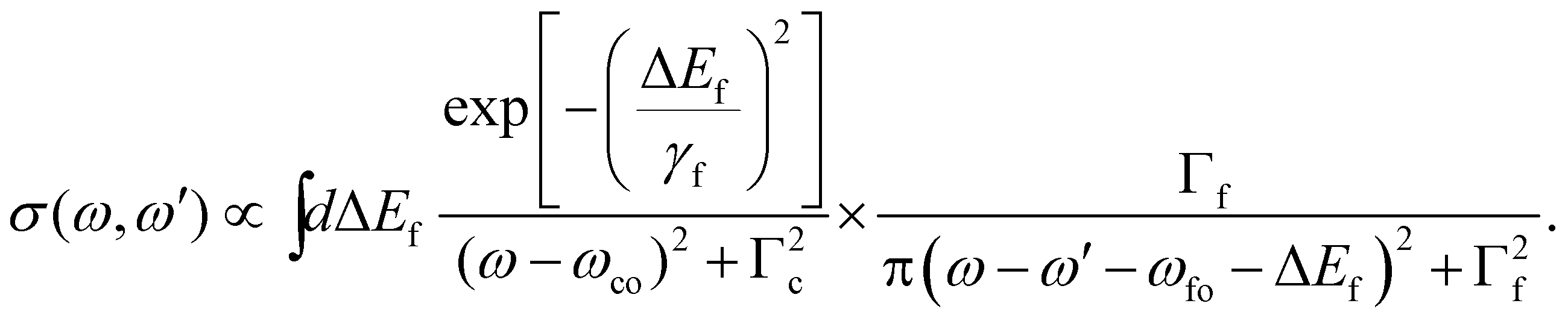
In the following, we describe the results on each final state. Actually, we performed two types of simulations, namely first the simulations of the entire map, see Fig. 4, and with this the contributions of each individual final state to the map, see below. Second, we simulated final-state cross sections, which give the probability for a population of a given final state of the type 2p−2V as a function of the photon energy. Experimental final-state cross sections can be obtained by plotting the intensities along the diagonal lines in the measured 2D-map as a function of the photon energy. Note that throughout this work we give only relative cross sections, but not absolute values. Nevertheless, for reasons of simplicity we use the term cross section. Details on the analysis and simulation of final-state cross sections including electronic state lifetime interference are presented in ref. 9, 10. The present experimental data are identical to those presented by Goldsztejn et al.,10 however, two of the final-state cross sections, namely those for the 2p−25pσ,π and the 2p−23dσ are presented for the first time. The data are recorded using a detection direction parallel to the polarisation direction of the synchrotron radiation, but not at magic angle. This leads to an angular dependence of the individual resonance intensities, i.e., we expect intensity ratios which are slightly different from those expected at magic angle. This is, however, a minor point in the present work since we do not compare our fitted intensities with calculated ones. Note, that a comparison of exerimental and theoretical results can be performed directly if the angular distribution of the Auger electron is taken into account. Nevertheless, we prefer to use in the present publication for the experimental results the term pseudo-cross section rather than partial cross section. Then, we first present the results for the dissociative final states and after this for the bound final states.Final state 2p−26σ. The left side of Fig. 6 displays the experimental (black data points) and simulated (red line) cross sections of the final electronic state 2p−26σ. The dashed black lines below the cross sections represent the direct terms of the dominant 1s−16σ → 2p−26σ spectator Auger decay as well as shake transitions from the 1s−14sσ intermediate state. Note that in the simulated cross sections shown in Fig. 6 to 10, electronic lifetime interference contributions are included, see ref. 10; however, these contributions are only shown in Fig. 7 as individual lines in order to keep the number of dashed lines in the other Figures small.
 | ||
| Fig. 6 Cross section of the 2p−26σ (left) as a function of the photon energy, the black dots are the experimental points and the solid line is the result of our simulation. The dashed lines in the lower part of the figure display the contributions of the individual intermediate states. The simulated contributions of this final state to the 2D-map are displayed on the right-hand side of the figure. | ||
 | ||
| Fig. 7 Cross section of the 2p−24pσ,π (left) as a function of the photon energy, the black dots are the experimental points and the solid line is the result of our simulation. The dashed lines in the lower part of the figure display the contributions of the individual intermediate states. The solid blue, green and black lines represent the electronic lifetime-interference contributions, for details see text. The simulated contributions of this final state to the 2D-map are displayed on the right-hand side of the figure. | ||
To simulate the cross section of the 2p−26σ final state, we considered the relaxation to this state from the 1s−16σ intermediate state, which corresponds to the spectator decay, shake-downs from the orbitals 4sσ, 4pσ,π and 5pσ,π as well as a recapture after 1s ionization. Following ref. 42, one can define the modulus squared of the overlap integral  as a probability of recapture, where β is a slowly varying function of energy and Eexc is the excess energy.
The result of our simulation is shown on the left side in Fig. 6 as a red solid line, together with black dots corresponding to the experimental data points. The dashed lines below the graph indicate the individual contributions from the different 1s−1V excited states.
Both the 1s−16σ intermediate and the 2p−26σ final state are dissociative so that we simulated this transition with eqn (16). As clearly visible in Fig. 6, this transition is highly dominant in this final-state cross section. Its broad Gaussian-like shape originates from the highly dissociative character of the potential curve of the excited state 1s−16σ with a slope of Fc = −9.27 eV Å−1 at the ground state equilibrium distance R0 = 1.27 Å; this slope agrees reasonably well with the value of −10.2 eV Å−1 given by Travnikova et al.3 The only other visible contribution is a shake-down from the 4sσ orbital. The 1s−14sσ excited state is bound and we therefore used for the simulation eqn (20), which describes bound–bound–dissociative transition.
The slope of the potential energy curve of the intermediate state 1s−16σ at the equilibrium distance is relevant to fit the final-state cross section, see above. However, to reproduce well also the resonant Auger spectra, and with this the shape in the 2D-map, the slope of the 2p−26σ final state has to be taken into account, see eqn (16). However, for the best agreement between experiment and theory we had to use a slope of the potential energy curve of Ff = −11.77 eV Å−1. This slope has been calculated for an internuclear distance of ≈R0 + 0.1 Å and not for R0 as used in eqn (16). This difference in the internuclear distance is probably due to the propagation of the wavepacket in the intermediate state prior to its projection on the final-state nuclear wavefunctions.
We show the result of this simulation also on the right side of Fig. 6, where one can observe two spectral contributions. One shows a linear dispersion with the photon energy, which is due to the kinetic energy conservation part of the Lorentzian function of the eqn (16) as discussed in detail above. The other contribution displays in the resonance region a non-linear dispersion, which corresponds to strongly dissociative intermediate and final states. The exact shape of this non-linear dispersion depends on the ratio of the two potential slopes, as can be understood from the eqn (16). These two contributions are also present in the experimental 2D-map, which is visible on the right side of the Fig. 4.
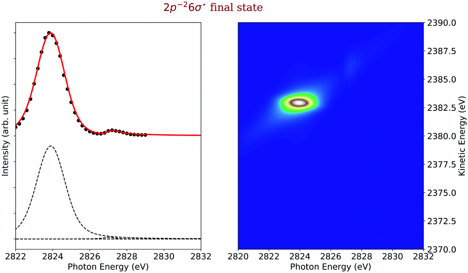
Final states 2p−24pσ,π. The left side of Fig. 7 displays the experimental (black data points) and simulated (red line) cross sections of the final electronic states 2p−24pσ,π. The dashed black lines below the cross sections represent the direct terms of the dominant 1s−14pσ,π → 2p−24pσ,π spectator Auger decay as well as shake transitions from other intermediate states. The blue, green and black solid lines represent the electronic lifetime-interference contributions. In detail, the blue line represent the contributions caused by the interference between the 1s−16σ and the 1s−14pσ intermediate states, the green line between the 1s−14pσ,π resonant and the 1s−1 continuum intermediate states, as well as the black curve between the 1s−14pσ,π and 1s−15pσ,π intermediate states.
The intermediate 1s−14pσ,π electronic state is bound, i.e., the entire excitation and decay process is of the type bound–bound–dissociative and can be described with eqn (20). Since this main decay channel implies a bound intermediate state, no nuclear dynamics can be observed in the Auger spectra and only linearly dispersive contribution are visible in the respective 2D-map, see right hand side of Fig. 7. The second clearly visible contributions to the 2p−24pσ,π cross section originates from a transition from the 1s−16σ intermediate state and includes a shake-up process of the excited electron. The corresponding process is of the type bound–dissociative–dissociative. Because of this, nuclear dynamics can occur in the intermediate state. This is reflected in the 2D-map of Fig. 7 in the energy range around the 1s−16σ resonance energy by a slope slightly different from one.
The final-state cross section also shows a small contribution from a shake-down process involving the 1s−15pσ,π electronic state. As can be seen by the black dashed lines and the black solid line, the electronic lifetime-interference contribution caused by the 1s−14pσ,π and 1s−15pσ,π intermediate state is more intense than the contribution of the 1s−15pσ,π direct terms. These electronic lifetime-interference contributions are responsible for the weakly pronounced minimum of the cross section at a photon energy of ≅ 2828.5 eV and can also be seen in the experimental results with an increase of the intensity with the last data point. Such effects cause by lifetime interference are typical for cases with one very intense and one very weak direct term, compare, e.g., ref. 15, 23. This minimum is even more clearly visible in the 2D-map where one observes an intensity “hole” slightly below the photon energy of hν = 2829 eV. Finally, there are two more very weak contributions of approximately the same peak intensity, namely a shake-up after the passage through the 1s−14sσ intermediate state and from a recapture of the photoelectron emitted during 1s ionization.
Final states 2p−25pσ,π. The cross sections of the final states 2p−25pσ,π are shown on the left-hand side of Fig. 8 and reveal contributions from three different intermediate states. The most intense one is due to a shake-up from the 1s−14pσ,π intermediate electronic state. This is due to the fact that the increasing positive charge seen by the excited state orbital, namely +1 in the core-hole state and +2 in the Auger final state, leads to a shrinking of the orbitals and, therefore, to strong shake-up transitions, see e.g. ref. 43. The second most intense transition comes from a recapture of the photoelectron emitted during the ionization process. This recapture depends on the overlap of the continuum wavefunction of the photoelectron and the excited final-state orbital (here 5pσ,π). The third contribution to this final-state cross sections is the spectator decay corresponding to a 1s−15pσ,π → 2p−25pσ,π transition. All of these transitions are bound–bound–dissociative.
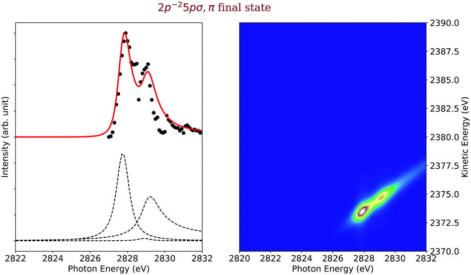 | ||
| Fig. 8 Cross section of the 2p−25pσ,π (left) as a function of the photon energy, the black dots are the experimental points and the solid line is the result of our simulation. The dashed lines in the lower part of the figure display the contributions of the individual intermediate states. The simulated contributions of this final state to the 2D-map are displayed on the right-hand side of the figure. | ||
Final state 2p−24sσ. On the left side of Fig. 9, we represented in black the experimental data points and as red solid line the simulated cross sections of the 2p−24sσ final state, along with the direct terms contributing to the cross section, which are indicated by dashed black lines. In the final-state cross section, three main contributions are visible, namely the spectator decay of the 1s−14sσ state, a shake-down process from the 1s−14pσ state and a shake-up process after excitation to the 1s−16σ excited state. In the first two cases, the excited states are bound so that the entire process can be considered bound–bound–bound as described in Section 2.4.1. The situation is more complex for the case of the shake-up from the LUMO orbital that involves a dissociative intermediate state.
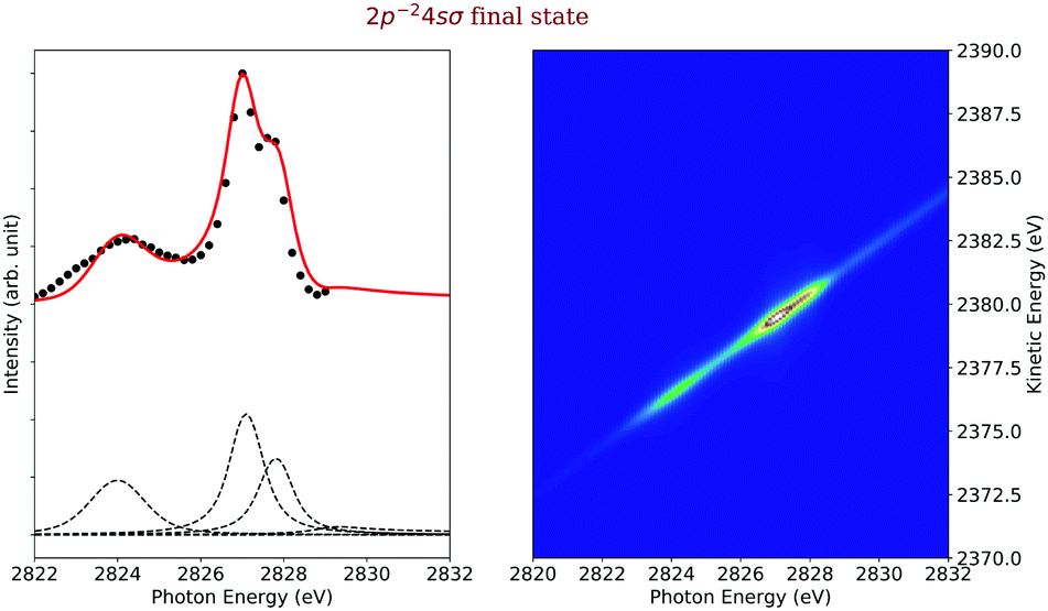 | ||
| Fig. 9 Cross section of the 2p−24sσ (left) as a function of the photon energy, the black dots are the experimental points and the solid line is the result of our simulation. The dashed lines in the lower part of the figure display the contributions of the individual intermediate states. The simulated contributions of this final state to the 2D-map are displayed on the right-hand side of the figure. | ||
As described in the Section 2.4.3, to calculate the overlap matrix element for the nuclear wavefunctions of the dissociative intermediate and the bound final state, generalized Laguerre polynomials have to be applied.44 Therefore, the cross section has to be calculated in a time-consuming manner numerically by applying a double integration over the vibrational states populated. Because of this, we used a simplified approach of eqn (17) by making two approximations. First, we neglected vibrational lifetime interference by using only the direct terms and second, we assumed a harmonic oscillator potential for the final state and populated only the vibrational ground state. Actually, the final state has several vibrational levels and we shifted the energy position to the center of the positions of the first five vibrational levels. In this way, we obtained the simplified cross section
 | (21) |
Final state 2p−23dσ. The experimental and simulated cross sections of the 2p−23dσ final state are shown on the left-hand side of Fig. 10 as black dots and red line, respectively. Interestingly, this final state can only be accessed through shake processes but not by a spectator decay via the 1s−13dσ state since such excitations are not present in the absorption spectrum; this excitation is expected to be located approximately 1.5 eV above the 1s−14sσ state,45 but no features are visible in this region of the spectrum. This observation may be explained as follows: in the core-excited state the 3dσ Rydberg orbital is still rather atomic-like so that the dipole selection rules for atoms explain the absence of this excitation in the absorption spectrum. In the final state, the 3dσ orbital becomes smaller due to the higher charge caused by the two core holes. In this way, it obtains a stronger valence character and mixes with other orbitals of the same symmetry. As a result, the monopole selection rules for shake transitions can explain the population of this final state.
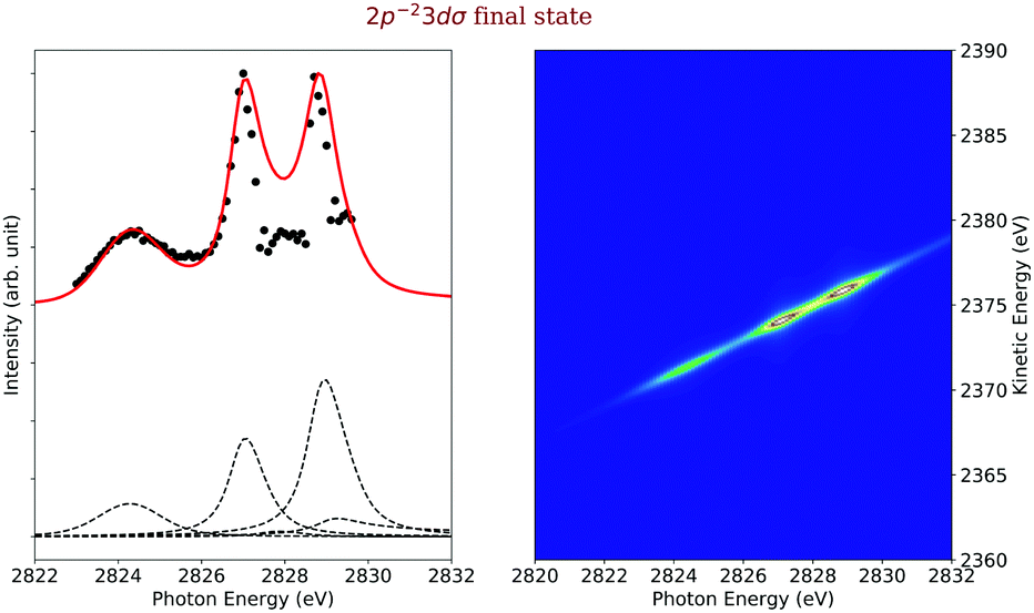 | ||
| Fig. 10 Cross section of the 2p−23dσ (left) as a function of the photon energy, the black dots are the experimental points and the solid line is the result of our simulation. The dashed lines in the lower part of the figure display the contributions of the individual intermediate states. The simulated contributions of this final state to the 2D-map are displayed on the right-hand side of the figure. | ||
The main contributions to this final state are indicated by dashed vertical lines below the cross section, see Fig. 10. Two of the contributions are caused by shake-up processes, namely from the 1s−16σ and 1s−14sσ excited states, and two more by a shake-down process from the 1s−15pσ excited state and recapture from the singly ionized state. Due to its weak intensity and its proximity to other final states in the 2D-map, see Fig. 4, it was very challenging to extract the experimental pseudo-cross section from the map. However, we believe that the overall agreement between the experimental and the simulated cross section is fairly good. The largest discrepancies occur at ≈ 2828 eV, which is the region with the strongest overlap with the more intense transitions to the final state 2p−25pσ,π, see Fig. 4, so that the extraction of the 2p−23dσ cross section was very difficult and not highly accurate.
The two most intense contributions to this final state cross section are due to the shake processes from the 1s−15pσ,π and 1s−14sσ intermediate states. Both these intermediate states are bound and therefore the entire process is described as a bound–bound–bound one. For the contributions via the 1s−16σ intermediate state we applied again eqn (21) since the entire process represents a bound–dissociative–bound case. Finally, although the intensity of the direct term involving a recapture of an emitted photoelectron onto the 3dσ orbital is not strong, its interference terms, in particular with the terms involving the 4sσ and 5pσ,π orbitals, are very important to lower the intensity of the simulated curve in the energy region between the 1s−14sσ and the 1s−15pσ,π.
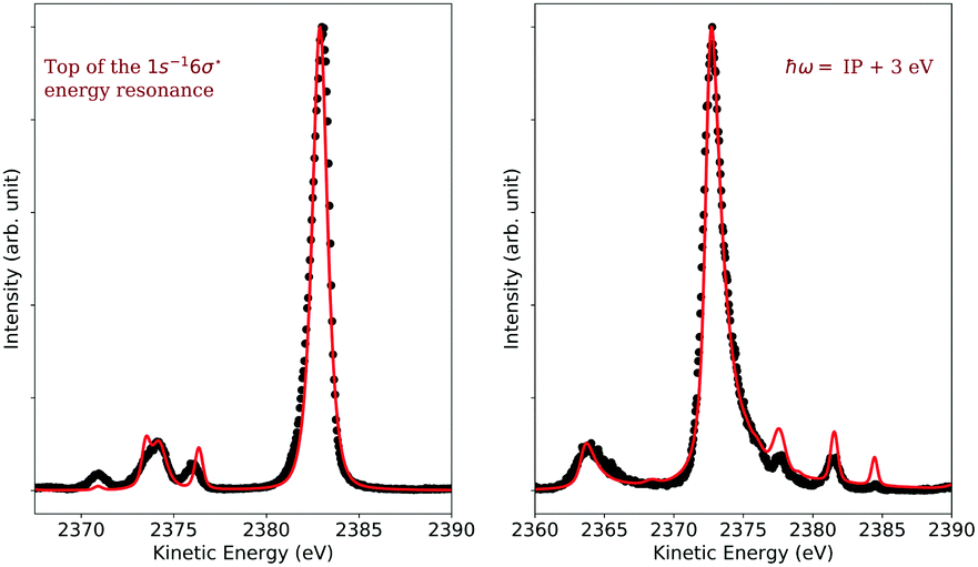 | ||
| Fig. 11 Left: Resonant Auger spectrum recorded at the resonance energy of the 1s−16σ transition. The black dots represent the experimental data and the red solid line the simulation. Right: Experimental normal Auger spectrum measured at ħω = IP + 3 eV (black dots) along with the corresponding simulated spectrum (red line). In both cases, the spectra were normalized to one. | ||
5 Summary and conclusions
In previous studies, experimental 2D-map consisting of resonant Auger spectra obtained at different photon energies were mostly investigated by considering only partial aspects. In this context, often the core hole to LUMO excitations are in the focus of publications since they allow to investigate ultrafast nuclear motion along dissociative potential energy curves. In contrast to this, in the present work we analyzed the 2D-map as a whole and paved the road towards a comprehensive understanding of such 2D-maps. For this purpose, we compiled the present understanding of all theoretical aspects that are necessary and simulate an experimental 2D-map consisting of Auger spectra obtained at different photon energies.We applied the presented theory to simulate the 2D-map of HCl close to the Cl 1s−1 ionization threshold and found good agreement with experimental data. Such an approach allows to separate overlapping spectral contributions and gives, therefore, deeper understanding of the electronic and nuclear dynamics reflected in the maps. In the present case we found generally good agreement between simulations and experiment. However, we also found disagreement in some minor points, which indicates that the spectrum is not yet understood in full detail. These differences are most probably due to simplifications in the applied theoretical framework. As an example, in the Auger case, i.e., in bound–dissociative–dissociative processes with different slopes for the intermediate and the final state, the contributions of vibrational lifetime interference was neglected. Since such contributions cannot strictly be ruled out, it might be necessary to investigate possible influences of vibrational lifetime interference in more detail. However, the differences might also be due to effects, which are not yet realized to be present or underestimated in such 2D-maps. However, these topics are beyond the scope of the present work.
The next natural step would be an implementation of the theoretical framework in a 2D-fit approach. This would allow to investigate regions with strongly overlapping contributions, like in the present case close to threshold, or for other molecules with more complex electronic structures. In near future, we also expect 2D-maps with significantly higher experimental resolution to provide more detailed information, since new high-resolution monochromators in the HAXPES regime are now available, providing a photon energy resolutions of E/ΔE of almost 50.000 at 7 keV.46 2D-Maps measured with such high experimental resolution will reveal in particular in the resonant Auger region much finer details and will provide a benchmark for theoretical descriptions.
In summary, we believe that the present approach is an important step towards a more effective data analysis of 2D-maps of Auger spectra close to deep core holes, both for atoms and molecules.
Conflicts of interest
There are no conflicts to declare.Acknowledgements
Experiments were performed on the GALAXIES beamline at SOLEIL Synchrotron, France (Proposals No. 20120122 and 20130309). We are grateful to D. Prieur for technical assistance and to SOLEIL staff for smoothly running the facility.Notes and references
- M. N. Piancastelli, T. Marchenko, R. Guillemin, L. Journel, O. Travnikova, I. Ismail and M. Simon, Rep. Prog. Phys., 2020, 83, 016401 CrossRef CAS PubMed.
- L. Journel, R. Guillemin, A. Haouas, P. Lablanquie, F. Penent, J. Palaudoux, L. Andric, M. Simon, D. Céolin, T. Kaneyasu, J. Viefhaus, M. Braune, W. B. Li, C. Elkharrat, F. Catoire, J.-C. Houver and D. Dowek, Phys. Rev. A: At., Mol., Opt. Phys., 2008, 77, 042710 CrossRef.
- O. Travnikova, T. Marchenko, G. Goldsztejn, K. Jänkälä, N. Sisourat, S. Carniato, R. Guillemin, L. Journel, D. Céolin, R. Püttner, H. Iwayama, E. Shigemasa, M. N. Piancastelli and M. Simon, Phys. Rev. Lett., 2016, 116, 213001 CrossRef PubMed.
- O. Travnikova, N. Sisourat, T. Marchenko, G. Goldsztejn, R. Guillemin, L. Journel, D. Céolin, I. Ismail, A. Lago, R. Püttner, M. N. Piancastelli and M. Simon, Phys. Rev. Lett., 2017, 118, 213001 CrossRef CAS PubMed.
- T. Marchenko, G. Goldsztejn, K. Jänkälä, O. Travnikova, L. Journel, R. Guillemin, N. Sisourat, D. Céolin, M. Žitnik, M. Kavčič, B. Cunha de Miranda, I. Ismail, A. F. Lago, F. Gel’mukhanov, R. Püttner, M. N. Piancastelli and M. Simon, Phys. Rev. Lett., 2017, 119, 133001 CrossRef CAS PubMed.
- R. Püttner, P. Holzhey, M. Hrast, M. Žitnik, G. Goldsztejn, T. Marchenko, R. Guillemin, L. Journel, D. Koulentianos, O. Travnikova, M. Zmerli, D. Céolin, Y. Azuma, S. Kosugi, A. F. Lago, M. N. Piancastelli and M. Simon, Phys. Rev. A, 2020, 102, 052832 CrossRef.
- V. Schmidt, Rep. Prog. Phys., 1992, 55, 1483 CrossRef CAS.
- R. Guillemin, S. Sheinerman, R. Püttner, T. Marchenko, G. Goldsztejn, L. Journel, R. K. Kushawaha, D. Céolin, M. N. Piancastelli and M. Simon, Phys. Rev. A: At., Mol., Opt. Phys., 2015, 012503, 92 Search PubMed.
- G. Goldsztejn, R. Püttner, L. Journel, R. Guillemin, O. Travnikova, R. K. Kushawaha, B. Cunha de Miranda, I. Ismail, D. Céolin, M. N. Piancastelli, M. Simon and T. Marchenko, Phys. Rev. A, 2017, 95, 012509 CrossRef.
- G. Goldsztejn, T. Marchenko, D. Céolin, L. Journel, R. Guillemin, J.-P. Rueff, R. K. Kushawaha, R. Püttner, M. N. Piancastelli and M. Simon, Phys. Chem. Chem. Phys., 2016, 18, 15133 RSC.
- F. Gel’mukhanov and H. Ågren, Phys. Rev. A: At., Mol., Opt. Phys., 1996, 379, 54 Search PubMed.
- J.-P. Rueff, J. M. Ablett, D. Céolin, D. Prieur, T. Moreno, V. Balédent, B. Lassalle-Kaiser, J. E. Rault, M. Simon and A. Shukla, J. Synchrotron Radiat., 2015, 22, 175 CrossRef CAS PubMed.
- D. Céolin, J. M. Ablett, D. Prieur, T. Moreno, J.-P. Rueff, T. Marchenko, L. Journel, R. Guillemin, B. Pilette, T. Marin and M. Simon, J. Electron Spectrosc. Relat. Phenom., 2013, 190, 188 CrossRef.
- V. Ulrich, S. Barth, S. Joshi, T. Lischke, A. M. Bradshaw and U. Hergenhahn, Phys. Rev. Lett., 2008, 100, 143003 CrossRef CAS PubMed.
- R. Püttner, V. Pennanen, T. Matila, A. Kivimäki, M. Jurvansuu, H. Aksela and S. Aksela, Phys. Rev. A: At., Mol., Opt. Phys., 2002, 65, 042505 CrossRef.
- H. A. Ory, A. P. Gittleman and J. P. Maddox, Astrophys. J., 1964, 139, 346 CrossRef CAS.
- M. Halmann and I. Laulich, J. Chem. Phys., 1965, 43, 438 CrossRef CAS.
- R. Püttner, I. Dominguez, T. J. Morgan, C. Cisneros, R. F. Fink, E. Rotenberg, T. Warwick, M. Domke, G. Kaindl and A. S. Schlachter, Phys. Rev. A: At., Mol., Opt. Phys., 1999, 59, 3415 CrossRef.
- O. Vallee and S. Soares, Airy Functions and Applications to Physics, Imperial College Press, 2nd edn, 2010, pp. 147–149 Search PubMed.
- G. Herzberg, Molecular Spectra and Molecular Structure I. Spectra of Diatomic Molecules, Van Nostrand, 1950, p. 393 Search PubMed.
- R. Püttner, T. Arion, M. Förstel, T. Lischke, M. Mucke, V. Sekushin, G. Kaindl, A. M. Bradshaw and U. Hergenhahn, Phys. Rev. A: At., Mol., Opt. Phys., 2011, 83, 043404 CrossRef.
- O. Vallee and S. Soares, Airy Functions and Applications to Physics, Imperial College Press, 2nd edn, 2010, p. 56 Search PubMed.
- R. Püttner, Y. F. Hu, G. M. Bancroft, H. Aksela, E. Nõmmiste, J. Karvonen, A. Kivimäki and S. Aksela, Phys. Rev. A: At., Mol., Opt. Phys., 1999, 59, 4438 CrossRef.
- M. Simon, L. Journel, R. Guillemin, W. C. Stolte, I. Minkov, F. Gel’mukhanov, P. Salek, H. Ågren, S. Carniato, R. Taïeb, A. C. Hudson and D. W. Lindle, Phys. Rev. A: At., Mol., Opt. Phys., 2006, 73, 020706(R) CrossRef.
- F. Gel’mukhanov and H. Ågren, Phys. Rev. A: At., Mol., Opt. Phys., 1996, 54, 3960 CrossRef PubMed.
- E. Kukk, S. Aksela and H. Aksela, Phys. Rev. A: At., Mol., Opt. Phys., 1996, 53, 3271 CrossRef CAS PubMed.
- H.-J. Werner, P. J. Knowles, G. Knizia, F. R. Manby and M. Schütz, WIREs Comput. Mol. Sci., 2012, 2, 242 CrossRef CAS.
- T. H. Dunning, J. Chem. Phys., 1989, 90, 1007 CrossRef CAS.
- D. E. Woon and T. H. Dunning, J. Chem. Phys., 1993, 1358, 98 Search PubMed.
- M. Reiher and A. Wolf, J. Chem. Phys., 2004, 121, 2037 CrossRef CAS PubMed.
- M. Reiher and A. Wolf, J. Chem. Phys., 2004, 121, 10945 CrossRef CAS PubMed.
- A. Wolf, M. Reiher and B. A. Hess, J. Chem. Phys., 2002, 117, 9215 CrossRef CAS.
- D. Koulentianos, S. Carniato, R. Püttner, J. B. Martins, O. Travnikova, T. Marchenko, L. Journel, R. Guillemin, I. Ismail, D. Céolin, M. N. Piancastelli, R. Feifel and M. Simon, Phys. Chem. Chem. Phys., 2021, 23, 10780 RSC.
- Z. W. Gortel, R. Teshima and D. Menzel, Phys. Rev. A: At., Mol., Opt. Phys., 1999, 60, 2159 CrossRef CAS.
- M. O. Krause and J. H. Oliver, J. Phys. Chem. Ref. Data, 1979, 8, 329 CrossRef CAS.
- K. Ninomiya, E. Ishiguro, E. S. Iwata, A. Mikuni and T. Sasaki, J. Phys. B: At. Mol. Phys., 1981, 14, 1777 CrossRef CAS.
- D. H. Shaw, D. Cvejanovic, G. C. King and F. H. Read, J. Phys. B: At. Mol. Phys., 1984, 17, 1173 CrossRef CAS.
- R. Püttner, X.-J. Liu, H. Fukuzawa, T. Tanaka, M. Hoshino, H. Tanaka, J. Harries, Y. Tamenori, V. Carravetta and K. Ueda, Chem. Phys. Lett., 2007, 445, 6 CrossRef.
- R. Püttner, V. Sekushin, H. Fukuzawa, T. Uhlíková, V. Špirko, T. Asahina, N. Kuze, H. Kato, M. Hoshino, H. Tanaka, T. D. Thomas, E. Kukk, Y. Tamenori, G. Kaindl and K. Ueda, Phys. Chem. Chem. Phys., 2011, 13, 18436 RSC.
- E. Kukk, H. Aksela, O.-P. Sairanen, E. Nõmmiste, S. Aksela, S. J. Osborne, A. Ausmees and S. Svensson, Phys. Rev. A: At., Mol., Opt. Phys., 1996, 54, 2121 CrossRef CAS PubMed.
- M. Kivilompolo, A. Kivimäki, M. Jurvansuu, H. Aksela, S. Aksela and R. F. Fink, J. Phys. B: At., Mol. Opt. Phys., 2000, 33, L157 CrossRef CAS.
- G. B. Armen and J. B. Levin, Phys. Rev. A: At., Mol., Opt. Phys., 1997, 56, 3734 CrossRef CAS.
- J. Jauhiainen, H. Aksela, O. P. Sairanen, E. Nõmmiste and S. Aksela, J. Phys. B: At., Mol. Opt. Phys., 1996, 29, 3385 CrossRef CAS.
- P. M. Morse, Phys. Rev., 1929, 34, 57 CrossRef CAS.
- R. F. Fink, M. Kivilompolo and H. Aksela, J. Chem. Phys., 1999, 111, 10034 CrossRef CAS.
- D. Kukk, E. Céolin, O. Travnikova, R. Püttner, M. N. Piancastelli, R. Guillemin, L. Journel, T. Marchenko, I. Ismail, J. Martins, J.-P. Rueff and M. Simon, New J. Phys., 2021, 23, 063077 CrossRef.
Footnote |
| † Electronic supplementary information (ESI) available. See DOI: 10.1039/d1cp05662j |
| This journal is © the Owner Societies 2022 |