Data-driven analysis of the rotational energy landscapes of an organic cation in a substituted alloy perovskite

Abstract

Lead-free hybrid organic–inorganic perovskites have recently emerged as excellent materials particularly in highly potential yet low-cost photovoltaic technologies. Calculations have previously suggested that CH₃NH₃BiSeI₂ can be used as an alternative material for the highly studied CH₃NH₃PbI₃ due to its eco-friendliness and comparable performance. Herein, with the aid of Euler angles, the interplay between the organic CH₃NH₃ (MA) cation and the inorganic BiSeI₂ framework, obtained from first-principles calculations, is thoroughly scrutinised by means of the multidimensional total energy landscape. The highest peak of 17.9 meV per atom, protruding from the average plateau of 9 meV per atom within the four-dimensional topography, is equivalent to 208 K, the temperature at which the MA cations freely reorient. Moreover, the complexity of the angle–energy relationship is mitigated by exploiting a high-fidelity simulation based on deep learning. The deep artificial neural network of five hidden layers with 500 neurons, each fed by ten descriptors – three Euler angles and seven various bond lengths – predicts the total energies with an accuracy within the root mean square error of 0.39 ± 0.03 meV per atom for the test dataset. This novel statistical model in turn offers a tantalising promise to provide an accurate prediction of this material's energies, while diminishing the need for costly first-principles calculations.

---

1 Introduction

Thanks to their important potential applications, e.g. in optoelectronic and photovoltaic technology, hybrid organic–inorganic perovskites (HOIPs) have gradually become the centre of attention in photovoltaic research.^1–3 A typical example of HOIPs are the MA/FAPbX₃ species, which exhibit exceptional carrier transport properties, which together with the existence of earth-abundant elements and low temperature syntheses make such materials extremely promising for low-cost photovoltaic applications and deliver hopeful prospects for commercialisation.⁴ The nature of the structures and dynamics of such systems, along with the presence of the ferroelectric domains which reduce the rate of electron–hole recombination, have also been suggested to greatly enhance their electronic properties.⁵ In addition, the interactions between the organic molecule and the inorganic framework have been observed experimentally^6,7 and numerically predicted using a first-principles approach.⁸ The fundamental structural and motion behaviours of the HC(NH₂)₂ (FA) cation in FAPbI₃ were thoroughly investigated employing Euler's rotations, implying the preferable orientations for the organic molecules in a unit cell, which are directly attributable to the Rashba effect or band splitting,⁹ as well as the full energy landscape for the rigid rotations and translations of CH₃NH₃⁺ in the MAPbI₃ system.¹⁰

One key factor that facilitates the high efficiency of halide perovskites is the use of lead (Pb). The commercial deployment of these halide perovskites, nevertheless, is inevitably limited by intrinsic instabilities, namely that these materials tend to degrade upon the presence of humidity¹¹ and the toxicity due to the Pb content.¹² To correct these inherent shortcomings, several works have been carried out by, for example, replacing Pb with Sn, yet the efficiencies achieved by the Sn-based materials have so far been in the shadow of Pb-based perovskites.^13,14 Moreover, the distorted perovskite structures of chalcogenide perovskites, e.g. CaTiS₃ and BaZrS₃, were predicted to have optimal band gaps for making single-junction solar cells.¹⁵ There is no doubt that there are no alternative elements across the periodic table that, while maintaining band gaps within the optimal range for solar absorber application, can replace Pb.

An alternative strategy has successfully been shown to be promising, i.e., the cation-splitting approach. High-performance I–III–VI2 chalcopyrites of CuInSe₂ or Cu(In,Ga)Se₂, considered as derivatives of II–VI zinc blende structures, were simply constructed by splitting two 2⁺ cations into one 1⁺ and one 3⁺ cation, demonstrating nearly 20% efficiency.¹⁷ In addition, the kesterite structure of Cu₂ZnSnSe₄, designed as a novel quaternary semiconductor, was again created by splitting two 3⁺ cations into one 2⁺ and one 4⁺ cation.¹⁸ By doing so, cation-splitting, in which the crystal and chemical environment are largely preserved, results in materials with similar electronic and optical properties, and has also been exploited in perovskite oxides that show promising photovoltaic properties.¹⁹ Anion-splitting, on the other hand, has rarely been adopted for novel solar cell materials. Very recently, oxynitride perovskites of (Ca,Sr,Ba)TaO₂N and PrTaON₂ were synthesised with success and suggested as candidates for photocatalytic water splitting.²⁰ When it comes to HOIPs, Bi³⁺ has been introduced to CH₃NH₃PbI₃ or MAPI, thanks to its tendency of having a high dielectric constant with lone-pair cations.²¹ By adopting the anion-splitting approach, replacing one I with Se and Pb with Bi to satisfy the charge neutrality, the structural and electronic properties of environmentally-friendly CH₃NH₃BiSI₂ and CH₃NH₃BiSeI₂ perovskites were predicted,²² yielding optimal band gaps for solar absorbers as specified by the Shockley–Queisser detailed balance limit of efficiency.²³

To this end, it is imperative to carefully inspect CH₃NH₃BiSeI₂ perovskite, or MABiSeI hereafter, as a promising candidate for photovoltaic materials, in order to gain new insight into the sustainable development of such an eco-friendly solar cell. Never before has the interplay between the organic CH₃NH₃ (MA) cation and the inorganic framework of BiSeI₂ been studied by means of total energy analysis. Therefore, the organic–inorganic linkage was thoroughly probed by applying an effective systematic method called Euler's rotations to the MA cation, occupying the cubo-octahedral cavity between the corner-sharing octahedra of BiSeI₂, to determine the beyond-three-dimensional energy landscape. This was obtained from the total energies of the cubic MABiSeI, which were evaluated based on state-of-the-art density functional theory (DFT).²⁴ And, due to the massive amount of generated data obtained by DFT, a reliable model is required to recognise the underlying relationships in the dataset, e.g., the total energies and the Euler angles. Deep artificial neural networks, being the quintessential deep learning models, offer the capability to create accurate models quickly and automatically.²⁵ Herein, we use a deep neural network to develop a predictive model for the energy determinations of MABiSeI at various Eulerian-rotated orientations of the MA cation. This approach encourages a paradigm shift in this class of materials' energy calculations without fully employing computationally demanding DFT calculations.

2 Methodology

In this work, the projector augmented wave (PAW) method,²⁶ as implemented in the Vienna ab initio simulation package (VASP),²⁷ was exploited to describe the core and valence electrons. The generalised gradient approximation (GGA) method, developed by Perdew–Burke–Ernzerhof (PBE),²⁸ was selected. Owing to the composition of the heavy Bi atoms, the spin–orbit coupling (SOC), which is the interaction between the electron's spin and its orbital motion and becomes dominant in big atoms, is necessarily taken into consideration, by performing self-consistent-field cycles in the non-collinear mode.²⁹ Also, the van de Waals (vdW) interactions, existing between H atoms and the inorganic BiSeI₂ cage within the method of dispersion corrections developed by Grimme et al. (DFT-D3),³⁰ were incorporated due to the presence of the organic molecule (MA). A plane-wave basis set energy cutoff of 500 eV and an unshifted k-point mesh with a 9 × 9 × 9 grid by the Monkhorst–Pack scheme³¹ were tested to satisfy the convergence threshold of 0.1 meV. Nearly all data visualisations were plotted by using the Matplotlib library within Python.³²

The Pm3̄m structure of MABiSeI, illustrated in Fig. 1(a) with a lattice constant of 6.28 Å,²² was precisely selected as an input for the entire calculation. The initial alignment of the MA cation was selected so that the N–C direction, denoted as the N vector, points to the centre of a cubic face (a-axis). A rigid rotation (Euler’s rotation) was applied to this starting cationic orientation, referred to as (ϕ = 0°, θ = 0°, ψ = 0°), in three-dimensional space. The Euler's rotations are expressed by eqn (1) in the supplementary material, where R and R′ indicate the (0°, 0°, 0°) spatially-directed and the rotated atomic positions of the MA cation, respectively. Under rotation, the centre of the unit cell of MABiSeI was explicitly selected to be the origin of the body axes in order that the displacement of the rigid body (the MA cation) involves no translation of the body axes. The only change is thus in its orientation, and hence the corresponding internal displacements of the atoms in the MA cation are according to the rotation about the body axes. As systematically described in Fig. 1(b–e), the Euler angles are defined as operating anticlockwise starting from 0° to 345°. The flips are discretised into 24 turning steps with a 15° step size for each angle of rotation, so that our simulations, containing 24³ = 13 824 sets of orientational arrangements of the MA cation, completely cover all eight octants of the simulation cell. After applying the Euler's rotations to the MA cation, performing some post-processing of the resulting data is required in order to afford a new insight into the orientation-related energies of the organic MA cation.

Fig. 1 The cubic structure of CH₃NH₃BiSeI₂ (MABiSeI) with labelled atoms (a); the definition of the Euler angles (b) for the MA cation where the N–C bond is directed to the N-axis. The first rotation is rotated anticlockwise through angle ϕ about the c-axis (c). The second rotation is anticlockwise via angle θ about the a′-axis or N-axis (d). Finally, the third rotation is rotated anticlockwise through angle ψ about the c′-axis (e). Note that all atoms of the inorganic BiSeI₂ cage were kept fixed throughout the calculations, while the organic MA cation was the only thing to reorient according to the Euler's rotations. Nearly all figures are generated by VESTA.¹⁶

3 Results and discussion

3.1 Energy landscapes

As mentioned in the methodology, all other atom positions are kept fixed apart from those of the MA cation reoriented by means of the Euler angles. This is due to the fact that provided the structure undergoes a relaxation at every step, the cation can no longer be confirmed to be in its specific orientation. For instance, if the (10°, 10°, 10°) structure was structurally relaxed, then the cation could never point along the given direction; it could arbitrarily be electrostatically induced by the distorted inorganic framework³³ to point in the (11.345°, 9.465°, 10.78°) direction. We thus opt for the unrelaxed scheme.³⁴ Moreover, the corresponding relaxation times of both the inorganic framework and the MA cation have yet to be established, so we thus hypothesise that the MA cation is likely to resonate faster than the framework, which as a result is stationary from the cation’s perspective.⁹

Fig. 2(a) displays an energy–population distribution representing all of the MA’s orientations for MABiSeI. All values of the total energy are normalised by subtracting the lowest E₀ from each E: that is, E − E₀ ≡ ΔE. As a result, the energy distribution is truncated at the minimum and maximum points of 0 and 17.9 meV per atom, respectively. The mean energy, accounting for about 9 meV per atom, can be interpreted as an average barrier height of all the MA cation’s orientation-dependent energies, depicted as the most populated array of the histograms. The relationship between the energy and each angle of rotation is included in the supplementary material (see Fig. S1, ESI†). Moreover, the energetics of the corrugated potential of the hybrid organic–inorganic system can effectively be portrayed as a four-dimensional energy landscape, as shown in Fig. 3(a), which is expressed explicitly as a function of three angles of rotation: that is, ΔE ≡ ΔE(ϕ, θ, ψ).⁹

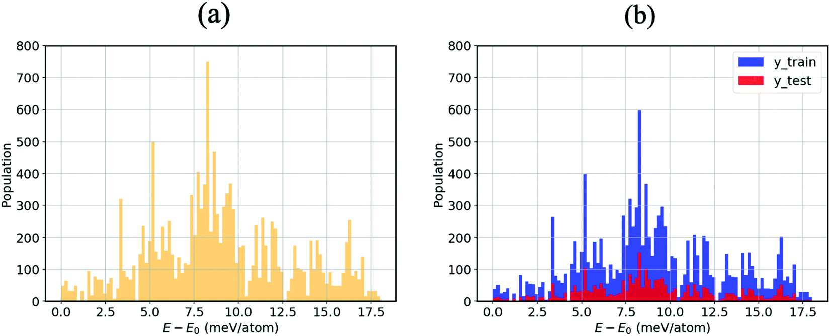Fig. 2 (a) Energy population distribution (meV per atom) corresponding to the various MA orientations split into 100 bins. (b) Training set (80% of the total samples) and test set (the other 20%) of MABiSeI used in our proposed neural network.

Fig. 3 (a) Four-dimensional plot of E − E₀ (meV) with respect to angles ϕ, θ, and ψ. (b) Three-dimensional and contour plots of E − E₀ with ϕ = 45°. See the main text for a description.

To preserve the orthogonality of the four-dimensional axes, a series of cross-sections visualising the three-dimensional energy landscapes are clearly delineated. The topographic features of the energetics accounting for the MA cation orientations are illustrated, as an example, by the ΔE(ϕ = 45°, θ, ψ) slice, shown in Fig. 3(b). The landscape, defining how the organic molecule jiggles within the inorganic framework, obviously comprises four repeating patterns of a single mountain surrounded by a couple of deep pits and a little cup on the left (see also the contour plot). Being amongst a large set of highest peaks with ΔE = 17.9 meV per atom, these four energy barriers—slightly smaller than those of FAPbI₃ (with the highest peak of 24.7 meV per atom)⁹ and MAPbI₃ (18.6 meV/MA-cation)³³ —roughly imply that a thermal excitation energy of ∼208 K is required to flip the MA cation according to a given path in the configurational landscape, provided that ΔE ∼ k_BT, whereas the pits indicate the energetically preferred orientations due to their lowest possible total energy. More importantly, further along the θ-axis from its origin in Fig. 3(a), on the left stands a couple of the highest mountains, consistent with the cross-section shown in Fig. S1(b) (ESI†). By the same token, similar characteristics can be seen along the ψ-axis (see also Fig. S1(c), ESI†). In accordance with these two 2D landscapes with a period of 180°, when the MA cation flips along the C–N shaft for its period, the environment remains unchanged. It is worth mentioning that the 3D landscapes are geometrically reducible so that the equivalence sets can be observed once only: namely, ΔE(ϕ, θ, ψ) = ΔE(ϕ, 360° − θ, ψ) in the θ-fixed scheme and ΔE(ϕ, θ, ψ) = ΔE(ϕ + 180°, θ, ψ) in the ϕ-fixed scheme.

However, if one considers the relationship between ΔE and ϕ, a supposedly Gaussian barrier with a period of 90° (see Fig. S2, ESI†) emerges, similar to previous works,^9,34 with a highest barrier of 9.6 meV per atom, which is attributable to the fact that the dipole merely azimuthally turns away from I2 to I1, and vice versa. The (ϕ + n·90°, θ, 0°) configurations (with n = 1, 2, 3, and 4) blatantly resemble a set of preferred orientations of local minima (ΔE = 3–4 meV per atom) separated by arrays of saddle reefs, and the H atoms thereby prefer pointing towards the I atom. Also, the ψ-fixed schemes are reducible according to the relationship ΔE(ϕ, θ, ψ) = ΔE(ϕ, θ, ψ + 180°). That being said, the bivariate or pairwise correlations between each Euler angle and ΔE, expressed by the Pearson's correlation coefficient (ρ),³⁵ are far from unity (ranging from −0.013 to 0.044), roughly suggesting no linear correlation. The remaining 3D landscapes are reported in Fig. S2–S12 (ESI†).

3.2 Neural network

The building blocks of neural networks are single artificial neurons.³⁶ A single neuron can be thought of as a map taking several inputs x₁, x₂,…, x_n and providing an output , which is passed through an activation function A, where the weights w_i ∈ R and the bias b ∈ R are tuned during training. Consequently, a neural network is created by aggregating neurons into layers, which might perform different transformations on their inputs, and finally the outputs accord to the activation of the last neuron(s) in the last layer,²⁵ as schematically shown in Fig. 4. Furthermore, the universality of neural networks, implying they can be exploited to approximate any continuous function to an arbitrary accuracy given appropriate weights,³⁷ piques our interest in dealing with complicated trends regarding our high-dimensional energy landscape for the rigid-body rotations of the MA cation.

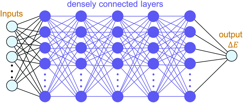Fig. 4 Topology of our neural network model: an input layer consisting of ten features including three Euler angles and selected bond-lengths, i.e. C1–Bi1, C1–Se1, C1–I1, C1–I2, H1–Bi1, H2–Bi1, and H3–Bi1, which feeds five densely connected hidden layers (of 500 neurons each), the last of which is connected to an output node outputting ΔE ≡ E − E₀.

With the aim of capturing the complex trends and correlations of high-dimensional data within energy landscapes, the artificial neural network (ANN), being the current in vogue statistical tool based on deep learning, is designed using the Keras frontend on top of the Tensorflow machine learning library.^38,39 The aim is then achieved by inputting, for example, the angles of rotations (ϕ, θ, and ψ) as input features/descriptors, and outputting ΔE by means of regression. Generally, feature augmentation is also crucial for reducing the probability of losing important information which might improve the predictions.⁴⁰ Thus, pairwise bond lengths are included as descriptors in addition to the Euler angles. Fig. S14 (ESI†) presents a set of seven pairwise relationships expressed by parallel axes, intensively discussed by Wegman et al.⁴¹Fig. 4 illustrates pictorially the best tweaked ANN regressor architecture comprising an input layer, feeding three Euler angles together with C–Bi, C–Se, C–I1, C–I2, H1–Bi, H2–Bi, and H3–Bi bond-lengths, which is accompanied by five fully connected hidden layers with 500 neurons each, and an output layer which takes the output of the previous fully connected layer as an input and calculates the value of ΔE via a linear activation function. To train our model, 13 824 samples in our dataset are randomly sorted, as represented in Fig. 2(b), where 80% are set as the training set (11 059 samples) and 20% (2765 samples) as the test set. The root mean square error (RMSE) between the predicted and the DFT-calculated values is utilised as the cost function, which is minimised during training using the Adam stochastic optimiser.⁴² To improve the training behaviour, the dataset is normalised by subtracting the mean of each feature from each value and dividing by the feature range so that all values are within the range of 0 and 1. The training process is repeated 10 times so that the optimised values are in good agreement with a maximum 5% error.

As a result, Fig. 5(a) evidences the improvement in our ANN with an increase in the number of hidden layers. The RMSEs corresponding to both the training set (blue) and test set (red) taper off at 5 hidden layers, specifically when each layer consists of 500 neurons, with which the model shows no sign of overfitting (a modelling error that occurs when a relationship/function is too closely or exact a fit to a particular set of data), i.e., RMSE = 0.39 ± 0.03 meV per atom for the test set, while they gradually increase when the number of layers grows over 6 hidden layers and begin to overfit at 9 hidden layers onwards. Likewise, 500 neurons per layer for each of the five hidden layers are confirmed to have the relatively lowest error, as reported in Fig. 5(b). This confirms that the smallest error occurs at 500 neurons for each hidden layer. Fig. 5(c) reports the results obtained from our optimised ANN regressor with the obtained RMSEs of 0.24 meV per atom for the training set and 0.37 meV per atom for the test set. It is clear that our data-driven framework provides a reliable estimation of the DFT calculations using around 10⁴ training data, together with ten properties of inorganic crystals, as the input by designing and systematically optimising a neural network regressor to output ΔE close to the DFT obtained values.

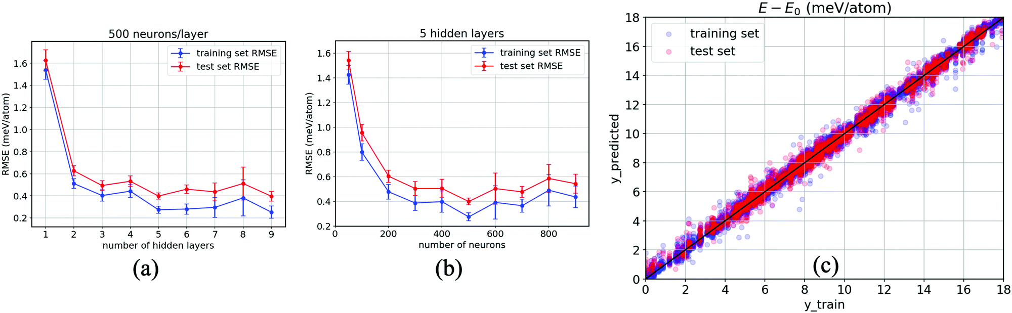Fig. 5 Variation of the root mean square error (RMSE) of the training set (blue) and test set (red) with respect to the number of hidden layers (a), and to the number of neurons for each hidden layer (b). Representative plots for the prediction of the optimised neural network with 80% of the data for training and 20% for testing, with training set RMSE = 0.24 meV and test set RMSE = 0.37 meV (c).

It is worth mentioning that our assumption, keeping the inorganic framework unchanged, is based on a simple model in which the other chemical and physical factors in this hybrid material are not taken into consideration, especially when designing the neural network. It, however, provides a good starting point for further study, where other factors such as the distortion of the inorganic cages, as well as the long-range molecular interaction between the MA cation and its counterparts embedded in the neighbouring unit cells, should be incorporated as inputs for the neural network. As such, this will require a supercell in which the MA cations are arranged differently according to the Euler angles applied.

4 Conclusion

In summary, the total energy profiles of the cubic MABiSeI perovskite were evaluated using DFT with the inclusions of vdW interactions and the SOC effect. By applying Euler angles to the MA cation, the dynamic behaviours of the MA cations are described through multidimensional total energy landscapes. Slices of the three-dimensional energy landscapes reveal local and global minima for the organic cation's preferred orientations as well as the highest barriers of 17.9 meV per atom, equivalent to 208 K, that protrude from the plateau of the average height of 9 meV per atom. We also developed an artificial neural network to accurately predict the total energies, with the resulting RMSE of 0.37 meV per atom for the test set, by inputting the Euler angles and seven sets of bond lengths as descriptors. We propose a new approach for designing a set of analyses and developing a high-fidelity deep learning based tool which can necessarily disregard the DFT calculations, and in turn makes promising predictions of the total energy for the lead-free CH₃NH₃BiSeI₂ perovskite. This approach might possibly be useful in predicting the thermodynamic properties of the molecular rotations of similar materials at large scales, provided that the intermolecular interactions are known, instead of relying only on DFT calculations which are undoubtedly computationally demanding.

Conflicts of interest

There are no conflicts to declare.

Acknowledgements

This work was partially supported by the Sci Super-IV research grant, Faculty of Science, Chulalongkorn University. This research was funded by Chulalongkorn University; Grant for Research, and the Ratchadapisek Somphot Fund for Postdoctoral Fellowships, Chulalongkorn University. Also, we gratefully acknowledge the Thailand Center of Excellence in Physics (ThEP), as well as the strong support from the Science Achievement Scholarship of Thailand (SAST). We also thank Mr Vichayanun Wachirapusitanand for his additional techniques in the Matplotlib library. A. E. gratefully acknowledges the financial support from the Ratchadaphiseksomphot Endowment Fund, Chulalongkorn University, the Grants for the Development of New Faculty Staff, and from the Sci-Super VI fund, Faculty of Science, Chulalongkorn University. T. B. acknowledges National Research Council of Thailand (NRCT): (NRCT5-RSA63001-04). B. A. acknowledges financial support from the Swedish Government Strategic Research Area in Materials Science on Functional Materials at Linköping University, Faculty Grant SFOMatLiU No. 2009 00971, as well as support from the Swedish Foundation for Strategic Research through the Future Research Leaders 6 program, FFL 15-0290, from the Swedish Research Council (VR) through the grant 2019-05403, and the Knut and Alice Wallenberg Foundation (Wallenberg Scholar Grant No. KAW-2018.0194). All of the density functional theory calculations were carried out using supercomputer resources provided by the Swedish National Infrastructure for Computing (SNIC) performed at the National Supercomputer Centre (NSC).

References

1. H. Zhou, Q. Chen, G. Li, S. Luo, T.-B. Song, H.-S. Duan, Z. Hong, J. You, Y. Liu and Y. Yang, Science, 2014, 345, 542–546.
2. M. A. Green, A. Ho-Baillie and H. J. Snaith, Nat. Photonics, 2014, 8, 506.
3. T. M. Brenner, D. A. Egger, L. Kronik, G. Hodes and D. Cahen, Nat. Rev. Mater., 2016, 1, 1–16.
4. S. D. Stranks, G. E. Eperon, G. Grancini, C. Menelaou, M. J. Alcocer, T. Leijtens, L. M. Herz, A. Petrozza and H. J. Snaith, Science, 2013, 342, 341–344.
5. J. M. Frost, K. T. Butler, F. Brivio, C. H. Hendon, M. Van Schilfgaarde and A. Walsh, Nano Lett., 2014, 14, 2584–2590.
6. C. C. Stoumpos, C. D. Malliakas and M. G. Kanatzidis, Inorg. Chem., 2013, 52, 9019–9038.
7. M. T. Weller, O. J. Weber, P. F. Henry, A. M. Di Pumpo and T. C. Hansen, Chem. Commun., 2015, 51, 4180–4183.
8. R. Klinkla, V. Sakulsupich, T. Pakornchote, U. Pinsook and T. Bovornratanaraks, Sci. Rep., 2018, 8, 1–9.
9. W. Sukmas, U. Pinsook, P. Tsuppayakorn-aek, T. Pakornchote, A. Sukserm and T. Bovornratanaraks, J. Phys. Chem. C, 2019, 123, 16508–16515.
10. J. S. Bechtel, R. Seshadri and A. Van der Ven, J. Phys. Chem. C, 2016, 120, 12403–12410.
11. D. H. Cao, C. C. Stoumpos, O. K. Farha, J. T. Hupp and M. G. Kanatzidis, J. Am. Chem. Soc., 2015, 137, 7843–7850.
12. A. H. Slavney, R. W. Smaha, I. C. Smith, A. Jaffe, D. Umeyama and H. I. Karunadasa, Inorg. Chem., 2017, 56, 46–55.
13. F. Hao, C. C. Stoumpos, D. H. Cao, R. P. Chang and M. G. Kanatzidis, Nat. Photonics, 2014, 8, 489.
14. D. Sabba, H. K. Mulmudi, R. R. Prabhakar, T. Krishnamoorthy, T. Baikie, P. P. Boix, S. Mhaisalkar and N. Mathews, J. Phys. Chem. C, 2015, 119, 1763–1767.
15. Y.-Y. Sun, M. L. Agiorgousis, P. Zhang and S. Zhang, Nano Lett., 2015, 15, 581–585.
16. K. Momma and F. Izumi, J. Appl. Crystallogr., 2011, 44, 1272–1276.
17. I. Repins, M. A. Contreras, B. Egaas, C. DeHart, J. Scharf, C. L. Perkins, B. To and R. Noufi, Prog. Photovoltaics, 2008, 16, 235–239.
18. C. Wang, S. Chen, J.-H. Yang, L. Lang, H.-J. Xiang, X.-G. Gong, A. Walsh and S.-H. Wei, Chem. Mater., 2014, 26, 3411–3417.
19. I. Grinberg, D. V. West, M. Torres, G. Gou, D. M. Stein, L. Wu, G. Chen, E. M. Gallo, A. R. Akbashev and P. K. Davies, et al. , Nature, 2013, 503, 509–512.
20. S. Balaz, S. H. Porter, P. M. Woodward and L. J. Brillson, Chem. Mater., 2013, 25, 3337–3343.
21. L. M. Schoop, L. Muchler, C. Felser and R. J. Cava, Inorg. Chem., 2013, 52, 5479–5483.
22. Y.-Y. Sun, J. Shi, J. Lian, W. Gao, M. L. Agiorgousis, P. Zhang and S. Zhang, Nanoscale, 2016, 8, 6284–6289.
23. W. Shockley and H. J. Queisser, J. Appl. Phys., 1961, 32, 510–519.
24. P. Hohenberg and W. Kohn, Phys. Rev., 1964, 136, B864.
25. I. Goodfellow, Y. Bengio, A. Courville and Y. Bengio, Deep learning, vol. 1, 2016.
26. P. E. Blöchl, Phys. Rev. B: Condens. Matter Mater. Phys., 1994, 50, 17953.
27. G. Kresse and J. Furthmüller, Phys. Rev. B: Condens. Matter Mater. Phys., 1996, 54, 11169.
28. J. P. Perdew, K. Burke and M. Ernzerhof, Phys. Rev. Lett., 1996, 77, 3865.
29. D. Hobbs, G. Kresse and J. Hafner, Phys. Rev. B: Condens. Matter Mater. Phys., 2000, 62, 11556.
30. S. Ehrlich, J. Moellmann, W. Reckien, T. Bredow and S. Grimme, ChemPhysChem, 2011, 12, 3414–3420.
31. H. J. Monkhorst and J. D. Pack, Phys. Rev. B: Solid State, 1976, 13, 5188.
32. J. D. Hunter, Comput. Sci. Eng., 2007, 9, 90–95.
33. W. Sukmas, V. Sakulsupich, P. Tsuppayakorn-Aek, U. Pinsook, T. Pakornchote, R. Klinkla and T. Bovornratanaraks, Sci. Rep., 2020, 10, 1–8.
34. D. H. Fabini, T. A. Siaw, C. C. Stoumpos, G. Laurita, D. Olds, K. Page, J. G. Hu, M. G. Kanatzidis, S. Han and R. Seshadri, J. Am. Chem. Soc., 2017, 139, 16875–16884.
35. K. Pearson, Proc. R. Soc. London, 1895, 58, 240–242.
36. H. Wang and B. Raj, arXiv preprint arXiv:1702.07800, 2017.
37. K. Hornik, Neural Networks, 1991, 4, 251–257.
38. F. Chollet et al. , https://keras.io/k, 2015, 7, T1.
39. M. Abadi, A. Agarwal, P. Barham, E. Brevdo, Z. Chen, C. Citro, G. S. Corrado, A. Davis, J. Dean and M. Devinet al., arXiv preprint arXiv:1603.04467, 2015.
40. W. A. Saidi, W. Shadid and I. E. Castelli, npj Comput. Mater., 2020, 6, 1–7.
41. E. J. Wegman, J. Am. Stat. Assoc., 1990, 85, 664–675.
42. D. P. Kingma and J. Ba, arXiv preprint arXiv:1412.6980, 2014.

---

Footnote

† Electronic supplementary information (ESI) available. See DOI: 10.1039/d1ma00076d

---