
 Open Access Article
 This Open Access Article is licensed under a
 Creative Commons Attribution 3.0 Unported Licence
Simulations of valence excited states in coordination complexes reached through hard X-ray scattering†
Erik
Källman
a,
Meiyuan
Guo
 a,
Mickaël G.
Delcey
a,
Drew A.
Meyer
b,
Kelly J.
Gaffney
c,
Roland
Lindh
de and
Marcus
Lundberg
*a
a,
Mickaël G.
Delcey
a,
Drew A.
Meyer
b,
Kelly J.
Gaffney
c,
Roland
Lindh
de and
Marcus
Lundberg
*a
aDepartment of Chemistry – Ångström Laboratory, Uppsala University, S-75120 Uppsala, Sweden. E-mail: marcus.lundberg@kemi.uu.se
bDepartment of Chemistry, Case Western Reserve University, Cleveland, OH 44106, USA
cPULSE Institute, SLAC National Accelerator Laboratory, Stanford University, Menlo Park, CA 94025, USA
dDepartment of Chemistry – BMC, Organic Chemistry, Uppsala University, S-75105 Uppsala, Sweden
eUppsala Center for Computational Chemistry (UC3), Uppsala University, P.O. Box 596, SE-751 24 Uppsala, Sweden
First published on 26th March 2020
Abstract
Hard X-ray spectroscopy selectively probes metal sites in complex environments. Resonant inelastic X-ray scattering (RIXS) makes it is possible to directly study metal–ligand interactions through local valence excitations. Here multiconfigurational wavefunction simulations are used to model valence K pre-edge RIXS for three metal-hexacyanide complexes by coupling the electric dipole-forbidden excitations with dipole-allowed valence-to-core emission. Comparisons between experimental and simulated spectra makes it possible to evaluate the simulation accuracy and establish a best-modeling practice. The calculations give correct descriptions of all LMCT excitations in the spectra, although energies and intensities are sensitive to the description of dynamical electron correlation. The consistent treatment of all complexes shows that simulations can rationalize spectral features. The dispersion in the manganese(III) spectrum comes from unresolved multiple resonances rather than fluorescence, and the splitting is mainly caused by differences in spatial orientation between holes and electrons. The simulations predict spectral features that cannot be resolved in current experimental data sets and the potential for observing d–d excitations is also explored. The latter can be of relevance for non-centrosymmetric systems with more intense K pre-edges. These ab initio simulations can be used to both design and interpret high-resolution X-ray scattering experiments.
1 Introduction
Transition metal complexes can facilitate a wide variety of different processes. Their versatility comes from the potential to tune the energy of close-lying valence levels through metal–ligand interactions. Electron spectroscopy in the UV-Vis region probes these interactions through excitations between filled and empty valence orbitals. However, in complex systems with many different absorbers, the signals from the metal center can be easily obscured. In addition, the large number of different excitations can make it difficult to assign transitions, e.g., to separate between overlapping ligand-to-metal charge-transfer (LMCT) and metal-to-ligand charge-transfer (MLCT) transitions.X-ray spectroscopy is an element specific technique where the core hole acts as localized probe of the electronic structure around the metal. Valence excitations can be studied through the use of resonant inelastic X-ray scattering (RIXS).1,2 In this two-photon process, absorption of an incident photon is followed by emission of a scattered photon. Their energy difference is equal to the energy required to reach the excited state.3–8 For first-row transition metals, soft X-ray L-edge RIXS (2p → 3d → 2p) directly probes the metal 3d orbitals. That leads to a relative enhancement of the metal-centered excitations and a clear separation of MLCT and LMCT excitations along the incident energy axis.2 The lifetime broadening in the emission energy is dictated by the final state lifetime, which for a valence excited state can be quite small. The rich spectral information has been used to extract detailed electronic structure information and to follow ultrafast excited-state dynamics.9–12
A challenge with soft X-ray RIXS is the significant background absorption associated with the generation of photoelectrons from lighter elements, which also can lead to sample damage even at low X-ray doses.13,14 For first-row transition metals excitations in the metal K edge, which involves the metal 1s orbital, instead requires photon energies of thousands of eV. These hard X-rays are only weakly absorbed by the environment, which reduces background absorption and the propensity for photodamage. Hard X-ray RIXS has been extensively used to probe both metal-centered and metal–ligand excitations.3,15–26 In direct RIXS, excitation is made directly into the metal K pre-edge (1s → 3d),21,23–25,27 which can in itself be used to understand both geometric and 3d-orbital electronic structure.28 The experiment is challenging due to relatively low photon counts. The 1s → 3d excitation is electric-dipole forbidden in centrosymmetric systems and to directly access valence excited states, this should be coupled to a valence →1s (Kβ2,5) emission process, see Fig. 1.23 For enzymes and coordination complexes, which can both have low metal concentrations and be sensitive to X-ray induced damage even with hard X-rays, it is more common to use the intense Kα or Kβ1,3 emission channels.29–32 However, with upgraded synchrotron lightsources offering increased photon flux and more efficient detectors, valence K-edge RIXS can become an attractive spectroscopic probe for a wider range of systems.
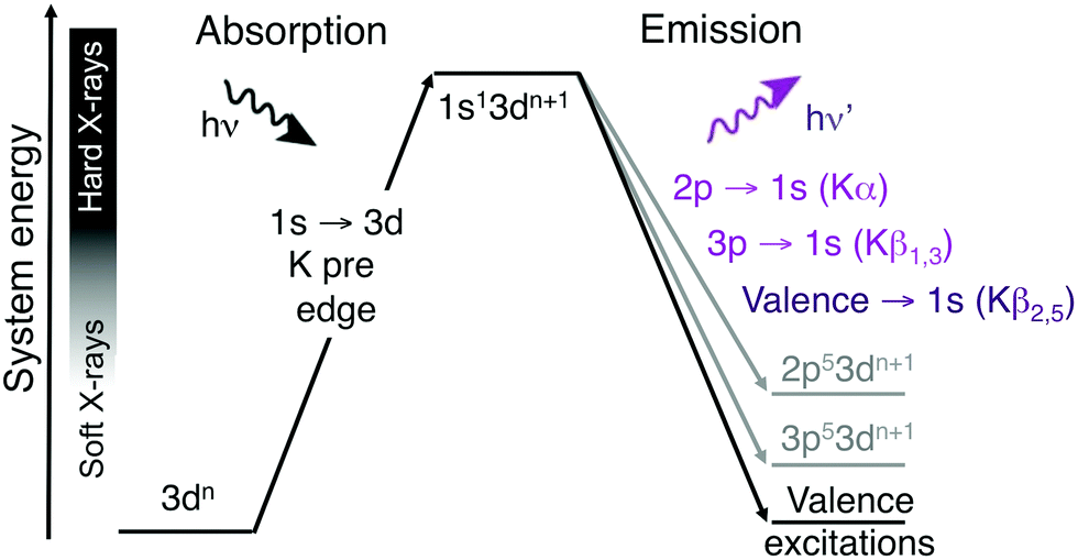 | ||
| Fig. 1 Two-step schematic of the hard X-ray direct RIXS process. The vertical axis shows the total energy of the electron configuration (not to scale). | ||
An efficient design of new valence K-edge RIXS experiments requires predictions of the expected information content. Previous models include crystal-field multiplet, exact diagonalization, multiple scattering, and charge-transfer multiplet (CTM) models.21,33–35 Here the aim is to use an ab initio molecular orbital model that can directly link spectra to electronic structure of coordination complexes. This will be achieved through multiconfigurational simulations based on the restricted active space (RAS) formalism.36,37 This model can explicitly include the large number of molecular orbitals involved in the valence RIXS process, and at the same time correctly describe the wavefunctions arising from the coupling of multiple open shells. It has previously been used to simulate X-ray processes of both first-row transition metals and heavy elements.9,38–43 We recently implemented a complete second-order expansion of the wave-vector,44 required to model dipole-forbidden K pre-edges, and applied it to both X-ray absorption spectroscopy (XAS) and Kα RIXS.45–47
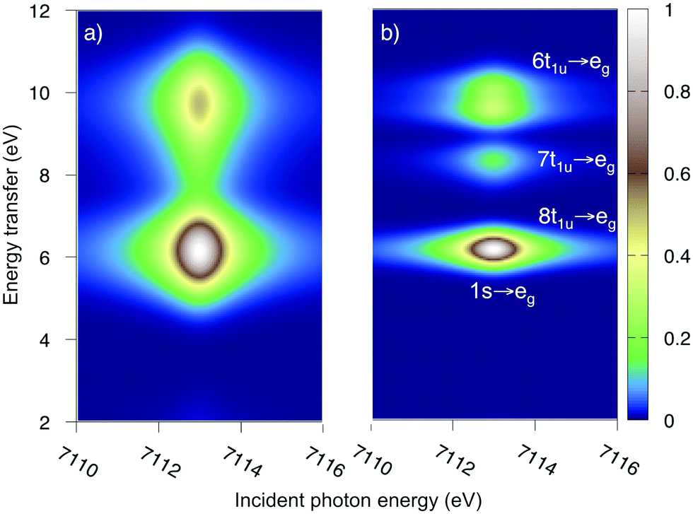
The multiconfigurational simulations of the RIXS process will be made for a series of metal hexacyanide complexes. Metal hexacyanides have been widely used as model systems for new experimental and theoretical X-ray techniques.11,12,23,41,48–54 Valence K-edge RIXS spectra have been collected for three systems with different d-electron counts: [FeII(CN)6]4− (ferrocyanide), [FeIII(CN)6]3− (ferricyanide), and [MnIII(CN)6]3− (manganicyanide).23,27 The spectrum for ferrocyanide is shown in Fig. 2. The intensity is plotted as a function of the incident photon energy (Ω) and the energy transfer (Ω–ω). The y-axis thus corresponds to the energy of the final states reached in the RIXS process, and is directly comparable to valence-excitation energies. The spectrum has one pre-edge resonance with at least three emission resonances, followed by the rising edge. The other two complexes have multiple pre-edge resonances, which leads to a large number of different valence-excited states, separated either by incident or emission energy in the RIXS planes. These rich data sets can be used to rigorously test the performance of different modeling protocols and to establish the accuracy of the current RAS approach.
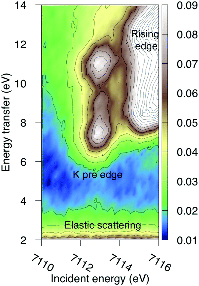 | ||
| Fig. 2 Experimental RIXS plane of [FeII(CN)6]4− (ferrocyanide). Data from ref. 27. The absolute intensity scale is arbitrary. | ||
2 Computational details
All RAS calculations have been performed using OpenMolcas.55 The three modeled complexes, iron(II), iron(III), and manganese(III), represent 3d6, 3d5, and 3d4 electron configurations. The CN− ligands create a strong ligand field and all d-electrons are therefore in the three t2g orbitals. This leads to singlet (S = 0), doublet (S = 0.5), and triplet (S = 1) ground states respectively. Note that symmetry labels from the well-known Oh point group will be used throughout because all complexes either belong to, or are close to, this group. In practice, calculations are performed using the Abelian point group D2h.A 7-orbital RAS2 space (RAS2-A) has been designed including the five metal-dominated t2g and eg orbitals as well as two ligand-dominated σ orbitals of eg symmetry, see Fig. 3. Isodensity plots of these orbitals are shown in ESI† Fig. SI-1. Calculations have also been performed with a 10-orbital RAS2 space, called RAS2-B, which in addition includes three empty 4d-type t2g orbitals for double-shell correlation.56 For calculations with a large number of excited states these orbitals instead become ligand-dominated pi* orbitals,40 as discussed in more detail below. To model the K pre-edge excitations, the metal 1s orbital is placed in the RAS3 space allowing up to two electrons. In addition, four sets of filled ligand-dominated orbitals were included in the RAS1 space, allowing a single hole, see Fig. 3. Only molecular orbitals in the t1u irreducible representation gives dipole allowed transitions to 1s, but in D2h symmetry both t1u and t2u transform to b1u,2u,3u. Therefore, the 1t2u molecular orbitals were added to the dipole-allowed 6t1u, 7t1u, and 8t1u orbitals, see isodensity plots in Fig. 4. These four sets roughly correspond to the CN− molecular 5σ (t1u), 1π (t1u + t2u), and 4σ (t1u) orbitals. For details about the t1u and t2u orbital diagram, see Fig. SI-2 (ESI†).
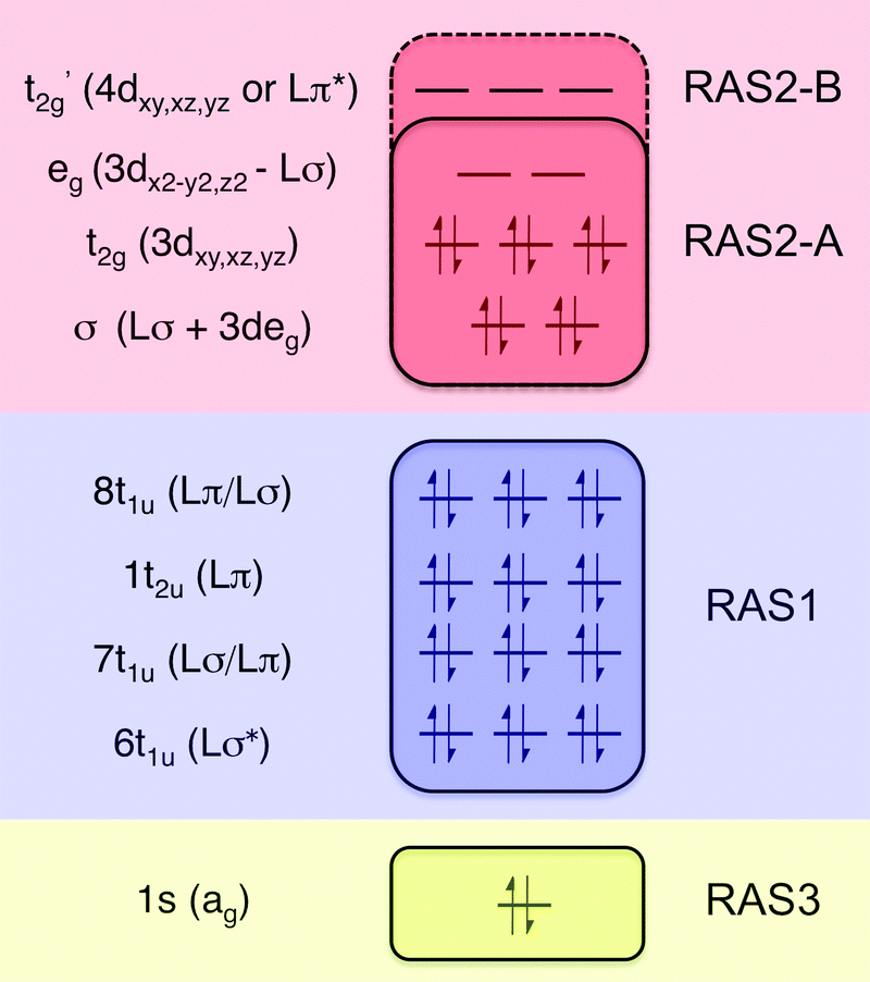 | ||
| Fig. 3 Active-space selection for the valence K pre-edge RIXS process. The electron configuration represents the ferrocyanide ground state. | ||
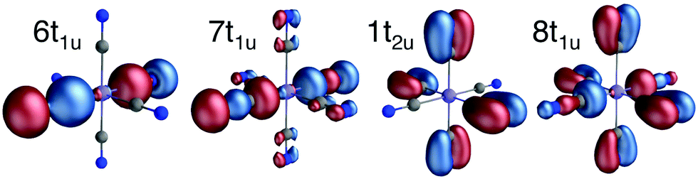 | ||
| Fig. 4 Isodensity representations of the four filled ligand-dominated orbitals in the RAS1 space. Orbital pictures are from the b1u representation in the ferrocyanide ground state. | ||
Orbital optimizations were performed using the state-average (SA) RAS self-consistent field (SCF) method with the ANO-RCC-VTZP basis set,57,58 in the resolution of identity approximation with atomic-compact Cholesky decomposition-derived auxiliary basis.59,60 Final energies and wavefunctions were calculated using second-order perturbation (PT2) theory61 in three different versions: state-specific (SS), multi-state (MS),62 and extended multi-state (XMS).63 The multi-state method couples the different states through an effective Hamiltonian which depends on the individual Fock matrices of the states under consideration. By contrast, the extended multi-state method uses the state-average density to compute the Fock matrix, which allows for computation of the off-diagonal elements between all states, but gives worse state energies, especially as the number of states increases. Unless otherwise specified, results are from MS-RASPT2 calculations including all SA-RASSCF states. An imaginary shift of 0.3 Hartree and the default ionization-potential electron-affinity (IPEA) shift of 0.25 Hartree has been used.64,65 Scalar relativistic effects have been included by using a second-order Douglas–Kroll–Hess Hamiltonian and spin–orbit coupling through the RAS state-interaction (RASSI) approach.66–69
Geometry optimizations were performed using the ten-orbital RAS2-B space, see Fig. 3. Optimized bond distances of the three complexes are given in Table SI-1 (ESI†). FeII has a symmetric 1A1g ground state. MnIII and FeIII, show small Jahn–Teller (JT) distortions but remain centrosymmetric. The triple orbital near-degeneracy, coupled to doublet and triplet spin multiplicity gives six and nine low-lying spin–orbit states, see Fig. SI-3 (ESI†). Compared to the spin–orbit coupling, the splitting from the JT distortion is small and not expected to have a significant effect on the spectra.51
Calculations are performed separately for each of the eight irreducible representations in the D2h point group, and with separate optimizations in initial, intermediate and final states. Up to 200 final states were used to test the convergence of the RIXS spectra. The calculations were made possible by a new stable and efficient algorithm for CI calculations with a large number of states, which is now the default algorithm in OpenMolcas.70 For detailed information about the number of states in different calculations, see Tables SI-2 and SI-3 (ESI†). As all complexes are centrosymmetric, the LMCT states are simply the lowest states with ungerade symmetry. To reach the high-energy core-excited states, a projection technique is used to remove all configurations with doubly-occupied core orbitals in the intermediate state (HEXS keyword).45,70 To avoid orbital rotation, i.e., that the hole appears in a higher-lying orbital, the 1s orbital was not re-optimized in the core-excited states. As the spin–orbit coupling remains relatively weak during the RIXS process, only intermediate and final states of the same spin multiplicity as the initial state have been included.
Molecular crystals are held together by non-covalent interactions, leading to narrow band widths. Band structure has therefore been neglected. To calculate spectra, the surrounding has been modeled using a PCM environment with a high dielectric constant (ε = 80). This effectively leads to charge compensation for these highly negative model complexes. Considering the femtosecond time scale of the scattering process, both intermediate and final states have been calculated with non-equilibrium solvation taken from the initial state. The short timescale also means that structural evolution in the core-excited state can be neglected.
Transition matrix elements up to a full second-order expansion of the wave vector have been calculated using RASSI.46 In principle, the plane-wave form of the wave vector could also be used,71–74 but as that operator depends on the transition energy, the cost of evaluating a scattering processes that includes tens of thousands of individual transitions becomes too high. Here K pre-edge XAS spectra have been simulated using the exact operator for comparison with the multipole expansion. For RASPT2 calculations the second-order expansion usually performs well in combination with a reasonably large basis set like ANO-RCC-VTZP.47 A more detailed analysis of individual transitions indicate that true convergence can require a very high order of the expansion, but this has smaller consequences for the calculated intensities because the redistribution occurs among close-lying transitions.75 The K pre-edge spectra were calculated using the 10-orbital RAS2-B space following the previously published protocol.45 The same active space is then used to calculate d–d RIXS spectra, which only includes transitions between 1s and the gerade valence orbitals. LMCT RIXS spectra are instead calculated using the 7-orbital RAS2 space. The main difference is the lack of correlation of the t2g orbitals. Therefore, the relative energy of the states reached through 1s → t2g transitions have been corrected to match those of the 10-orbital spaces, see the Results section below.
The RIXS spectra can be calculated from the Kramers-Heisenberg formula:
 | (1) |
![[T with combining circumflex]](https://www.rsc.org/images/entities/i_char_0054_0302.gif) a and e are transition operators for the absorption and emission processes respectively. K(Γ) depends on the resonance energy and the lifetime broadening Γ of each state. We use calculated oscillator strengths to generate RIXS spectra, which is equivalent to neglecting interference effects:
a and e are transition operators for the absorption and emission processes respectively. K(Γ) depends on the resonance energy and the lifetime broadening Γ of each state. We use calculated oscillator strengths to generate RIXS spectra, which is equivalent to neglecting interference effects: | (2) |
Contributions from different initial states have been included according to their Boltzmann weight at room temperature, see Fig. SI-3 (ESI†).
Comparisons with experiment are done using data from ref. 23 and 27. Calculated spectra were broadened using a Lorentzian lifetime broadening of 1.25 eV (Fe) and 1.16 eV (Mn) full-width half-maximum (FWHM) in the incident energy direction, widths that have been obtained from semi-empirical calculations.76 The spectra are then convoluted with experimental Gaussian broadenings of 0.2 eV FWHM in the incident energy direction and 1.5 eV FWHM in the energy transfer direction.23 Hypothetical high-resolution spectra have been generated using a 0.6 eV broadening in the energy transfer direction. Incident energies have been globally shifted to match the first pre-edge peaks of the experimental spectra, see Table SI-4 (ESI†). As described in the Results section below, the position of the first energy transfer resonance has been calculated using an equivalent number of initial and final states in the SA-RASSCF calculations. No further corrections have been made in the energy-transfer direction. K pre-edge intensities are multiplied by 2881 to match experimental K-edge XAS spectra normalized to unity at the edge-jump.45 Calculated RIXS intensities are scaled to unity at the maximum.
3 Results and discussion
Among the three model complexes, the RIXS process of iron(II) hexacyanide is the most straightforward. Low-spin iron(II) has a closed-shell singlet ground state, and the K pre-edge consists of a single 1s → eg peak.28 The iron(II) spectrum will therefore be used for an in-depth analysis of model performance. This will be followed by results for the other two complexes, which makes it possible to compare and contrast the results for different electronic structures.3.1 Iron(II) hexacyanide RIXS spectrum
As mentioned above, the experimental ferrocyanide spectrum has one pre-edge resonance at 7113.0 eV with three energy-transfer resonances, see Fig. 2. These resonances can be tentatively assigned to come from emission from the 8t1u, 7t1u, and 6t1u ligand-dominated orbitals, which results in LMCT final states. In UV-Vis there are strong charge-transfer excitations at 5.7 and 6.2 eV. These do not appear in the experimental LMCT RIXS spectrum where the first resonance is at 7.4 eV. These UV-Vis resonances can therefore be assigned to MLCT excitations, which is in line with previous analysis.77The K pre-edge spectrum of ferrocyanide has been previously simulated with RAS.45 The 1s → eg excitation leads to a doubly degenerate state with one unpaired electron in two eg orbitals. The modeled MS-RASPT2 RIXS spectrum, with two different experimental broadenings, is shown in Fig. 5. It also has three resonances separated by approximately 2 eV along the energy transfer axis, in good agreement with experiment.27 The second peak is not visible when plotting the results with the experimental resolution (Fig. 5a), but becomes clear with higher resolution (Fig. 5b). As the simulations focus on pre-edge transitions, the rising edge of the experimental spectrum is not included.
 | ||
| Fig. 5 Iron K pre-edge RIXS spectra of the ferrocyanide from multi-state RASPT2 calculations with 40 ungerade valence states. (a) Experimental resolution (1.5 eV FWHM in the energy transfer direction). (b) Higher resolution (0.6 eV FWHM). | ||
Direct comparisons of energies and relative intensities between experimental and modeled spectra are given in Table 1. The computational model is qualitatively correct, but has some quantitative errors. Peak energies are underestimated by around 1 eV. The 3.6 eV splitting between low and high-energy peaks is better described with an error of 0.2 eV, although the relative position of the middle peak is too high. Regarding intensities, the distinct experimental pattern with lower intensity of the middle peak compared to the other two is reproduced. However, the intensity of the first peak is overestimated while the second peak is underestimated.
| System | Resonance | Data | Incident (eV) | Transfer (eV) | Intensitya | ||||
|---|---|---|---|---|---|---|---|---|---|
| a Theoretical intensities are extracted from spectra plotted with experimental resolution using peak positions from high-resolution spectra. b From ref. 27. c Aligned to experimental data. d Extracted from experimental data in ref. 23. | |||||||||
| Fe(II) | eg | Exp.b | 7113.0 | 7.4 | 9.1 | 11.1 | 1.00 | 0.63 | 0.99 |
| Theory | 7113.0c | 6.2 | 8.3 | 9.7 | 1.00 | 0.22 | 0.50 | ||
| Fe(III) | t2g | Exp.b | 7110.2 | 3.2 | 4.9 | 7.2 | 0.21 | 0.08 | 0.17 |
| Theory | 7110.2c | 3.1 | 5.2 | 6.9 | 0.42 | 0.03 | 0.30 | ||
| eg | Exp. | 7113.2 | 6.4 | 8.0 | 10.1 | 0.70 | 0.32 | 1.00 | |
| Theory | 7113.2 | 6.2 | 7.8 | 9.5 | 1.00 | 0.27 | 0.72 | ||
| Mn(III) | t2g | Exp.d | 6539.1 | 4.0 | 5.6 | 7.6 | 0.97 | 0.58 | 0.83 |
| Theory | 6539.1c | 4.2 | 6.1 | 7.8 | 1.00 | 0.20 | 0.44 | ||
| eg | Exp. | 6541.4 | 6.7 | 7.8 | 9.8 | 0.90 | 0.78 | 1.00 | |
| Theory | 6540.9 | 6.6 | 8.1 | 9.0 | 0.91 | 0.36 | 0.42 | ||
The high-resolution spectrum in Fig. 5b shows structure in the emission resonances, most visibly in the high-energy peak. This is consistent with previous analysis of the K pre-edge RIXS process.49 The final states have a t51ue1g electron configuration, which leads to two sets of states, 1T1u and 1T2u, which are split by differences in electron–electron repulsion depending on whether the open-shell orbitals are in-plane of out-of-plane (multiplet splitting). Electric-dipole transitions from the 1A1g ground state of ferrocyanide only leads to 1t1u final states, but the two-photon RIXS process reaches both, see Fig. SI-4 (ESI†).49 The size of the splitting reflects the the shape of the excited orbital but, unlike in Kα RIXS, the splittings are predicted to be small (≤0.2 eV). The large split of the high-energy resonance is an apparent exception, but that value is sensitive to the PT2 treatment and might therefore not be very reliable.
3.2 Exploring method sensitivity
The errors in the RASPT2 treatment can at least partially be attributed to the design of the active space. To simultaneously describe emission from all relevant orbitals, while still limiting the number of configuration-state functions, the four filled ligand orbitals are placed in the RAS1 space allowing only a single hole. The drawback is that these orbitals are not correlated at the RASSCF level, which puts severe demands on the PT2 treatment. First looking at the lowest peak, the energy depends on both the PT2 algorithm and the number of ungerade valence states included in the calculations. SA-RASSCF has been used throughout because it is relatively easy to converge and gives a balanced description of different states. However, it also introduces a dependence on the number of states.40,51 As expected, the SA-RASSCF energy increases with the number of states used in the optimization, see Fig. 6. There is a large effect, more than 4 eV stabilization, when adding PT2 corrections. This overcompensates for the state-averaging, meaning that the LMCT energies actually decrease when adding more final states. The difference between SS and MS remains rather small over the entire range, with changes in energies typically less than 0.5 eV. The XMS energies are much more sensitive to the number of states, with a significant drop in energy with more states, as may be expected from the use of the state-average Fock matrix to compute the perturbation correction.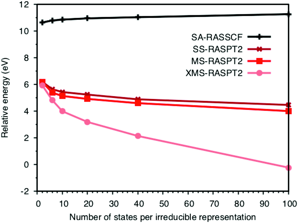 | ||
| Fig. 6 Relative energies of the lowest ungerade LMCT final states of ferrocyanide using different number of states in the SA-RASSCF calculation. The RASPT2 calculations include the same number of states as the corresponding SA-RASSCF calculation. Energies are calculated relative to a single gerade initial state. | ||
As the energies depend on the number of states, simulations must use an equivalent number of initial and final states when comparing with experiment. In ferrocyanide the energy of the first LMCT state is determined from a calculation with one initial state and the six near-degenerate final states of the 8t51ue1g configuration. This translates to the lowest two states in the b1u,2u,3u irreducible representations. The energy of the first LMCT peak is then aligned to this value also in calculations that include the large number of final states required to describe the full spectrum.
Now looking at the RIXS spectra, the number of emission peaks increases when increasing the number of states, see Fig. SI-5 (ESI†). Up to 40 states per irreducible representation are required to get all three peaks. Increasing the number of states further modifies the shape of the final peak but gives no major changes in relative intensities. Further calculations are therefore made using 40 states. The intensities of the SS calculation, which are identical to those from SA-RASSCF, gives an intense middle peak flanked by two peaks of medium intensity, see Fig. 7. Going from SS to MS-RASPT2 calculations redistributes intensity between the low- and mid-energy peaks, with MS getting the right order for the relative intensity of the three peaks. However, as seen in Table 1 above, the intensity of the low-energy peak is now overestimated and the mid-energy peak underestimated. A result between RASSSCF and MS-RASPT2 would give a better agreement with experiment, but there is no theoretical reason to favor SCF over PT2 results, unless the latter had obvious problems with intruder states. XMS could potentially improve the mixing between states, and thus improve the intensity ratios, but going from MS to XMS only has a small effect on the intensities. Instead, the main effect is that the absolute energies are lowered significantly, which gives a poor agreement with experiment. The MS algorithm has therefore been used for the other complexes.
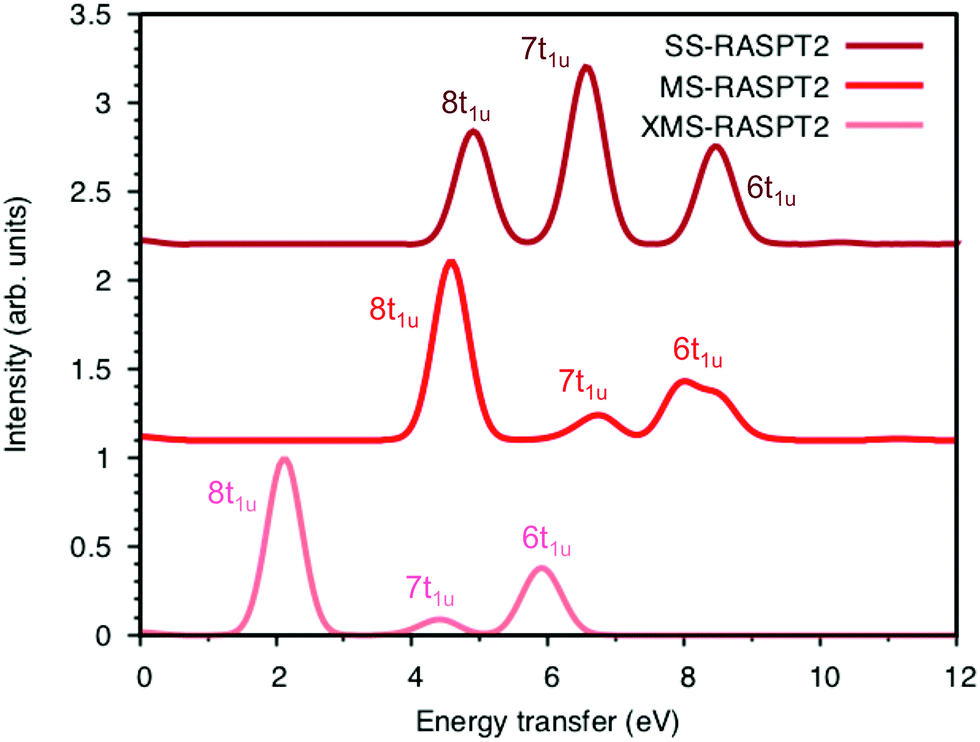 | ||
| Fig. 7 Energy-transfer spectra from the 7113.0 eV pre-edge peak of ferrocyanide using different RASPT2 algorithms. Spectra are calculated with 1 gerade and 40 ungerade valence states without any energy corrections. | ||
To understand the changes in relative intensity, the energy-transfer spectrum was analyzed in more detail. In the dipole approximation, the emission intensity depends on the amount of metal p-character in the orbital from which the electron is removed.78 For valence orbitals, this intensity is dominated by 3p mixing, because of the smaller 4p transition moments. The relative intensity of the state-specific spectrum is reasonably predicted by the amount of 3p character in the SCF orbitals, see Table SI-5 (ESI†). The multi-state spectrum was analyzed through an orbital decomposition analysis, see Fig. 8.40 It shows that even at the highly correlated PT2 level, the peaks are largely associated with individual orbital transitions. The main mixing occurs between states with holes in 8t1u and 7t1u orbitals. This is logical as these orbitals already have mixed 5σ and 1π ligand contributions, see Fig. 4, but even there the weights of the original states are 85% or higher. The limited mixing is also consistent with the relatively small effects on the energies. The spectral changes are thus not due to a complete re-ordering of final states. The large effect of a relatively small mixing comes from the fact that metal-p are minority orbital contributions and can therefore change significantly without any major changes to the states in question. This illustrates the challenges in getting correct intensities and explains the deviations from experiments seen in Table 1.
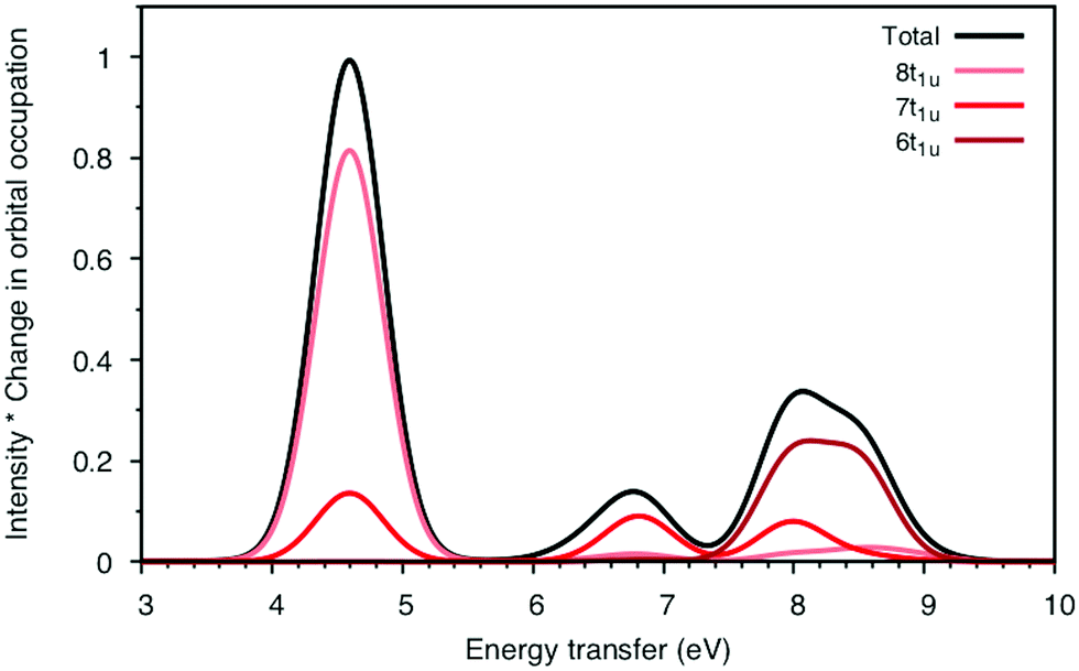 | ||
| Fig. 8 Orbital analysis of the incident energy cut through the 7113.0 eV pre-edge peak of ferrocyanide using MS-RASPT2 and 40 ungerade valence states per irreducible representation. The ratio between total intensity and the orbital values corresponds to the absolute value of the change in orbital occupation number from initial to final states. | ||
To further check the stability of the PT2 treatment, spectra were calculated with different values of both IPEA and imaginary shift, see Fig. SI-6 (ESI†). Increasing the IPEA shift leads to higher energy-transfer values, approx 0.5 eV from 0.25 to 0.5, while also decreasing the split in the high-energy peak. As the energies are underestimated, an increased IPEA shift would lead to better agreement with experiment. The sensitivity to the IPEA shift is due to the initial state being closed shell, while the LMCT states have two open shells. Increasing the imaginary shift leads to similar changes in spectral shape, but has smaller effects on energies.
3.3 Iron(III) and manganese(III) hexacyanide spectra
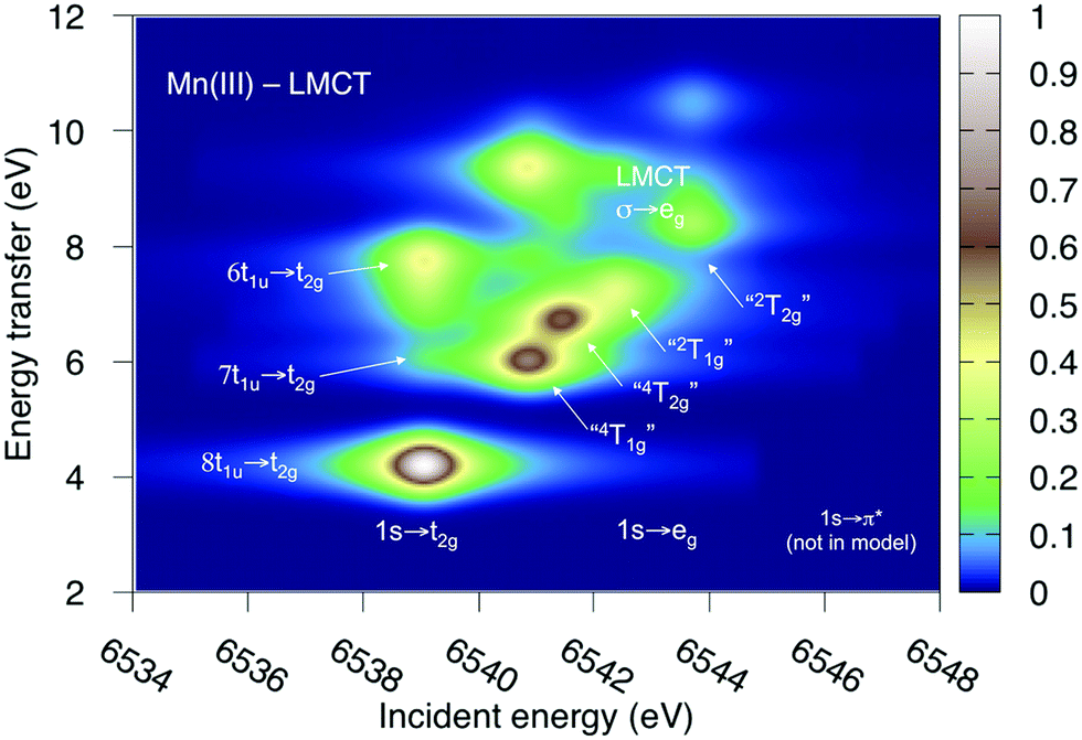
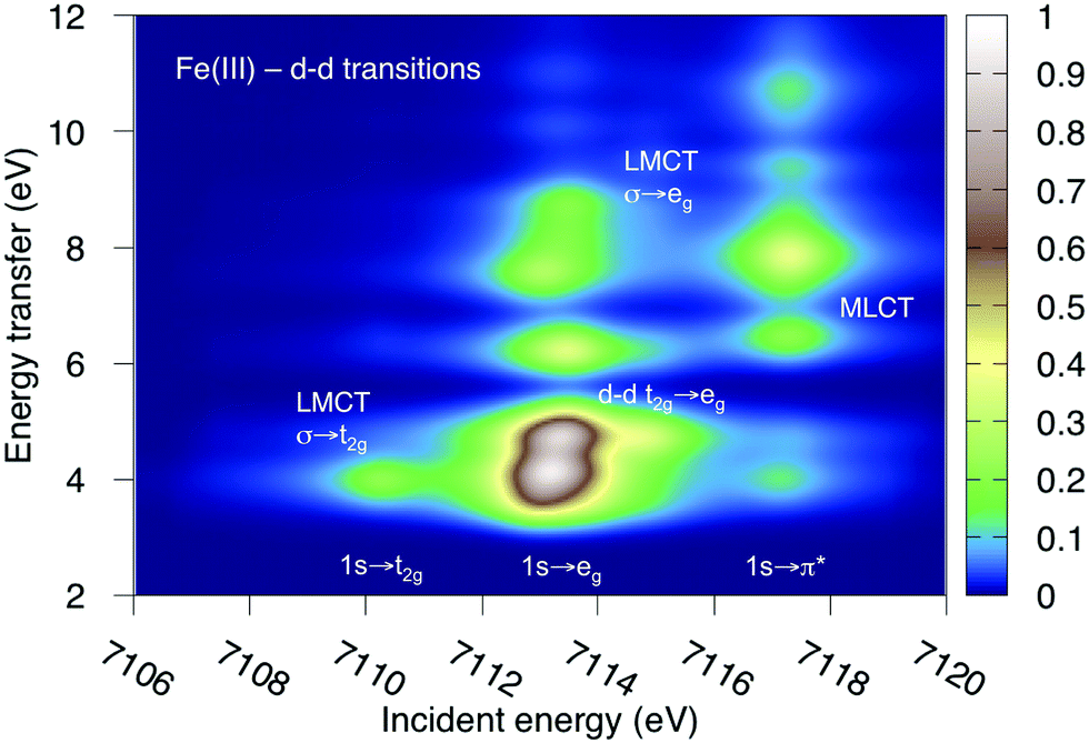
Both ferri- and manganicyanide are open-shell systems, with one and two t2g holes, respectively. The open t2g shell increases the number of pre-edge transitions compared to low-spin iron(II), both through additional orbital excitations and through couplings between open t2g and eg shells.28 The RAS K pre-edge spectrum of manganicyanide is shown in Fig. 9. The corresponding ferricyanide spectrum has been analyzed previously,45 and is shown in Fig. SI-7 (ESI†). Both spectra have low-energy t2g resonances and broader high-energy eg features. In manganicyanide a t2g excitation leaves a single t2g hole, and these states are nearly degenerate. An eg excitation gives two open shells and these states split both due to differences in spin and spatial orientation of the open-shell electrons, see Fig. 9. The combined effects lead to a large number of resonances split over 3 eV. The ferricyanide spectrum is similar in structure, but has a weaker t2g and a narrower eg resonance, see Fig. SI-7 (ESI†).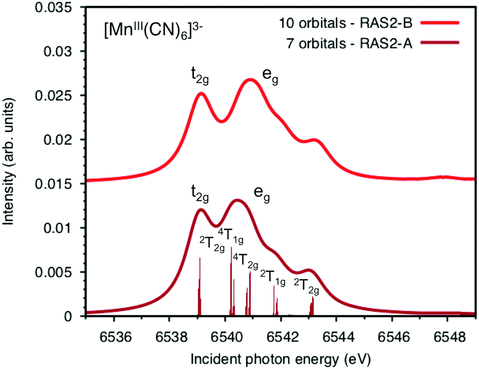 | ||
| Fig. 9 Metal K pre-edge XAS spectra of manganicyanide from MS-RASPT2 calculations using 60 core-excited states and different active spaces. All core-excited states are triplets. The labels for the different transitions correspond to the valence-electron configurations in the d5 Tanabe-Sugano diagram as the exchange interactions with the 1s shell are small. | ||
Compared to experiment, the splitting between t2g and eg resonances is underestimated in both complexes when using the 7-orbital RAS2-A space. This active space allows for correlation between filled and empty orbitals of eg symmetry, but there is no corresponding effect for the t2g shell. Adding three empty t2g-type orbitals, giving the 10-orbital RAS2-B space, leads to a relative stabilization of the t2g resonance by 0.5 eV for both complexes, see Fig. 9 and Fig. SI-7 (ESI†). In both cases, this improves the comparison to experiment, see Table 1. As RIXS spectra have been calculated with the 7-orbital RAS2-A space, a 0.5 eV incident energy correction has been applied to all t2g resonances. Tests with different number of states shows only small effects on the t2g–eg splitting, see Fig. SI-8 (ESI†). Finally, there are no significant differences between spectra calculated with the second-order multipole expansion and the exact semi-classical expression for the wave vector, see Fig. SI-9 (ESI†).
Experimental and simulated RIXS spectra of ferri- and manganicyanide are shown in Fig. 10. As for ferrocyanide, each incident energy resonance has three emission resonances. The experimental spectra show intense low- and high-energy resonances and a weak intermediate resonance. In ferricyanide, the first two energy-transfer resonances in the t2g peak at 3.2 and 4.9 eV, match rather well with UV-Vis resonances at 2.9 and 4.8 eV.27,77 In manganicyanide the first t2g resonance is considerably more intense and the LMCT transitions appear at higher energy transfer values. Here the first LMCT resonance appear at 4.0 eV, again closely matching a UV-Vis resonance (3.9 eV).77
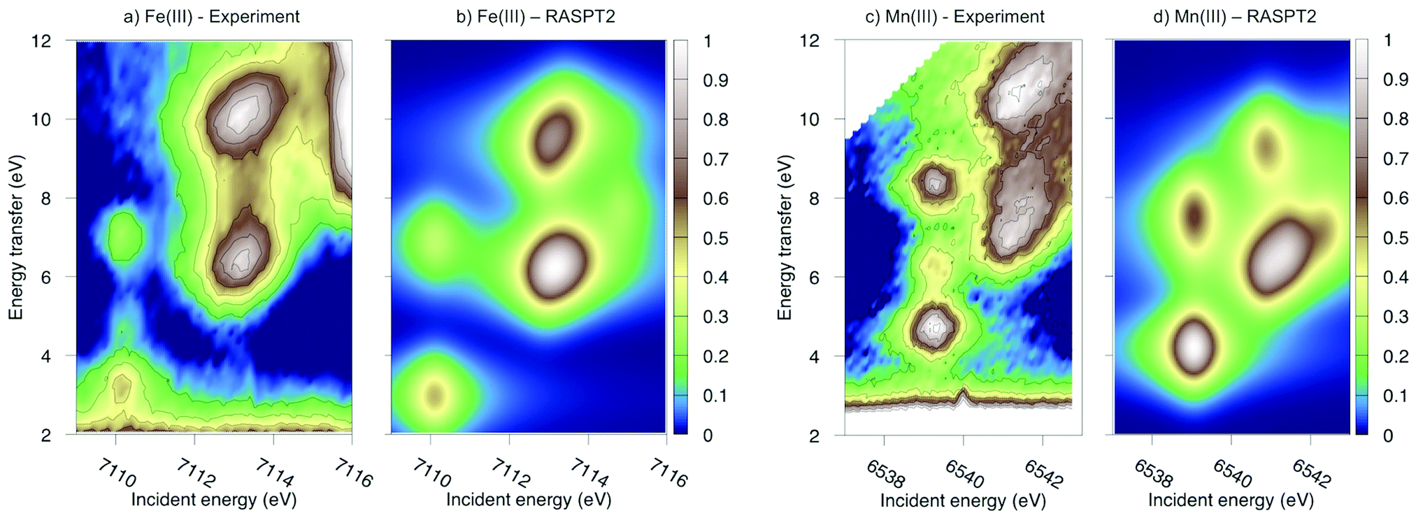 | ||
| Fig. 10 Metal K pre-edge RIXS spectra from experiment and theory. (a) [FeIII(CN)6]3− – Experiment. (b) [FeIII(CN)6]3− – MS-RASPT2. (c) [MnIII(CN)6]3− – Experiment. (d) [MnIII(CN)6]3− – MS-RASPT2. | ||
In the simulated spectra, the intensities closely follow the ferrocyanide results. The SS calculations gives an intense middle peak, which is then reversed in the MS treatment. This gives an intense low-energy, a weak intermediate, and finally a medium-intensity resonance at high energy. Again, the intensity of the low-energy resonance is overestimated and a reduction around 50% would give good results for all complexes, see Table 1. It looks like too much intensity is transferred from the mid-energy resonances because they are so weak that they are not even visible in the simulated spectra plotted with the experimental resolution, and can only be seen in high-resolution spectra, see Fig. 11 for manganicyanide and Fig. SI-10 (ESI†) for ferricyanide. Taking interference into account is not likely to improve these intensity ratios as the effects should be similar for different sets of final LMCT states. When it comes to energies, not only relative but also absolute energies are well described. Almost all peaks show errors of 0.3 eV or less, see Table 1. The main exception is the energy of the highest peak of the eg resonance, which is underestimated by 0.6–0.8 eV in both complexes. The smaller errors in these two systems compared to ferrocyanide is likely due to the fact that both initial and final states are open-shell systems and thus more evenly balanced in the calculations.
 | ||
| Fig. 11 Metal K pre-edge RIXS spectra of manganicyanide from MS-RASPT2 calculations with 0.6 eV experimental broadening in the energy transfer direction. | ||
The consistent treatment of the three complexes shows that simulations can be used to rationalize experimental observations. In the experimental data of the manganese(III) complex, there is clear dispersion in the eg resonance as it extends diagonally in the RIXS plane.23 This is less pronounced in other resonances.27 This dispersion could either be due to a fluorescence signal, or alternatively, several incident energy resonances that are not properly resolved. Simultaneous appearance of resonant and fluorescence signals have been seen in RIXS before,79–81 but not yet in the metal K pre-edge. Therefore, the effect was tentatively explained by a spin splitting of the eg resonance, although a multiplet splitting was also considered.23 The RAS calculations reproduce the prominent dispersion of the manganese(III) eg peak, see Fig. 10b. Analyzing the absorption transitions in Fig. 9, it seems that the 1 eV dispersion comes from the splitting between two valence states, 4T1g and 4t2g, with the same quartet spin coupling but different multiplet couplings, see Fig. 11. The intermediate states with low-spin coupling are both higher in energy and have low transition intensities and do not contribute significantly to the dispersion of the main eg peak.
The experimental manganese(III) spectrum also indicated an MLCT transition at 6545 eV.23 This is not included in the current RIXS simulation as it would require an active space that also contained unfilled ligand orbitals. However, by increasing the number of states in the K pre-edge simulations that uses the larger RAS2-B space, an absorption resonance associated with ligand π* orbitals appear at 6545.6 eV, see Fig. SI-8 (ESI†). The proximity of this peak to the experimental feature tentatively supports the MLCT assignment of this feature.
3.4 RIXS spectra with metal-centered d–d excitations
K-edge RIXS has been successfully used to probe d–d excitations in several systems.21,24,25 The current spectra are dominated by dipole-allowed LMCT transitions and d–d excitations have not been identified. The reason is that for direct RIXS in a centrosymmetric complex, both absorption and emission processes (1s → 3d→ 1s) are electric-dipole forbidden, and the scattering intensity is very low. Looking at Fig. 7, the very weak elastic scattering peak at 0 eV (1s → eg → 1s) has only 2% of the intensity of the most intense LMCT peak. However, for complexes that deviate from centrosymmetry there is significant increase in the cross section due to metal p-mixing into the 3d-type orbitals,28 which applies to both absorption and emission intensities. This could make it possible to study these processes using intense lightsources.To show the potential information in such spectra, the d–d RIXS spectrum of ferri- and manganicyanide, which both have multiple pre-edge resonances, were simulated using the larger RAS2-B 10-orbital valence space. This corresponds to the K pre-edge XAS spectra in Fig. 9 and Fig. SI-7 (ESI†). The ferricyanide spectrum can be directly compared to previous RAS simulations of the Fe L-edge RIXS process.82 It will therefore be discussed in more detail and is shown in Fig. 12, while the manganese(III) spectrum is shown in Fig. SI-11 (ESI†).
 | ||
| Fig. 12 Metal-centered d–d excitations in the K pre-edge RIXS spectra of ferricyanide calculated using MS-RASPT2. | ||
As previously discussed for L-edge RIXS, the scattering process clearly separates different types of excitations along the incident energy axis.2 This means that LMCT and d–d excitations with similar final-state energies can be resolved. First looking at the ferricyanide t2g resonance, there is an energy-transfer feature at 4.0 eV. This emission must come from the occupied σ orbital, leading to a new LMCT (σ → t2g) state. The same transition can be seen in L-edge RIXS. The UV-Vis spectrum also has a resonance in this energy region, but has previously been assigned to a t2u instead of a σ excitation.77 The eg resonance has more energy-loss features, which includes both d–d (t2g → eg) and LMCT excitations. The spectrum is overall very similar to that obtained in L-edge RIXS, although with the strong 2p-3d coupling in the intermediate state replaced with a larger lifetime broadening. As discussed above, for centrosymmetric complexes these excitations would be obscured by the more intense dipole-allowed transitions. For this particular system, the σ → t2g excitation would be hidden by the 8b1u → t2g one. The d–d excitations should appear in a region without dipole-allowed emission, but would be difficult to distinguish from the background noise. At higher incident energies the π* resonance gives rise to several MLCT resonances but these would most likely be hidden under the rising edge.
4 Conclusions
The valence K-edge RIXS spectra of three metal hexacyanide complexes have been modeled using RASPT2. The calculations give a correct description of all LMCT excitations in the spectrum, although the relative intensities and energies are sensitive to the choice of modeling protocol. Inclusion of dynamical correlation is necessary to get reasonable energies of the LMCT final states. In addition, the use of MS-RASPT2 is recommended over SS-RASPT2, despite the increase in computational cost, as it leads to better relative intensities. Hundreds of final states are required to describe emission from all relevant occupied orbitals. As energies depend on the number of states in state-average calculations, the energy scale should be calibrated using equivalent numbers of initial and final states. The need to include all orbitals involved in emission puts severe restrictions on the active space used to describe absorption. This can be corrected for with separate K pre-edge XAS calculations using active spaces designed to better capture correlation with the metal 3d orbitals.The consistent treatment of the three complexes show that the calculations can be used to explain spectral features. The large dispersion in the eg resonance in manganese(III) comes from multiple incident-energy resonances rather than fluorescence. The splittings between these resonances are due to both differences in spin coupling and spatial orientation of holes and electrons, with the largest contributions coming from the latter. The potential for observing d–d excitations is explored, which could be of experimental relevance for non-centrosymmetric systems with intense K pre-edges. These simulations can be useful both when designing and interpreting high-resolution X-ray scattering experiments.
Conflicts of interest
There are no conflicts to declare.Acknowledgements
E. K., M. L., and R. L. acknowledge financial support from the Knut and Alice Wallenberg Foundation (Grant No. KAW-2013.0020). M. D. and M. L. acknowledge support from the Foundation Olle Engkvist Byggmastare. R. L. acknowledge financial support from the Swedish Research Council (VR, grant no. 2016-03398). D. M. and K. G. acknowledge funding from the U.S. Department of Energy, Office of Science, Basic Energy Sciences, Chemical Sciences, Geosciences, and Biosciences Division. Use of the Stanford Synchrotron Radiation Lightsource, SLAC National Accelerator Laboratory, is supported by the U.S. Department of Energy, Office of Science, Office of Basic Energy Sciences under Contract No. DE-AC02-76SF00515. Computations were performed on resources provided by SNIC through the National Supercomputer Centre at Linköping University (Tetralith) under projects snic-2018-3-575 and snic2019-3-586, as well as at Uppsala Multidisciplinary Center for Advanced Computational Science (UPPMAX) under project snic-2019-3-39.References
- L. J. Ament, M. van Veenendaal, T. P. Devereaux, J. P. Hill and J. van den Brink, Rev. Mod. Phys., 2011, 83, 705 CrossRef CAS.
- M. Lundberg and P. Wernet, Light Sources and Free-Electron Lasers: Accelerator Physics, Instrumentation and Science Applications, Springer International Publishing, 2nd edn, 2019, pp. 1–52 Search PubMed.
- C.-C. Kao, W. Caliebe, J. Hastings and J.-M. Gillet, Phys. Rev. B: Condens. Matter Mater. Phys., 1996, 54, 16361 CrossRef CAS PubMed.
- S. Butorin, D. Mancini, J.-H. Guo, N. Wassdahl, J. Nordgren, M. Nakazawa, S. Tanaka, T. Uozumi, A. Kotani, Y. Ma and K. Myano, Phys. Rev. Lett., 1996, 77, 574 CrossRef CAS PubMed.
- S. Butorin, J.-H. Guo, M. Magnuson, P. Kuiper and J. Nordgren, Phys. Rev. B: Condens. Matter Mater. Phys., 1996, 54, 4405 CrossRef CAS PubMed.
- P. Platzman and E. Isaacs, Phys. Rev. B: Condens. Matter Mater. Phys., 1998, 57, 11107 CrossRef CAS.
- A. Kotani and S. Shin, Rev. Mod. Phys., 2001, 73, 203 CrossRef CAS.
- P. Glatzel and U. Bergmann, Coord. Chem. Rev., 2005, 249, 65–95 CrossRef CAS.
- I. Josefsson, K. Kunnus, S. Schreck, A. Föhlisch, F. de Groot, P. Wernet and M. Odelius, J. Phys. Chem. Lett., 2012, 3, 3565–3570 CrossRef CAS PubMed.
- P. Wernet, K. Kunnus, I. Josefsson, I. Rajkovic, W. Quevedo, M. Beye, S. Schreck, S. Gruebel, M. Scholz, D. Nordlund, W. Zhang, R. W. Hartsock, W. F. Schlotter, J. J. Turner, B. Kennedy, F. Hennies, F. M. F. de Groot, K. J. Gaffney, S. Techert, M. Odelius and A. Foehlisch, Nature, 2015, 520, 78–81 CrossRef CAS PubMed.
- A. W. Hahn, B. E. Van Kuiken, V. G. Chilkuri, N. Levin, E. Bill, T. Weyhermüller, A. Nicolaou, J. Miyawaki, Y. Harada and S. DeBeer, Inorg. Chem., 2018, 57, 9515–9530 CrossRef CAS PubMed.
- R. M. Jay, J. Norell, S. Eckert, M. Hantschmann, M. Beye, B. Kennedy, W. Quevedo, W. F. Schlotter, G. L. Dakovski, M. P. Minitti, M. C. Hoffmann, A. Mitra, S. P. Moeller, D. Nordlund, W. Zhang, H. W. Liang, K. Kunnus, K. Kubiček, S. A. Techert, M. Lundberg, P. Wernet, K. Gaffney, M. Odelius and A. Föhlisch, J. Phys. Chem. Lett., 2018, 9, 3538–3543 CrossRef CAS PubMed.
- M. Van Schooneveld and S. DeBeer, J. Electron Spectrosc. Relat. Phenom., 2015, 198, 31–56 CrossRef CAS.
- M. Kubin, J. Kern, M. Guo, E. Källman, R. Mitzner, V. K. Yachandra, M. Lundberg, J. Yano and P. Wernet, Phys. Chem. Chem. Phys., 2018, 20, 16817–16827 RSC.
- J. Hill, C.-C. Kao, W. Caliebe, M. Matsubara, A. Kotani, J. Peng and R. Greene, Phys. Rev. Lett., 1998, 80, 4967 CrossRef CAS.
- S. Galambosi, H. Sutinen, A. Mattila, K. Hämäläinen, R. Sharon, C. Kao and M. Deutsch, Phys. Rev. A: At., Mol., Opt. Phys., 2003, 67, 022510 CrossRef.
- H. Enkisch, C. Sternemann, M. Paulus, M. Volmer and W. Schülke, Phys. Rev. A: At., Mol., Opt. Phys., 2004, 70, 022508 CrossRef.
- Y.-J. Kim, J. Hill, F. Chou, D. Casa, T. Gog and C. Venkataraman, Phys. Rev. B: Condens. Matter Mater. Phys., 2004, 69, 155105 CrossRef.
- D. Qian, Y. Li, M. Hasan, D. Casa, T. Gog, Y.-D. Chuang, K. Tsutsui, T. Tohyama, S. Maekawa and H. Eisaki, et al. , J. Phys. Chem. Solids, 2005, 66, 2212–2215 CrossRef CAS.
- B. C. Larson, W. Ku, J. Z. Tischler, C.-C. Lee, O. Restrepo, A. G. Eguiluz, P. Zschack and K. D. Finkelstein, Phys. Rev. Lett., 2007, 99, 026401 CrossRef CAS PubMed.
- S. Huotari, T. Pylkkaenen, G. Vanko, R. Verbeni, P. Glatzel and G. Monaco, Phys. Rev. B: Condens. Matter Mater. Phys., 2008, 78, 041102 CrossRef.
- F. Vernay, B. Moritz, I. Elfimov, J. Geck, D. Hawthorn, T. Devereaux and G. Sawatzky, Phys. Rev. B: Condens. Matter Mater. Phys., 2008, 77, 104519 CrossRef.
- D. A. Meyer, X. Zhang, U. Bergmann and K. J. Gaffney, J. Chem. Phys., 2010, 132, 134502 CrossRef PubMed.
- J. Kim, Y. Shvyd'ko and S. Ovchinnikov, Phys. Rev. B: Condens. Matter Mater. Phys., 2011, 83, 235109 CrossRef.
- J. Kim, V. V. Struzhkin, S. G. Ovchinnikov, Y. Orlov, Y. Shvyd'ko, M. Upton, D. Casa, A. G. Gavriliuk and S. V. Sinogeikin, EPL, 2014, 108, 37001 CrossRef.
- K. Ishii, M. Kurooka, Y. Shimizu, M. Fujita, K. Yamada and J. Mizuki, J. Phys. Soc. Jpn., 2019, 88, 075001 CrossRef.
- D. A. Meyer, PhD thesis, Stanford University, 2010.
- T. E. Westre, P. Kennepohl, J. G. DeWitt, B. Hedman, K. O. Hodgson and E. I. Solomon, J. Am. Chem. Soc., 1997, 119, 6297–6314 CrossRef CAS.
- P. Glatzel, H. Schroeder, Y. Pushkar, T. Boron III, S. Mukherjee, G. Christou, V. L. Pecoraro, J. Messinger, V. K. Yachandra, U. Bergmann and J. Yano, Inorg. Chem., 2013, 52, 5642–5644 CrossRef CAS PubMed.
- T. Kroll, R. G. Hadt, S. A. Wilson, M. Lundberg, J. J. Yan, T.-C. Weng, D. Sokaras, R. Alonso-Mori, D. Casa, M. H. Upton, B. Hedman, K. O. Hodgson and E. I. Solomon, J. Am. Chem. Soc., 2014, 136, 18087–18099 CrossRef CAS PubMed.
- R. G. Hadt, D. Hayes, C. N. Brodsky, A. M. Ullman, D. M. Casa, M. H. Upton, D. G. Nocera and L. X. Chen, J. Am. Chem. Soc., 2016, 138, 11017–11030 CrossRef CAS PubMed.
- J. J. Yan, T. Kroll, M. L. Baker, S. A. Wilson, R. Decréau, M. Lundberg, D. Sokaras, P. Glatzel, B. Hedman and K. O. Hodgson, et al. , Proc. Natl. Acad. Sci. U. S. A., 2019, 114, 2854–2859 CrossRef PubMed.
- E. Gorelov, A. A. Guda, M. A. Soldatov, S. A. Guda, D. Pashkov, A. Tanaka, S. Lafuerza, C. Lamberti and A. V. Soldatov, Radiat. Phys. Chem., 2018, 108105 CrossRef.
- P. Zimmermann, R. J. Green, M. W. Haverkort and F. M. De Groot, J. Synchrotron Radiat., 2018, 25, 899–905 CrossRef CAS PubMed.
- M. Kang, J. Pelliciari, Y. Krockenberger, J. Li, D. McNally, E. Paris, R. Liang, W. Hardy, D. Bonn and H. Yamamoto, et al. , Phys. Rev. B, 2019, 99, 045105 CrossRef CAS.
- J. Olsen, B. O. Roos, P. Jørgensen and H. J. Å. Jensen, J. Chem. Phys., 1988, 89, 2185–2192 CrossRef CAS.
- P. Å. Malmqvist, A. Rendell and B. O. Roos, J. Phys. Chem., 1990, 94, 5477–5482 CrossRef CAS.
- R. Klooster, R. Broer and M. Filatov, Chem. Phys., 2012, 395, 122–127 CrossRef CAS.
- S. I. Bokarev, M. Dantz, E. Suljoti, O. Kühn and E. F. Aziz, Phys. Rev. Lett., 2013, 111, 083002–083007 CrossRef PubMed.
- R. V. Pinjari, M. G. Delcey, M. Guo, M. Odelius and M. Lundberg, J. Chem. Phys., 2014, 141, 124116 CrossRef PubMed.
- N. Engel, S. I. Bokarev, E. Suljoti, R. Garcia-Diez, K. M. Lange, K. Atak, R. Golnak, A. Kothe, M. Dantz, O. Kühn and E. F. Aziz, J. Phys. Chem. B, 2014, 118, 1555–1563 CrossRef CAS PubMed.
- A. Chantzis, J. K. Kowalska, D. Maganas, S. DeBeer and F. Neese, J. Chem. Theory Comput., 2018, 14, 3686–3702 CrossRef CAS PubMed.
- M. Lundberg and M. Delcey, Transition metals in coordination environments: Computational chemistry and catalysis viewpoints, Springer International Publishing, 2019, vol. 77, pp. 185–217 Search PubMed.
- S. Bernadotte, A. J. Atkins and C. R. Jacob, J. Chem. Phys., 2012, 137, 204106 CrossRef PubMed.
- M. Guo, L. K. Sørensen, M. G. Delcey, R. V. Pinjari and M. Lundberg, Phys. Chem. Chem. Phys., 2016, 18, 3250–3259 RSC.
- M. Guo, E. Källman, L. K. Sørensen, M. G. Delcey, R. V. Pinjari and M. Lundberg, J. Phys. Chem. A, 2016, 120, 5848–5855 CrossRef CAS PubMed.
- L. K. Sørensen, M. Guo, R. Lindh and M. Lundberg, Mol. Phys., 2017, 115, 174–189 CrossRef.
- R. K. Hocking, E. C. Wasinger, F. M. de Groot, K. O. Hodgson, B. Hedman and E. I. Solomon, J. Am. Chem. Soc., 2006, 128, 10442–10451 CrossRef CAS PubMed.
- M. Lundberg, T. Kroll, S. DeBeer George, U. Bergmann, S. A. Wilson, P. Glatzel, D. Nordlund, B. Hedman, K. O. Hodgson and E. I. Solomon, J. Am. Chem. Soc., 2013, 135, 17121–17134 CrossRef CAS PubMed.
- T. Penfold, M. Reinhard, M. Rittmann-Frank, I. Tavernelli, U. Rothlisberger, C. Milne, P. Glatzel and M. Chergui, J. Phys. Chem. A, 2014, 118, 9411–9418 CrossRef CAS PubMed.
- R. V. Pinjari, M. G. Delcey, M. Guo, M. Odelius and M. Lundberg, J. Comput. Chem., 2016, 37, 477–486 CrossRef CAS PubMed.
- S. S. N. Lalithambika, K. Atak, R. Seidel, A. Neubauer, T. Brandenburg, J. Xiao, B. Winter and E. F. Aziz, Sci. Rep., 2017, 7, 1–13 CrossRef PubMed.
- M. Ross, A. Andersen, Z. W. Fox, Y. Zhang, K. Hong, J.-H. Lee, A. Cordones, A. M. March, G. Doumy, S. H. Southworth, M. A. Marcus, R. W. Schoenlein, S. Mukamel, N. Govind and M. Khalil, J. Phys. Chem. B, 2018, 122, 5075–5086 CrossRef CAS PubMed.
- M. Chergui, Coord. Chem. Rev., 2018, 372, 52–65 CrossRef CAS.
- I. Fdez. Galván, M. Vacher, A. Alavi, C. Angeli, F. Aquilante, J. Autschbach, J. J. Bao, S. I. Bokarev, N. A. Bogdanov, R. K. Carlson, L. F. Chibotaru, J. Creutzberg, N. Dattani, M. G. Delcey, S. S. Dong, A. Dreuw, L. Freitag, L. M. Frutos, L. Gagliardi, F. Gendron, A. Giussani, L. González, G. Grell, M. Guo, C. E. Hoyer, M. Johansson, S. Keller, S. Knecht, G. Kovačević, E. Källman, G. Li Manni, M. Lundberg, Y. Ma, S. Mai, J. P. Malhado, P. Å. Malmqvist, P. Marquetand, S. A. Mewes, J. Norell, M. Olivucci, M. Oppel, Q. M. Phung, K. Pierloot, F. Plasser, M. Reiher, A. M. Sand, I. Schapiro, P. Sharma, C. J. Stein, L. K. Sørensen, D. G. Truhlar, M. Ugandi, L. Ungur, A. Valentini, S. Vancoillie, V. Veryazov, O. Weser, T. A. Wesołowski, P.-O. Widmark, S. Wouters, A. Zech, J. P. Zobel and R. Lindh, J. Chem. Theory Comput., 2019, 15, 5925–5964 CrossRef PubMed.
- K. Pierloot, Mol. Phys., 2003, 101, 2083–2094 CrossRef CAS.
- B. O. Roos, R. Lindh, P.-Å. Malmqvist, V. Veryazov and P.-O. Widmark, J. Phys. Chem. A, 2004, 108, 2851–2858 CrossRef CAS.
- B. O. Roos, R. Lindh, P.-Å. Malmqvist, V. Veryazov and P.-O. Widmark, J. Phys. Chem. A, 2005, 109, 6575–6579 CrossRef CAS PubMed.
- F. Aquilante, L. Gagliardi, T. B. Pedersen and R. Lindh, J. Chem. Phys., 2009, 130, 154107 CrossRef PubMed.
- J. Boström, M. G. Delcey, F. Aquilante, L. Serrano-Andrés, T. B. Pedersen and R. Lindh, J. Chem. Theory Comput., 2010, 6, 747–754 CrossRef PubMed.
- P.-Å. Malmqvist, K. Pierloot, A. R. M. Shahi, C. J. Cramer and L. Gagliardi, J. Chem. Phys., 2008, 128, 204109 CrossRef PubMed.
- J. Finley, P.-Å. Malmqvist, B. O. Roos and L. Serrano-Andrés, Chem. Phys. Lett., 1998, 288, 299–306 CrossRef CAS.
- A. A. Granovsky, J. Chem. Phys., 2011, 134, 214113 CrossRef PubMed.
- N. Forsberg and P.-Å. Malmqvist, Chem. Phys. Lett., 1997, 274, 196–204 CrossRef CAS.
- G. Ghigo, B. O. Roos and P.-Å. Malmqvist, Chem. Phys. Lett., 2004, 396, 142–149 CrossRef CAS.
- M. Douglas and N. M. Kroll, Ann. Phys., 1974, 82, 89–155 CAS.
- B. A. Hess, Phys. Rev. A: At., Mol., Opt. Phys., 1986, 33, 3742 CrossRef CAS PubMed.
- P.-Å. Malmqvist and B. O. Roos, Chem. Phys. Lett., 1989, 155, 189–194 CrossRef CAS.
- P.-Å. Malmqvist, B. O. Roos and B. Schimmelpfennig, Chem. Phys. Lett., 2002, 357, 230–240 CrossRef CAS.
- M. G. Delcey, L. K. Sørensen, M. Vacher, R. C. Couto and M. Lundberg, J. Comput. Chem., 2019, 40, 1789–1799 CrossRef CAS PubMed.
- N. H. List, J. Kauczor, T. Saue, H. J. A. Jensen and P. Norman, J. Chem. Phys., 2015, 142, 244111 CrossRef PubMed.
- N. H. List, T. Saue and P. Norman, Mol. Phys., 2017, 115, 63 CrossRef CAS.
- L. K. Sørensen, E. Kieri, S. Srivastav, M. Lundberg and R. Lindh, Phys. Rev. A, 2019, 99, 013419 CrossRef.
- M. Khamesian, I. F. Galván, M. G. Delcey, L. K. Sørensen and R. Lindh, Annual Reports in Computational Chemistry, Elsevier, 2019, vol. 15, pp. 39–76 Search PubMed.
- N. H. List, T. R. L. Melin, M. van Horn and T. Saue, 2020, arXiv preprint, arXiv:2001.10738.
- M. O. Krause and J. Oliver, J. Phys. Chem. Ref. Data, 1979, 8, 329–338 CrossRef CAS.
- J. J. Alexander and H. B. Gray, J. Am. Chem. Soc., 1968, 90, 4260–4271 CrossRef CAS.
- N. Lee, T. Petrenko, U. Bergmann, F. Neese and S. DeBeer, J. Am. Chem. Soc., 2010, 132, 9715–9727 CrossRef CAS PubMed.
- P. Eisenberger, P. Platzman and H. Winick, Phys. Rev. Lett., 1976, 36, 623 CrossRef CAS.
- K. Hamalainen, S. Manninen, P. Suortti, S. Collins, M. Cooper and D. Laundy, J. Phys.: Condens. Matter, 1989, 1, 5955 CrossRef CAS.
- F. Gel'mukhanov and H. Ågren, Phys. Rep., 1999, 312, 87–330 CrossRef.
- K. Kunnus, W. Zhang, M. G. Delcey, R. V. Pinjari, P. S. Miedema, S. Schreck, W. Quevedo, H. Schroeder, A. Föhlisch, K. J. Gaffney, M. Lundberg, M. Odelius and P. Wernet, J. Phys. Chem. B, 2016, 120, 7182–7194 CrossRef CAS PubMed.
Footnote |
| † Electronic supplementary information (ESI) available: Additional figures and tables. See DOI: 10.1039/d0cp01003k |
| This journal is © the Owner Societies 2020 |