DOI:
10.1039/D0SM02130J
(Paper)
Soft Matter, 2021,
17, 3829-3839
Propulsion of an elastic filament in a shear-thinning fluid
Received
1st December 2020
, Accepted 10th February 2021
First published on 12th February 2021
Abstract
Some micro-organisms and artificial micro-swimmers propel at low Reynolds numbers (Re) via the interaction of their flexible appendages with the surrounding fluid. While their locomotion has been extensively studied with a Newtonian fluid assumption, in realistic biological environments these micro-swimmers invariably encounter rheologically complex fluids. In particular, many biological fluids such as blood and different types of mucus have shear-thinning viscosities. The influence of this ubiquitous non-Newtonian rheology on the performance of flexible swimmers remains largely unknown. Here, we present a first study to examine how shear-thinning rheology alters the fluid-structure interaction and hence the propulsion performance of elastic swimmers at low Re. Via a simple elastic swimmer actuated magnetically, we demonstrate that shear-thinning rheology can either enhance or hinder elastohydrodynamic propulsion, depending on the intricate interplay between elastic and viscous forces as well as the magnetic actuation. We also use a reduced-order model to elucidate the mechanisms underlying the enhanced and hindered propulsion observed in different physical regimes. These results and improved understanding could guide the design of flexible micro-swimmers in non-Newtonian fluids.
1 Introduction
Locomotion of micro-swimmers has attracted considerable attention in the past several decades.1–3 These cross-disciplinary efforts have led to not only a better understanding of cell motility in various biological processes4–7 but also design principles that guide the recent development of artificial micro-swimmers.8–12 These artificial micro-swimmers demonstrate vast potential for biomedical applications such as drug delivery and micro-surgery.13–15 A fundamental challenge of swimming at the microscopic scale is the dominance of the viscous force over the inertial force. In this low-Reynolds number regime, the flow exhibits kinematic reversibility, which renders the reciprocal motion (a deformation with time-reversal symmetry) ineffective for self-propulsion as stated by Purcell's scallop theorem.16 For instance, while the periodic opening and closing motion of a scallop's shell or the flapping motion of a rigid body are effective macroscopic propulsion strategies, such a reciprocal motion cannot generate any net translation in a purely viscous fluid at the microscopic scale. To overcome the constraints by the scallop theorem, some microorganisms exploit one or more flexible, slender appendages (called flagella) to produce non-reciprocal deformations along their flagella for self-propulsion.1,4 Inspired by flagellar beating, artificial flexible swimmers consisting of magnetic particles and DNA,17,18 nanowires,19,20 hydrogels,21 and other polymers22,23 have been developed. Propulsion of these flexible structures, also known as elastohydrodynamic propulsion,24–34 emerges as a result of the interplay between hydrodynamic and elastic forces. More recent studies have examined factors such as variable bending stiffness,18,35 intrinsic curvatures,36–38 and magnetic particle geometries39 to enhance elastohydrodynamic propulsion.
While low-Reynolds-number locomotion is relatively well studied with a Newtonian fluid assumption, biological and artificial micro-swimmers invariably encounter complex (non-Newtonian) fluids in their natural habitats and operating environments. These biological fluids often display complex rheological properties such as viscoelasticity and shear-thinning viscosity.40 While locomotion in viscoelastic fluids has been extensively studied,41,42 including the effect of viscoelasticity on flexible swimmers,32,43–47 the effect of shear-thinning rheology has been largely overlooked until more recently. A shear-thinning fluid loses its viscosity with increased shear rates due to changes in the fluid microstructure. Various theoretical and experimental models, including waving sheets,48–50 squirmers,51,52 rotating helices,53,54 and nematodes,55–57 among others,51,58–60 have revealed scenarios where the swimming speed can increase, decrease, or remain unchanged in a shear-thinning fluid relative to that in a Newtonian fluid. Although a wide variety of swimmer models considered in previous studies demonstrate the profound effects of shear-thinning rheology on locomotion, the shape and swimming gaits of these swimmers are prescribed and fixed. How shear-thinning rheology affects the performance of flexible swimmers, whose shapes and gaits are not known a priori but emerge as a result of fluid–structure interactions, remains largely unknown. A list of questions of both fundamental importance and practical significance remain unanswered: how does shear-thinning rheology affect the shape and gait of an elastic swimmer? Do they swim faster or slower in a shear-thinning fluid? What are the mechanisms underlying any enhancement or hindrance of propulsion? How should artificial flexible propellers be designed to maximize their propulsion performance in a shear-thinning fluid? An improved understanding of elastohydrodynamic propulsion in shear-thinning fluids will not only guide the design of this major class of artificial micro-swimmers, but also shed light on how microorganisms may adapt to rheologically complex fluids by better exploiting the fluid–structure interaction for locomotion.
In this work, we present a first study on the effect of shear-thinning rheology on elastohydrodynamic propulsion via a simple yet representative elastic swimmer actuated by an external magnetic field. We note that shear-thinning rheology can induce both local and non-local effects on locomotion.61 The local effect corresponds to the reduction of fluid viscosity due to the increased local shear rates, whereas the non-local effect is concerned with a change in the flow field around the swimmer.50,53,61 As a first step, we focus only on the local effect in this work by adopting a local drag model recently proposed by Riley and Lauga,61 which is effective in capturing the main physical features of swimming in a shear-thinning fluid. The local drag model is based on the Carreau constitutive equation,40 which was shown to describe well the rheological measurements of various biological fluids such as blood,62,63 bile,64 and lung and cervical mucus.49 We will utilize this framework to fill in the gap of missing knowledge on elastohydrodynamic propulsion in a shear-thinning fluid.
The paper is organized as follows. In Section 2 we introduce the model elastic swimmer and formulate the equations governing its elastohydrodynamics in a shear-thinning fluid. In Section 3, we contrast the propulsion performance in a Newtonian fluid (Section 3.1) with that in a shear-thinning fluid (Section 3.2). We also use a reduced-order model in Section 3.3 to further elucidate the essential physics underlying the observed propulsion characteristics in different physical regimes. Finally, we conclude this work with remarks on the limitations and future directions in Section 4.
2 Problem formulation
2.1 Elastic force
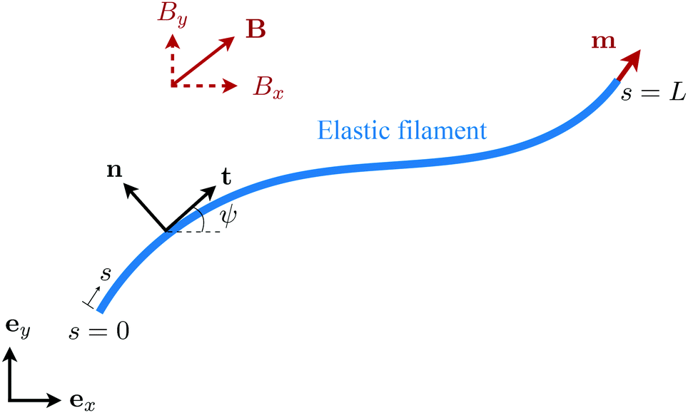
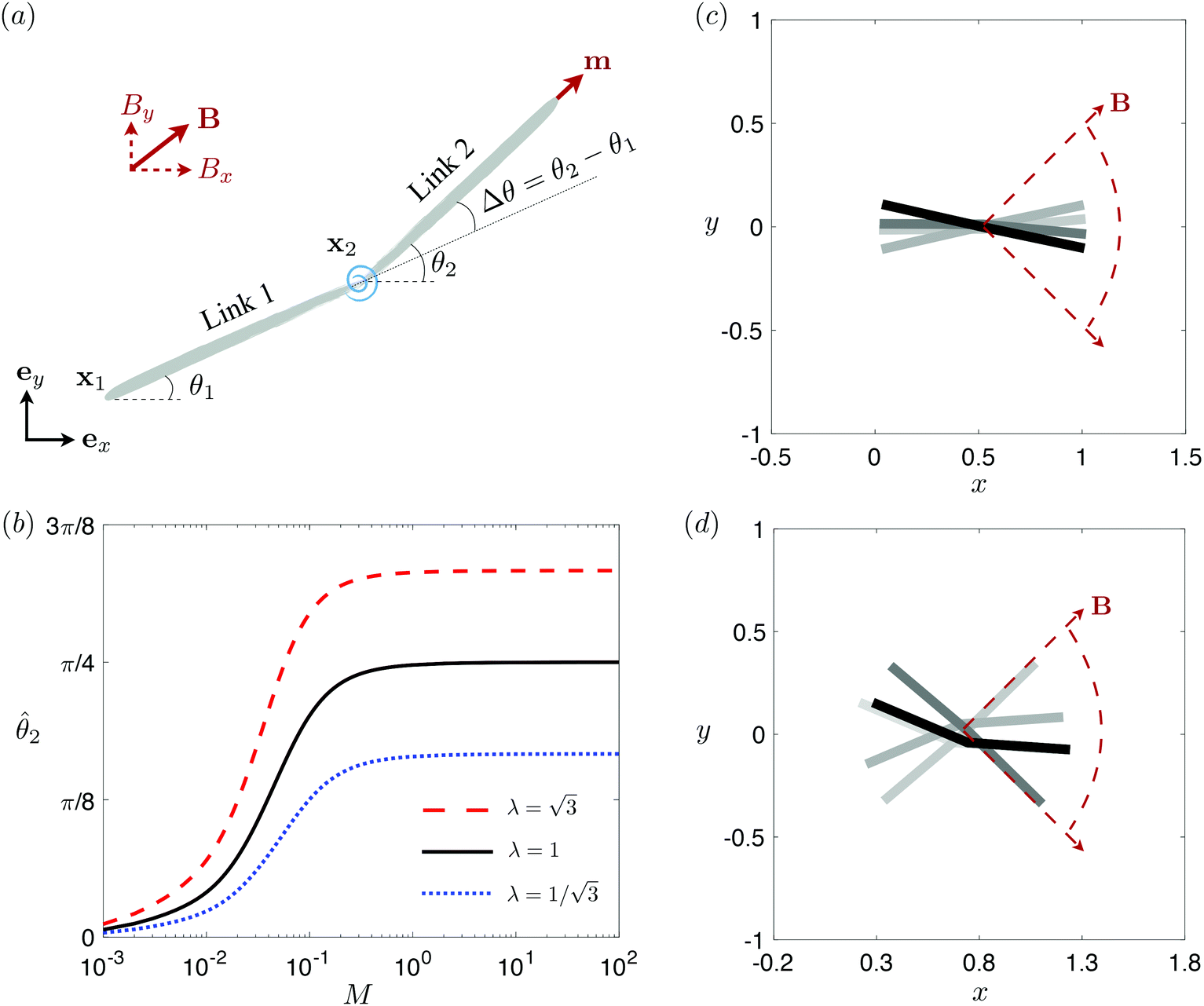
We consider an elastic and inextensible filament of radius a and length L, and assume the filament to be slender, a ≪ L. The position vector of a material point of the filament neutral line in the laboratory frame is denoted as x(s,t), where t represents the time and s ∈ [0,L] is the arclength along the filament. We consider the motion of the filament confined in the x–y plane spanned by the basis vectors ex and ey, with ez = ex × ey. The local unit tangent and normal vectors along the filament are defined as t = xs = cos![[thin space (1/6-em)]](https://www.rsc.org/images/entities/char_2009.gif) ψex + sinψey and n = ez × t, where ψ(s,t) is the angle between the tangent vector t and ex (Fig. 1). The subscript s here denotes differentiation with respect to the arclength.
ψex + sinψey and n = ez × t, where ψ(s,t) is the angle between the tangent vector t and ex (Fig. 1). The subscript s here denotes differentiation with respect to the arclength.
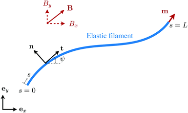 |
| | Fig. 1 Schematic diagram and notation of a model swimmer consisting of an elastic filament with a prescribed magnetic moment m at one of its ends (s = L). Here we examine the effect of shear-thinning rheology on the propulsion of the elastic swimmer under an external magnetic field B. | |
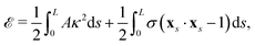
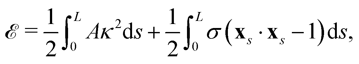
We model the elastic filament as an Euler–Bernoulli beam with an energy functional,65,66
| |  | (1) |
where
A is the bending stiffness,
κ =
xss·
n =
ψs is the local curvature, and
σ(
s,
t) is the Lagrange multiplier enforcing the local inextensibility condition,
xs·
xs = 1. The elastic force density along the filament is obtained by a variational derivative,
| | fe = −δ![[scr E, script letter E]](https://www.rsc.org/images/entities/i_char_e140.gif) /δx = −∂s[Aκsn − τt], /δx = −∂s[Aκsn − τt], | (2) |
where
τ =
σ +
Aκ2 represents the tensile force along the filament. The elastic force density emerging in both normal and tangential directions acts to restore the deformed filament into its undeformed configuration (
i.e., a straight filament). We remark that both bending and inextensibility of the filament contribute to the normal and tensile elastic force.
25,65,66 As a first step, we consider in this work the Euler–Bernoulli beam theory, which does not account for shear and is expected to be less accurate with a large bending displacement. Other geometrically nonlinear rod theories that allow for large displacements (
e.g., Kirchhoff's rod theory) or other modes of deformation (
e.g., Cosserat-type rod theories)
67,68 may be used to extend the present model.
2.2 Fluid force
At low Reynolds number, the hydrodynamic force density along a slender filament fh depends only on the local velocity u in a Newtonian fluid to leading order as described by the local resistive force theory (RFT).69,70 Riley and Lauga61 proposed a modified RFT for locomotion of slender bodies in a shear-thinning fluid as| | | fh = −RC(ξ⊥nn + ξ‖tt)·u, | (3) |
where u = xt, and ξ‖ = 2πη0/[ln(L/a) − 1/2] and ξ⊥ = 4πη0/[ln(L/a) + 1/2] are given by classical RFT results in a Newtonian fluid with dynamic viscosity η0. Here RC is a correction factor accounting for the local shear-thinning effect based on the Carreau constitutive model40,61| | RC = [1 + (λC![[small gamma, Greek, dot above]](https://www.rsc.org/images/entities/i_char_e0a2.gif) avg)2](n−1)/2, avg)2](n−1)/2, | (4) |
where 1/λC represents a critical shear rate beyond which the non-Newtonian behavior becomes significant, n is the shear-thinning index, and the local average shear rate avg is given by| | 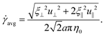 | (5) |
In general, the tangential (u‖ = u·t) and normal (u⊥ = u·n) velocity components and hence the local shear rate vary along a deforming filament. The hydrodynamic force density fh is therefore modified by the spatially and temporally varying correction factor RC. Riley and Lauga61 showed that such modifications cause undulatory swimmers with a prescribed shape to swim slower in a shear-thinning fluid than in a Newtonian fluid. Here we adopt the modified RFT to examine the effect of shear-thinning rheology on the propulsion of a flexible filament, whose shapes are not known a priori but emerge as a result of the interaction between the deforming filament and its surrounding fluid.
2.3 Force balance
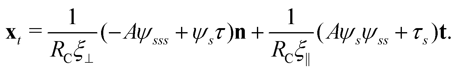
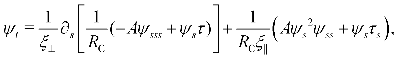
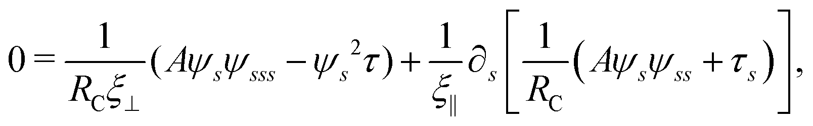
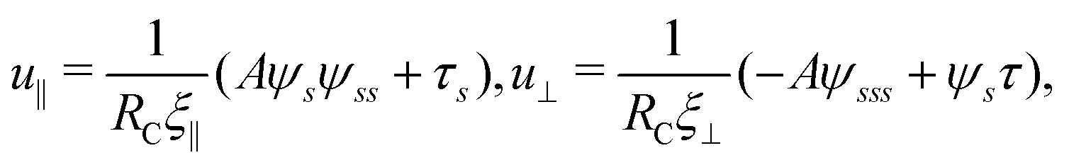
Neglecting the inertia of the filament and its surrounding fluid, there is a local balance between the viscous and elastic forces, fh + fe = 0. The force balance can be inverted as xt = [nn/(RCξ⊥) + tt/(RCξ‖)]·fe, which in terms of the angle formulation is given by| | 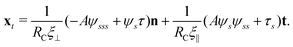 | (6) |
Differentiating eqn (6) with respect to the arc-length s, together with the local inextensibility condition, the normal and tangential components of the resulting equation are, respectively, given by
| |  | (7) |
| |  | (8) |
which can be solved for the tangent angle
ψ(
s,
t) and tensile force
τ(
s,
t). Here the shear-thinning correction factor
RC depends on the local velocity components based on
eqn (4) and (5). Since
u =
xt, the local velocity components can be expressed
viaeqn (6) as
| |  | (9) |
in terms of
RC(
u‖,
u⊥), which depends also on the local velocity components. The correction factor
RC therefore can be determined implicitly as part of the solution to the coupled system of equations above. In the Newtonian limit (
RC = 1) the above coupled nonlinear partial differential equations reduce to the governing equations in the Stokesian limit.
18
2.4 Magnetic actuation
To actuate the swimmer magnetically, we impose a typical external magnetic field B = Bxex + Bysinωtey = bex + bλsinωtey employed in previous studies.17,71–73 The magnetic field consists of a homogeneous static field of strength b in the x-direction and a sinusoidal field of amplitude bλ and frequency ω in the y-direction; here λ = By/Bx compares the magnitude of the sinusoidal field to that of the homogeneous static field. The resulting uniform magnetic field B therefore oscillates around the x-axis. We consider a simple model swimmer consisting of an elastic filament with a magnetic moment m = mt(s = L,t) of strength m prescribed at the right end of the filament in the tangential direction (see Fig. 1 for the setup), where t(s = L,t) = cosψ(s = L,t)ex + sinψ(s = L,t)ey. The uniform external magnetic field thus exerts no net force but a magnetic torque Tm = m × B = Tmez = mb[λcosψ(s = L,t)sinωt − sinψ(s = L,t)]ez at the right end (s = L) of the filament, whose boundary conditions are given by| | | Fext(L,t) = τ(L,t)t − Aψss(L,t)n = 0, | (10) |
| | | Text(L,t) = Aψs(L,t) = Tm. | (11) |
At the other end (s = 0), the filament is free of force and torque:
| | | Fext(0,t) = −τ(0,t)t + Aψss(0,t)n = 0, Text(0,t) = −Aψs(0,t) = 0. | (12) |
2.5 Non-dimensionalization
We non-dimensionalize lengths by L, time by 1/ω, and forces by L2ξ⊥ω. We use the same notations for the corresponding dimensionless variables but with tildes (∼). The governing equations, eqn (7) and (8), in dimensionless forms are given by| |  | (13) |
| |  | (14) |
where| |  | (15) |
Here Sp = L(ξ⊥ω/A)1/4 is the sperm number comparing the magnitude of the viscous to elastic forces, Cu = ωλC is the Carreau number comparing the actuation rate ω with the critical shear rate 1/λC, and γ = ξ⊥/ξ‖ is the drag anisotropy ratio. As a remark, the modified RFT in a shear-thinning fluid is valid for fluids with sufficiently large critical shear rates (1/λC) in order to be consistent with the local nature of the model. We therefore confine our studies only to the dynamics in the low Carreau number regime (Cu ≤ 0.1) in this work. Considering an artificial flexible swimmer with an actuation frequency of O(1 Hz),43 a Cu of 0.1 limits the shear-thinning time scale λC to be O(0.01 s). In practice, we expect Cu to be O(1) or higher, given larger actuation frequency and λC (e.g., λC can range from a tenth of a second to seconds for blood62,63 or larger for other biological fluids49,64). Nevertheless, in the same spirit of other low Cu analyses,49,61,74,75 results in the low Cu regime will reveal the first effects of shear-thinning rheology assuming small departures from the Newtonian limit. The physical insights and qualitative features obtained may be useful in interpreting results at higher Cu as suggested by recent studies.50,52,54
At the actuated end (![[s with combining tilde]](https://www.rsc.org/images/entities/i_char_0073_0303.gif) = 1), the dimensionless boundary conditions for ψ and
= 1), the dimensionless boundary conditions for ψ and ![[small tau, Greek, tilde]](https://www.rsc.org/images/entities/i_char_e0e5.gif) are given by
are given by
| | ψ(1,![[t with combining tilde]](https://www.rsc.org/images/entities/i_char_0074_0303.gif) ) = MSp4[λcosψ(1,)sin − sinψ(1,)], ψ(1,) = 0, (1,) = 0, ) = MSp4[λcosψ(1,)sin − sinψ(1,)], ψ(1,) = 0, (1,) = 0, | (16) |
where
M =
mb/(
L3ξ⊥ω) compares the magnetic to viscous torques. For instance, a typical magnetic torque in previous experiments with magnetic nanowire swimmers
19,20 is given by
mb =
Msam2πLmb, where
Ms = 485 × 10
3 A m
−1 is the spontaneous magnetization of Ni,
am = 100 nm and
Lm = 2 μm are, respectively, the radius and length of the Ni segment, and
b =
O(1 mT) is the magnetic field strength. The characteristic viscous torque acting on the elastic filament is given by
L3ξ⊥ω, where
η0 = 10
−3 Pa s,
a = 50 nm and
L = 4 μm. With an actuation frequency
f of
O(1 Hz)–
O(10 Hz),
M is typically of
O(1) or higher. The value of
M can vary substantially depending on the applied magnetic field strength
b, but a relatively strong magnetic field (
M ≥ 1) is typically applied such that the magnetic segment can follow the magnetic field synchronously [see also
Fig. 3(b) in later discussion].
The dimensionless boundary conditions at the free end ( = 0) are given by
| | | ψ(0,) = 0, ψ(0,) = 0, (0,) = 0. | (17) |
Hereafter we drop the tildes for simplicity and only work with dimensionless variables unless otherwise stated.
We solve the coupled system of nonlinear partial differential equations, eqn (13)–(15), subject to the boundary conditions, eqn (16) and (17) numerically. The numerical simulations are conducted by a finite element method (FEM) based on COMSOL Multiphysics. A backward differentiation formulation is used for time marching the equations. We use 50 to 100 seventh-order Hermite elements to discretize the filament depending on the value of Sp, and a direct solver for solving the linear systems. The computational model is cross-validated against results in the Newtonian limit (Cu = 0) based on a multi-link framework (see Section 3.1 and Appendix for details).
3 Results and discussion
In this section, we will first discuss the propulsion characteristics of the magnetically actuated flexible filament in a Newtonian fluid (Section 3.1). In Section 3.2, we examine how shear-thinning rheology affects the propulsion performance depending on relevant dimensionless groups. Finally, we use a reduced-order model to further elucidate the mechanism underlying the observed propulsion behaviors in Section 3.3.
3.1 Elastohydrodynamic propulsion in a Newtonian fluid
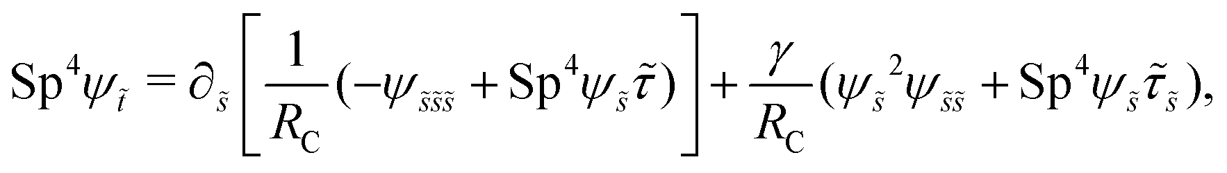
The displacement and shape of the filament  can be obtained from the solution for ψ(s,t) determined in Section 2. We characterize the propulsion performance of the filament by an average swimming speed 〈V〉 = |Δx|/(2π), defined as the magnitude of the filament's mid-point (s = 1/2) displacement Δx = x(1/2,t0 + 2π) − x(1/2,t0) in a period of actuation (2π) divided by the period, where t0 is a sufficiently large time chosen in each simulation such that the displacement per period Δx has approached a steady state. First, we examine the elastohydrodynamic propulsion performance of the filament in a Newtonian fluid (Cu = 0) at different regimes of Sp in Fig. 2. The numerical results based on FEM (black triangles) are compared against the results based on a multi-link model (gray inverted triangles; see Appendix); the results by these two different approaches display excellent agreement.
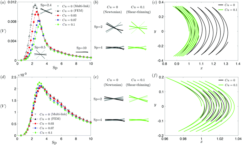 |
| | Fig. 2 Propulsion of a magnetically driven elastic filament in a shear-thinning fluid under a relatively strong [M = 1, panels (a)–(c)] and weak [M = 0.02, panels (d)–(f)] magnetic torques with λ = 1. (a) and (d) Average propulsion speed 〈V〉 of the filament as a function of the sperm number (Sp) for varying Carreau number (Cu). The numerical results based on finite element method (FEM) simulations are compared against the results based on the multi-link model (see Appendix) with 100 links in the Newtonian limit (gray inverted triangles). Insets in (a) display filament deformations over one actuation period T = 2π at equal time intervals (T/4) in the Newtonian limit at various Sp. While the filament generally propels slower in a shear-thinning fluid at most Sp under a strong magnetic torque [M = 1, panel (a)], a small enhancement in the propulsion speed can also occur under a relatively weak magnetic torque [M = 0.02, panel (d)]. (b) and (e) Filament deformations over one actuation period T = 2π at equal time intervals (T/4) in Newtonian and shear-thinning fluids at different Sp; the intensity of color increases as time advances. (c) and (f) The trajectory of the filament's actuated end in Newtonian (solid black, Cu = 0) and shear-thinning (solid green, Cu = 0.1) fluids at Sp = 2 in the first six periods. We set a/L = 1/1000 and a shear-thinning index n = 0.25 in all simulations in this work. | |
The dynamics of a flexible filament in a Newtonian fluid in different regimes of Sp has been characterized in previous studies.17,19,24,29,76 Despite differences in various configurations, the elastohydrodynamic propulsion mechanisms display similar general characteristics as a function of Sp. We illustrate these characteristics with our model swimmer: at low Sp (e.g., Sp = 0.5), the filament is relatively too stiff to undergo significant deformation along the filament; the filament thus behaves largely like a rigid rod performing reciprocal motion [inset, Fig. 2(a)], which leads to ineffective propulsion as constrained by the scallop theorem. As Sp increases, the deformation of the filament enhances its propulsion speed, which reaches a maximum at Sp ≈ 2.4 [see the corresponding filament deformations in Fig. 2(a) inset]. At exceedingly large Sp (e.g., Sp = 10), the filament becomes too soft and hence the deformation is largely localized around the actuated end, as shown in the inset [Fig. 2(a)]; here a large portion of the filament remains horizontal throughout the actuation, which leads to minimal propulsion. A typical swimming trajectory of the filament at Sp = 2 is shown in Fig. 2(c) for the Newtonian case (Cu = 0, black solid line). The filament follows an oscillatory trajectory with net translation in the x-direction.
It is noteworthy that the filament becomes effectively more flexible as Sp increases, which could lead to large deformations that may not be captured quantitatively by the Euler–Bernoulli beam model. Although previous predictions based on the beam model show quantitative agreement with experimental measurements over the experimentally relevant range of Sp,17,19,76 future investigations based on geometrically nonlinear rod theories can be considered to address these limitations.67,68
3.2 Elastohydrodynamic propulsion in a shear-thinning fluid
We next examine how shear-thinning rheology affects the propulsion of the same elastic filament. When the fluid becomes shear-thinning, the local shear-thinning effect can impact the propulsion performance via two different mechanisms. First, given the same shapes and gaits of a swimmer, the local viscosity reduction can still modify the drag and thrust by different amounts, resulting in different propulsion speeds. Such an effect was shown to cause undulatory swimmers with prescribed shapes and gaits to swim slower in a shear-thinning fluid than in a Newtonian fluid.61 The second mechanism, specific to deformable swimmers, is the modification of the shape and gait of the swimmer induced by shear-thinning rheology. Unlike swimmers with prescribed shapes and gaits, the shape and gait of a flexible swimmer are not known a priori but emerge from the interaction between the elastic structure and its surrounding fluid. The shear-thinning viscosity modifies the fluid–structure interaction along the elastic structure (in a non-uniform manner generally) and hence the propulsion performance of the swimmer. In Fig. 2, we depart from the Newtonian limit (Cu = 0) by increasing the value of Cu to probe the effect of shear-thinning rheology on the propulsion speed of the magnetically actuated filament. The propulsion speed as a function of Sp at varying values of Cu is shown in Fig. 2(a) and (d) under, respectively, relatively strong and weak magnetic torques, M.
Under a relatively strong magnetic torque (e.g., M = 1), the propulsion speed generally decreases as the fluid becomes shear-thinning (increasing value of Cu) at most Sp, as shown in Fig. 2(a). This reduction is more substantial at lower Sp (e.g., Sp = 2). Although shear-thinning rheology was shown to reduce the swimming speed for undulatory swimmers of prescribed shapes previously,61 the mechanism underlying the observed reduction here is more complex, because shear-thinning rheology also alters the shape and gait of the swimmer. We visualize the shape of the filament at different time instances in Fig. 2(b), contrasting the deformation in a Newtonian fluid (Cu = 0) with that in a shear-thinning fluid (Cu = 0.1). At Sp = 2, it is apparent that the filament displays less deformation in a shear-thinning fluid than in a Newtonian fluid. In Fig. 2(c), we also compare the swimming trajectories of the filament in a Newtonian (solid black line) and shear-thinning (solid green line) fluids at Sp = 2. While the oscillatory trajectories display similar amplitudes in the y-direction, the net translation in the x-direction is substantially reduced at this Sp.
Although the elastic filament generally propels slower in a shear-thinning fluid under a relatively strong magnetic torque in Fig. 2(a)–(c), we demonstrate in Fig. 2(d)–(f) that shear-thinning rheology can also enhance propulsion under weaker magnetic torques (e.g., M = 0.02). As shown in Fig. 2(d), whether shear-thinning rheology enhances or hinders propulsion also depends on the value of Sp. At lower Sp (e.g., Sp ≲ 3), enhanced propulsion in a shear-thinning fluid is observed, whereas hindered propulsion occurs at higher Sp. Similar to the results in Fig. 2(b), we visualize the shape of the filament at different time instants in a Newtonian and shear-thinning fluids in Fig. 2(e). At Sp = 2, it is apparent that the filament displays a greater range of angular movements in a shear-thinning fluid than in a Newtonian fluid. We also contrast the swimming trajectory at Sp = 2 in a Newtonian fluid (solid black line) with that in a shear-thinning fluid (solid green line) in Fig. 2(f). Unlike the trajectories under a relatively strong magnetic torque shown in in Fig. 2(c), which display similar oscillatory amplitudes, the trajectory of the filament in a shear-thinning fluid has a substantially larger amplitude compared with that in a Newtonian fluid under a relatively weak magnetic torque as shown in in Fig. 2(f).
Taken together, shear-thinning rheology can either increase or decrease the propulsion speed of a flexible swimmer, depending on the specific values of M and Sp. This is unlike the case of undulatory swimmers with prescribed gaits in a shear-thinning fluid,61 where the swimming speeds are systematically lowered. Our observations here thus highlight the effect of gait changes of a flexible swimmer in a shear-thinning fluid (i.e., the second mechanism referred to above) on the propulsion performance. We will further elucidate these results with the use of a reduced-order model in Section 3.3.
3.3 Reduced-order modeling: a two-link model
To better unravel the essential physics underlying elastohydrodynamic propulsion in a shear-thinning fluid, we seek a minimal model reproducing the enhanced and hindered propulsion performance observed in Section 3.2. Specifically, we replace the elastic filament by two rigid links (each of length L/2) connected by a torsional spring with an elastic spring constant k [see Fig. 3(a) for the setup].73,77 We specify the position of the i-th link (i = 1, 2) by the position vector of its left end xi = xiex + yiey and its orientation by the angle θi made between its tangent ti = cosθiex + sinθiey and ex. The position of any point on the i-th link can then be simply given by Xi(s,t) = xi + sti, where s ∈ [0,L/2] is the length along each link. Similar to the original setup (Fig. 1), the same magnetic moment m is prescribed at the right end of link 2 and the left end of link 1 is free of force and torque. Under the same external magnetic field B, we probe the propulsion characteristic of this minimal elastic swimmer in a shear-thinning fluid in this section.
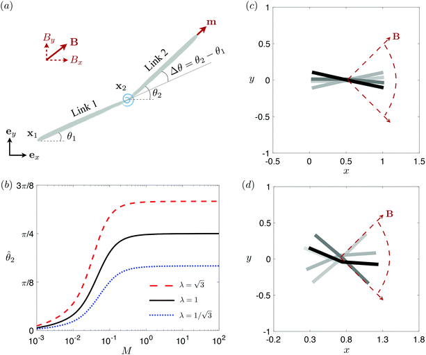 |
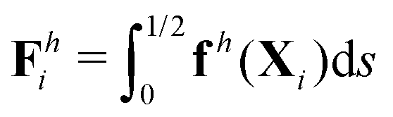
| | Fig. 3 Reduced-order modeling of elastohydrodynamic propulsion. (a) The elastic filament in Fig. 1 is represented by a minimal model consisting of two rigid links connected by a torsional spring. (b) The amplitude of the angle of the actuated link (link 2), ![[small straight theta, Greek, circumflex]](https://www.rsc.org/images/entities/i_char_e12d.gif) 2, as a function of the relative strength of the magnetic torque, M, at different values of λ = By/Bx in a Newtonian fluid with K = 0.1. The amplitude 2 increases with M before leveling off to the maximum value tan−1λ set by the external magnetic field at larger values of M. (c) and (d) The shape of the two-link swimmer over one actuation period T = 2π at equal time intervals (T/4) in a Newtonian fluid; the intensity of color increases as time advances. The dotted lines in (c) and (d) represent the external magnetic field B and the angle spanned by its oscillation for λ = 1. At low M [e.g., M = 0.02 in (c)], the actuated link spans an angle smaller than that spanned by the external magnetic field, 2 < tan−1λ = π/4. At a large M [e.g., M = 1 in (d)], the actuated link follows closely the external magnetic field and attains the same angle spanned by the external magnetic field, 2 < tan−1λ = π/4. 2, as a function of the relative strength of the magnetic torque, M, at different values of λ = By/Bx in a Newtonian fluid with K = 0.1. The amplitude 2 increases with M before leveling off to the maximum value tan−1λ set by the external magnetic field at larger values of M. (c) and (d) The shape of the two-link swimmer over one actuation period T = 2π at equal time intervals (T/4) in a Newtonian fluid; the intensity of color increases as time advances. The dotted lines in (c) and (d) represent the external magnetic field B and the angle spanned by its oscillation for λ = 1. At low M [e.g., M = 0.02 in (c)], the actuated link spans an angle smaller than that spanned by the external magnetic field, 2 < tan−1λ = π/4. At a large M [e.g., M = 1 in (d)], the actuated link follows closely the external magnetic field and attains the same angle spanned by the external magnetic field, 2 < tan−1λ = π/4. | |
We consistently use the same non-dimensionalizations described in Section 2.5 to scale lengths, time, and forces in this reduced-order model. Hereafter we shall work with dimensionless variables only while adopting the same notations for their dimensionless counterparts for convenience. Instead of Sp for a continuous elastic filament, a dimensionless spring constant K = k/(L3ξ⊥ω), which compares the elastic to viscous torques, emerges in this two-link model. Here we note that the dimensionless spring constant K plays a physically similar (but inverse) role to Sp in a continuous filament as shown in Fig. 2. The dynamics of the two-link swimmer is governed by the balance of forces,
and torques (only non-zero in the
z-direction),
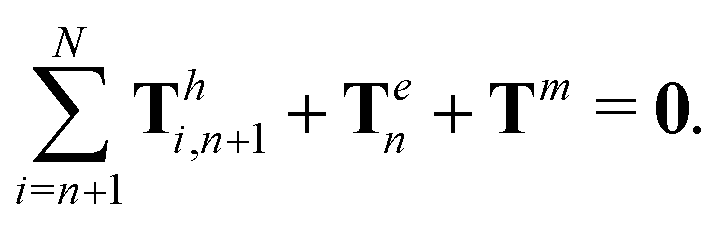
| | | Th1,1 + Th2,1 + Tm = 0, | (19) |
of the overall swimmer, together with the torque balance on the actuated link (link 2),
Here
Tm =
M(
λcos
θ2sin
t − sin
θ2)
ez is the external magnetic torque,

is the hydrodynamic force acting on the
i-th link,
is the hydrodynamic torque generated by the
i-th link about the left end of the
j-th link (
xj), and
Te = −
KΔ
θez is the elastic torque from the torsional spring. With the kinematic constraints
x2 =
x1 + (cos
θ1)/2 and
y2 =
y1 + (sin
θ1)/2, the system of four scalar first-order differential equations [
eqn (18)–(20)] are solved numerically for four unknowns
x1(
t),
y1(
t),
θ1(
t), and
θ2(
t), which completely describe the position and shape of the two-link swimmer with time.
The distinct effects of shear-thinning rheology on the propulsion performance under strong and weak magnetic torques revealed in Fig. 2 can be better understood by examining the response of the two-link swimmer to the magnetic actuation. In this two-link model [Fig. 3(a)], the actuation comes from link 2 attempting to follow the external magnetic field (characterized by the angle θ2), whereas link 1 responds elastically to the actuation via the torsional spring (characterized by the relative angle Δθ = θ2 − θ1). The propulsion behavior of the two-link swimmer can be described in terms of the amplitude of the angles 2 = max(θ2) and  . Therefore, understanding the effect of shear-thinning rheology on elastohydrodynamic propulsion can be reduced to elucidating how 2 and
  are modified in a shear-thinning fluid in various scenarios.
The maximum angle 2 spanned by the actuated link (link 2) under the oscillating magnetic field largely depends on the relative strength of the magnetic torque, M. We first examine this dependence in a Newtonian fluid in Fig. 3(b). At low M, the amplitude 2 increases with M before leveling off to the maximum angle (tan−1λ) set by the external magnetic field (λ = By/Bx) at large M ≥ 1. For instance, Fig. 3(c) displays the time evolution of a two-link swimmer under a weak magnetic torque (M = 0.02 and λ = 1), where the actuated link spans an angle much smaller than tan−1λ = π/4; essentially, the magnetic torque is relatively too weak to actuate the link fast enough to follow closely the oscillatory magnetic field. On the other hand, when the magnetic torque is relatively strong (e.g., M ≥ 1), the actuated link follows the magnetic field almost synchronously, spanning the maximum angle 2 ≈ tan−1λ = π/4 as shown in Fig. 3(d); in this synchronous regime, a further increase in the strength of the magnetic torque M has little effect on the dynamics of the actuated link and hence that of the swimmer. The difference in the dynamics of the actuated link under relatively weak and strong magnetic torques is crucial in understanding the hindered and enhanced propulsion observed in a shear-thinning fluid. We next discuss how shear-thinning rheology modifies the propulsion of the two-link swimmer under relatively weak and strong magnetic torques in terms of 2 and  and compare the results with that for a continuous filament in Fig. 2.
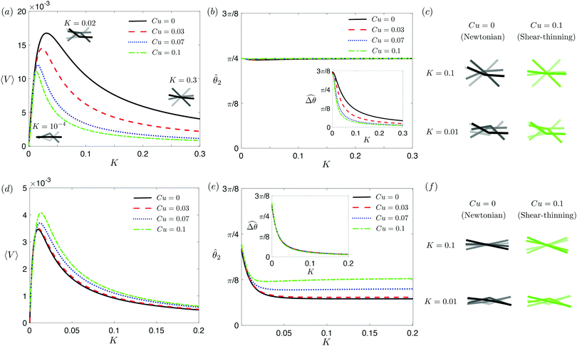
3.3.1 Propulsion at large M.
Under a relatively strong magnetic torque (e.g., M = 1), shear-thinning rheology generally reduces the propulsion speed of the two-link swimmer at most K as shown in Fig. 4(a), similar to the results for a continuous filament in Fig. 2(a). First, we examine how shear-thinning rheology alters the gaits (characterized by 2 and  ) and hence the propulsion speed of a two-link swimmer. At large M, due to the dominance of the magnetic actuation on the dynamics of the actuated link, reduced viscous torques in a shear-thinning fluid has little influence on the actuation angle 2 [Fig. 4(b)]. The actuated link spans approximately the same maximum angle 2 = tan−1λ = π/4 dictated by the external magnetic field (λ = By/Bx = 1) at different values of Cu. Modifications on the swimming gait in this large-M regime therefore stem only from changes in the relative angle
  in a shear-thinning fluid [inset, Fig. 4(b)]. As Cu increases, the shear-thinning viscosity reduces the viscous torque; a smaller elastic torque is thus required to balance the viscous torque, leading to a reduced amplitude of the relative angle
  . The effect is analogous to a further increase in the spring constant K. The two-link swimmer hence behaves increasingly more like a rigid rod in a shear-thinning fluid as Cu increases [Fig. 4(c), K = 0.1], which acts to hinder propulsion. The same mechanism contributes to the decrease in propulsion speed for a continuous filament at high M [Fig. 2(a)], where shear-thinning rheology reduces the deformation along the filament owing to the reduced viscous forces [see Fig. 2(a) and (b)]. As a remark, even without any shape changes, an undulatory swimmer with the same gaits can swim slower in a shear-thinning fluid, because thrust is reduced to a larger extent than drag for undulatory swimmers.61 This latter effect combines with the effect due to gait changes to significantly reduce the propulsion performance at larger values of K in Fig. 4(a) [or smaller values of Sp in Fig. 2(a)]. On the other hand, at smaller values of K (e.g., K = 0.01), propulsion is relatively ineffective in the Newtonian limit due to the dominance of the viscous effect over the elastic effect on the dynamics of link 1. In this regime, the reduction in the viscous effect caused by shear-thinning rheology indeed allows more effective swimming gaits to emerge (the effect is analogous to an increased K). The two mechanisms, which act in tandem to hinder propulsion at large K, now counter-act and lead to less significant changes in the overall propulsion performance in the small K (or large Sp) regime.
 |
| | Fig. 4 Propulsion of a magnetically-driven two-link swimmer in a shear-thinning fluid under relatively strong [M = 1, panels (a)–(c)] and weak [M = 0.02, panels (d)–(f)] magnetic torques with λ = 1. (a) and (d) Average propulsion speed 〈V〉 of the swimmer as a function of the dimensionless spring constant (K) for varying Carreau number (Cu). Insets in (a) display the shape of the swimmer over one actuation period T = 2π at equal time intervals (T/4) in the Newtonian limit at various K. We note that K of a two-link swimmer plays a physically similar (but inverse) role to Sp of a continuous filament as shown in Fig. 2. Similar to the results for a continuous filament, while the two-link swimmer generally propels slower in a shear-thinning fluid under a relatively strong magnetic torque [M = 1, panel (a)], enhanced propulsion can also occur under a relatively weak magnetic torque [M = 0.02, panel (d)]. (b) and (e) The amplitude of the actuated link's angle (2) and that of the relative angle ( insets) as a function of K at varying Cu. (c) and (f) The shape of the swimmer over one actuation period T = 2π at equal time intervals (T/4) in Newtonian and shear-thinning fluids at different K; the intensity of the color increases as time advances. insets) as a function of K at varying Cu. (c) and (f) The shape of the swimmer over one actuation period T = 2π at equal time intervals (T/4) in Newtonian and shear-thinning fluids at different K; the intensity of the color increases as time advances. | |
3.3.2 Propulsion at small M.
The propulsion performance of the two-link swimmer is modified by shear-thinning rheology in a qualitatively different manner at small M [Fig. 4(d)], where enhanced propulsion can occur. We attribute the difference to the distinct ways shear-thinning rheology alters the swimming gaits at small and large M [compare Fig. 4(b) and (e)]. While 2 at large M always attains the maximum angle tan−1λ = π/4 allowed by the external magnetic field, the actuated link spans angles that are considerably smaller (2 ≪ π/4) under a relatively weak magnetic torque (e.g., M = 0.02). The viscous effect dominates the dynamics of the actuated link in this regime and limits the amplitude of its angular movements, 2. When the fluid becomes shear-thinning, the reduced viscous effect on the actuated link allows the link to span larger angles 2 as Cu increases [Fig. 4(e)]. We argue that this increased angle of actuation [apparent in the visualizations shown in Fig. 4(f) at K = 0.1], induced by shear-thinning rheology at small M, is responsible for the enhanced propulsion observed in Fig. 4(d). A similar effect is at play for a continuous filament actuated with a small M [Fig. 2(e), Sp = 2], where the filament's actuated (right) end displays an increased amplitude and hence the propulsion speed in a shear-thinning fluid [Fig. 2(d)]. It is noteworthy that the increase in the actuation amplitude becomes less significant at lower values of K (or higher Sp); in this regime, the other shear-thinning effect unrelated to gait changes but a greater reduction in thrust than drag for undulatory swimmers,61 which acts to hinder propulsion, may become more important. A reduction in the propulsion speed is apparent for a continuous filament at high Sp as shown in Fig. 2(d).
We summarize the essential physical pictures at large (Section 3.3.1) and small (Section 3.3.2) M as follows. Via the two-link model, we reduce the description of a flexible swimmer into two portions: the portion responsible for actuation (link 2) and the portion responsible for the elastic response (link 1). Under a relatively small magnetic torque (M ≪ 1), the amplitude of actuation is suppressed by excessively large viscous effects on the actuated portion. Here shear-thinning rheology enables a larger amplitude of actuation (2) by reducing the viscous effect, which leads to enhanced propulsion in this regime. In contrast, under a relatively strong magnetic torque (M ≥ 1), the actuated portion already maximizes the amplitude of actuation allowed by the magnetic field; shear-thinning rheology hence alters the swimming gait only via changes in the relative angle  . Shear-thinning rheology generally reduces
  because a smaller elastic torque is required to balance the reduced viscous torque in a shear-thinning fluid. At higher values of K, a reduced
  makes the two-link swimmer behave more like a rigid rod with hindered propulsion performance. On the other hand, at smaller values of K, a reduced
  could act to enhance propulsion by allowing the two-link swimmer to deviate from relatively ineffective gaits in a Newtonian fluid in this regime. Overall, while these gait changes induced by shear-thinning rheology affect propulsion, we also note that, even without inducing any gait changes, shear-thinning rheology can also hinder the propulsion of undulatory swimmers by reducing the thrust more than drag.61 This later effect can act in tandem or counter-act with the effect due to gait changes to enhance or hinder propulsion by varying extents in different physical regimes. Taken together, the physical picture presented here captures qualitatively the behaviors observed for a continuous filament.
4 Concluding remarks
Unlike previous studies on locomotion in shear-thinning fluids with prescribed swimming gaits, here the shapes of an elastic swimmer are not known a priori but emerge due to the interplay of the deforming body and its surrounding fluid. In this work, we present a first study to elucidate how shear-thinning rheology affects elastohydrodynamic propulsion at low Reynolds numbers. Via a simple model consisting of an elastic filament actuated by an external magnetic field, we demonstrated that such an elastohydrodynamic swimmer can propel either faster or slower in a shear-thinning fluid than in a Newtonian fluid in different physical regimes characterized by M and Sp. To complement the results for a continuous filament, we also used a two-link model to reproduce and interpret the observed hindered (enhanced) propulsion under relatively strong (weak) magnetic torques. Our results also show that when a relatively strong magnetic torque is used in practice, the optimal Sp maximizing the propulsion performance increased with Cu. These findings call for future experimental investigations of magnetic flexible propellers in shear-thinning fluids. In addition, future works incorporating various motor coordination schemes78,79 into the current elastohydrodynamic framework may also shed light on cell motility in biological fluids displaying shear-thinning viscosity.
We discussed several limitations in this work, which provide directions for subsequent studies. First, as a first step we considered a local drag model here and therefore only accounted for the local shear-thinning effect. This also confines the validity of our results to the small Carreau number regime to be consistent with the local nature of the model.61 The change in the flow field due to non-local shear-thinning effects and non-local hydrodynamic interactions remains to be investigated. Second, for simplicity we prescribed a magnetic moment at one of the filament's end as a minimal model of a magnetic swimmer in this work. We have therefore ignored the hydrodynamic effect of the magnetic head geometry, which is another design parameter for optimizing the propulsion performance of magnetic swimmers.39 Finally, we note that magnetic actuation is considered here for its common use as an actuation mechanism for artificial micro-swimmers.80,81 The same framework can be employed to consider other types of boundary or distributed actuation mechanisms that are more relevant to biological swimmers.25,82–84 We believe that the essential physical pictures discussed in this work could still be generally useful in interpreting the effect of shear-thinning rheology in other swimmer configurations.
Conflicts of interest
There are no conflicts to declare.
Appendix: multi-link model
In this appendix, we consider a framework based on a multi-link discretization85–87 of an elastic filament. We use the results from this multi-link model to cross-validate the numerical solutions obtained by the FEM described in Section 2.5 in the Newtonian limit [gray inverted triangles in Fig. 2(a) and (d)]. The multi-link model may also be considered as a logical extension of the two-link model considered in Section 3.3. In this multi-link model, an elastic filament of length L is discretized by a chain of N rigid links of equal length ![[small script l]](https://www.rsc.org/images/entities/char_e146.gif) = L/N (Fig. 5). These links are serially connected together by N − 1 torsional springs with the same spring constant k. Similar to the two-link model in Section 3.3, the position of the i-th link (i = 1,2,…,N) is specified by the position vector of its left end xi = xiex + yiey, and its orientation is specified by the angle θi made between its unit tangent ti = cosθiex + sinθiey and ex. The position vector along the i-th link is therefore given by Xi = xi + sti, where the archlength s ∈ [0,]. Similar to the continuous case, the unit normal is given by ni = ez × ti. The discretization follows kinematic constraints given by xi+1 = xi + [cosθi,sinθi] between successive links. The description of hydrodynamic force on the i-th link follows the same form in the two-link swimmer as
= L/N (Fig. 5). These links are serially connected together by N − 1 torsional springs with the same spring constant k. Similar to the two-link model in Section 3.3, the position of the i-th link (i = 1,2,…,N) is specified by the position vector of its left end xi = xiex + yiey, and its orientation is specified by the angle θi made between its unit tangent ti = cosθiex + sinθiey and ex. The position vector along the i-th link is therefore given by Xi = xi + sti, where the archlength s ∈ [0,]. Similar to the continuous case, the unit normal is given by ni = ez × ti. The discretization follows kinematic constraints given by xi+1 = xi + [cosθi,sinθi] between successive links. The description of hydrodynamic force on the i-th link follows the same form in the two-link swimmer as| | 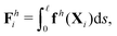 | (21) |
where fh is the hydrodynamic force density given by the resistive force theory [eqn (3)]. Similarly, the hydrodynamic torque on the i-th link about xj follows the same form in the two-link swimmer as| |  | (22) |
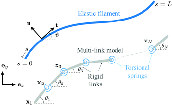 |
| | Fig. 5 Schematic diagram illustrating a multi-link discretization of an elastic filament and notations. | |
The dynamics of the multi-link model is governed by the overall balance of force
| |  | (23) |
and torque
| |  | (24) |
of the
N-link assembly, as well as the torque balances on the assembly minus the
n-th link (
n = 1,…,
N− 1)
| |  | (25) |
Here the elastic torque by the torsional spring
Ten = −
k(
θn+1 −
θn)
ez and the magnetic torque
Tm =
mb[
λcos
θNsin
ωt − sin
θN]
ez act on the right end of the
N-link. These force and torque balances together with the kinematic constraints between successive links form a system of first-order ordinary differential equations that can be solved numerically to determine the unknowns,
xi and
θi. The spring constant in the multi-link model
k =
A/(
L/
N) can be adjusted to represent an elastic filament with bending stiffness
A.
86,87 For a sufficiently large number of links [
e.g.,
N = 100 in
Fig. 2(a) and (d)], results from the
N-link model display excellent agreement with results from FEM simulations. As a remark, the multi-link model may also be relevant to modeling the dynamics of a single polymer/DNA when intrachain hydrodynamic interactions are weak.
88–90
Acknowledgements
O. S. P. acknowledges support from the National Science Foundation (Grant Numbers 1931292 and 1830958). L. Z. acknowledges the start-up grant (R-265-000-696-133) from the National University of Singapore. Computational resources from the WAVE computing facility (enabled by the Wiegand Foundation) at Santa Clara University and the National Supercomputing Centre, Singapore are also gratefully acknowledged.
References
- E. Lauga and T. R. Powers, Rep. Prog. Phys., 2009, 72, 096601 CrossRef.
- M. Sitti, Nature, 2009, 458, 1121–1122 CrossRef CAS PubMed.
- J. Elgeti, R. G. Winkler and G. Gompper, Rep. Prog. Phys., 2015, 78, 056601 CrossRef CAS PubMed.
- L. J. Fauci and R. Dillon, Annu. Rev. Fluid Mech., 2006, 38, 371–394 CrossRef.
- E. Gaffney, H. Gadêlha, D. Smith, J. Blake and J. Kirkman-Brown, Annu. Rev. Fluid Mech., 2011, 43, 501–528 CrossRef.
- J. M. Yeomans, D. O. Pushkin and H. Shum, Eur. Phys. J.: Spec. Top., 2014, 223, 1771–1785 Search PubMed.
- H. Gadêlha, P. Hernández-Herrera, F. Montoya, A. Darszon and G. Corkidi, Sci. Adv., 2020, 6, eaba5168 CrossRef PubMed.
- J. J. Abbott, K. E. Peyer, M. C. Lagomarsino, L. Zhang, L. Dong, I. K. Kaliakatsos and B. J. Nelson, Int. J. Robot. Res., 2009, 28, 1434–1447 CrossRef.
- S. J. Ebbens and J. R. Howse, Soft Matter, 2010, 6, 726–738 RSC.
- S. Sengupta, M. E. Ibele and A. Sen, Angew. Chem., Int. Ed., 2012, 51, 8434–8445 CrossRef CAS PubMed.
- J. L. Moran and J. D. Posner, Annu. Rev. Fluid Mech., 2017, 49, 511–540 CrossRef.
- C. Hu, S. Pané and B. J. Nelson, Annu. Rev. Control Robot. Auton. Syst., 2018, 1, 53–75 CrossRef.
- B. J. Nelson, I. K. Kaliakatsos and J. J. Abbott, Annu. Rev. Biomed. Eng., 2010, 12, 55–85 CrossRef CAS PubMed.
- J. Wang and W. Gao, ACS Nano, 2012, 6, 5745–5751 CrossRef CAS PubMed.
- M. Medina-Sánchez and O. G. Schmidt, Nature, 2017, 545, 406–408 CrossRef PubMed.
- E. M. Purcell, Am. J. Phys., 1977, 45, 3–11 CrossRef.
- R. Dreyfus, J. Baudry, M. L. Roper, M. Fermigier, H. A. Stone and J. Bibette, Nature, 2005, 437, 862–865 CrossRef CAS PubMed.
- A. M. Maier, C. Weig, P. Oswald, E. Frey, P. Fischer and T. Liedl, Nano Lett., 2016, 16, 906–910 CrossRef CAS PubMed.
- O. S. Pak, W. Gao, J. Wang and E. Lauga, Soft Matter, 2011, 7, 8169–8181 RSC.
- W. Gao, D. Kagan, O. S. Pak, C. Clawson, S. Campuzano, E. Chuluun-Erdene, E. Shipton, E. E. Fullerton, L. Zhang, E. Lauga and J. Wang, Small, 2012, 8, 460–467 CrossRef CAS PubMed.
- H.-W. Huang, F. E. Uslu, P. Katsamba, E. Lauga, M. S. Sakar and B. J. Nelson, Sci. Adv., 2019, 5, eaau1532 CrossRef PubMed.
- B. J. Williams, S. V. Anand, J. Rajagopalan and M. T. A. Saif, Nat. Commun., 2014, 5, 3081 CrossRef PubMed.
- I. S. M. Khalil, A. F. Tabak, Y. Hamed, M. E. Mitwally, M. Tawakol, A. Klingner and M. Sitti, Adv. Sci., 2018, 5, 1700461 CrossRef PubMed.
- C. H. Wiggins and R. E. Goldstein, Phys. Rev. Lett., 1998, 80, 3879–3882 CrossRef CAS.
- S. Camalet and F. Jülicher, New J. Phys., 2000, 2, 24 CrossRef.
- C. P. Lowe, Phil. Trans. R. Soc. B, 2003, 358, 1543–1550 CrossRef.
- M. Manghi, X. Schlagberger and R. R. Netz, Phys. Rev. Lett., 2006, 96, 068101 CrossRef PubMed.
- E. Gauger and H. Stark, Phys. Rev. E, 2006, 74, 021907 CrossRef PubMed.
- E. Lauga, Phys. Rev. E, 2007, 75, 041916 CrossRef PubMed.
- N. Coq, O. du Roure, J. Marthelot, D. Bartolo and M. Fermigier, Phys. Fluids, 2008, 20, 051703 CrossRef.
- E. E. Keaveny and M. R. Maxey, J. Fluid Mech., 2008, 598, 293–319 CrossRef.
- H. C. Fu, C. W. Wolgemuth and T. R. Powers, Phys. Rev. E, 2008, 78, 041913 CrossRef PubMed.
- B. Qian, T. R. Powers and K. S. Breuer, Phys. Rev. Lett., 2008, 100, 078101 CrossRef PubMed.
- Y. Mirzae, B. Y. Rubinstein, K. I. Morozov and A. M. Leshansky, Front. Robot. AI, 2020, 7, 152 Search PubMed.
- Z. Peng, G. J. Elfring and O. S. Pak, Soft Matter, 2017, 13, 2339–2347 RSC.
- Z. Liu, F. Qin, L. Zhu, R. Yang and X. Luo, Phys. Fluids, 2020, 32, 041902 CrossRef CAS.
- S. Mohanty, Q. Jin, G. P. Furtado, A. Ghosh, G. Pahapale, I. S. M. Khalil, D. H. Gracias and S. Misra, Adv. Intell. Syst., 2020, 2, 2000064 CrossRef.
- Z. Liu, F. Qin and L. Zhu, Phys. Rev. Fluids, 2020, 5, 124101 CrossRef.
- H. Gadêlha, Regul. Chaot. Dyn., 2013, 18, 75–84 CrossRef.
-
R. B. Bird, R. C. Armstrong and O. Hassager, Dynamics of polymeric liquids. Fluid mechanics, John Wiley and Sons Inc., New York, vol. 1, 1987 Search PubMed.
-
J. Sznitman and P. E. Arratia, Complex Fluids in Biological Systems, Springer, New York, 2015, pp. 245–281 Search PubMed.
-
G. J. Elfring and E. Lauga, Complex Fluids in Biological Systems, Springer, New York, 2015, pp. 283–317 Search PubMed.
- J. Espinosa-Garcia, E. Lauga and R. Zenit, Phys. Fluids, 2013, 25, 031701 CrossRef.
- E. E. Riley and E. Lauga, Eur. Phys. Lett., 2014, 108, 34003 CrossRef.
- B. Thomases and R. D. Guy, Phys. Rev. Lett., 2014, 113, 098102 CrossRef PubMed.
- D. Salazar, A. M. Roma and H. D. Ceniceros, Phys. Fluids, 2016, 28, 063101 CrossRef.
- B. Thomases and R. D. Guy, J. Fluid Mech., 2017, 825, 109–132 CrossRef.
- M. Dasgupta, B. Liu, H. C. Fu, M. Berhanu, K. S. Breuer, T. R. Powers and A. Kudrolli, Phys. Rev. E, 2013, 87, 013015 CrossRef PubMed.
- J. R. Vélez-Cordero and E. Lauga, J. Non-Newtonian Fluid Mech., 2013, 199, 37–50 CrossRef.
- G. Li and A. M. Ardekani, J. Fluid Mech., 2015, 784, R4 CrossRef.
- T. D. Montenegro-Johnson, D. J. Smith and D. Loghin, Phys. Fluids, 2013, 25, 081903 CrossRef.
- C. Datt, L. Zhu, G. J. Elfring and O. S. Pak, J. Fluid Mech., 2015, 784, R1 CrossRef.
- S. Gómez, F. A. Godínez, E. Lauga and R. Zenit, J. Fluid Mech., 2017, 812, R3 CrossRef.
- E. Demir, N. Lordi, Y. Ding and O. S. Pak, Phys. Rev. Fluids, 2020, 5, 111301 CrossRef.
- D. A. Gagnon, N. C. Keim and P. E. Arratia, J. Fluid Mech., 2014, 758, R3 CrossRef.
- D. A. Gagnon and P. E. Arratia, J. Fluid Mech., 2016, 800, 753–765 CrossRef.
- J.-S. Park, D. Kim, J. H. Shin and D. A. Weitz, Soft Matter, 2016, 12, 1892–1897 RSC.
- T. D. Montenegro-Johnson, A. A. Smith, D. J. Smith, D. Loghin and J. R. Blake, Eur. Phys. J. E: Soft Matter Biol. Phys., 2012, 35, 111 CrossRef PubMed.
- T. Qiu, T.-C. Lee, A. G. Mark, K. I. Morozov, R. Münster, O. Mierka, S. Turek, A. M. Leshansky and P. Fischer, Nat. Commun., 2014, 5, 1–8 Search PubMed.
- K. Han, C. W. Shields, B. Bharti, P. E. Arratia and O. D. Velev, Langmuir, 2020, 36, 7148–7154 CrossRef CAS PubMed.
- E. E. Riley and E. Lauga, Phys. Rev. E, 2017, 95, 062416 CrossRef PubMed.
- Y. I. Cho and K. R. Kensey, Biorheology, 1991, 28, 241–262 CAS.
- F. J. H. Gijsen, F. N. van de Vosse and J. D. Janssen, J. Biomech., 1999, 32, 601–608 CrossRef CAS.
- W. G. Li, X. Y. Luo, S. B. Chin, N. A. Hill, A. G. Johnson and N. C. Bird, Ann. Biomed. Eng., 2008, 36, 1893 CrossRef CAS.
-
L. D. Landau and E. M. Lifshitz, Theory of Elasticity, Pergamon Press, Oxford, 3rd edn, 1986 Search PubMed.
- R. E. Goldstein and S. A. Langer, Phys. Rev. Lett., 1995, 75, 1094–1097 CrossRef CAS PubMed.
-
O. O'Reilly, Modeling Nonlinear Problems in the Mechanics of Strings and Rods, Springer, Switzerland, 2017 Search PubMed.
-
M. K. Jawed, A. Novelia and O. M. O'Reilly, A Primer on the Kinematics of Discrete Elastic Rods, Springer, Switzerland, 2018 Search PubMed.
- J. Gray and G. J. Hancock, J. Exp. Biol., 1955, 32, 802–814 CrossRef.
-
J. Lighthill, Mathematical Biofluiddynamics, SIAM, Philadelphia, 1975 Search PubMed.
- M. Roper, R. Dreyfus, J. Baudry, M. Fermigier, J. Bibette and H. A. Stone, Proc. R. Soc. A, 2008, 464, 877–904 CrossRef.
- K. E. Peyer, L. Zhang and B. J. Nelson, Nanoscale, 2013, 5, 1259–1272 RSC.
- E. Gutman and Y. Or, Phys. Rev. E, 2014, 90, 013012 CrossRef PubMed.
- C. Datt, G. Natale, S. G. Hatzikiriakos and G. J. Elfring, J. Fluid Mech., 2017, 823, 675–688 CrossRef CAS.
- K. Pietrzyk, H. Nganguia, C. Datt, L. Zhu, G. J. Elfring and O. S. Pak, J. Non-Newtonian Fluid Mech., 2019, 268, 101–110 CrossRef CAS.
- T. S. Yu, E. Lauga and A. E. Hosoi, Phys. Fluids, 2006, 18, 091701 CrossRef.
- L. Zhu and H. A. Stone, J. Fluid Mech., 2020, 888, A31 CrossRef.
- C. J. Brokaw, Proc. Natl. Acad. Sci.
U. S. A., 1975, 72, 3102–3106 CrossRef CAS PubMed.
- P. Sartori, F. V. Geyer, A. Scholich, F. Jülicher and J. Howard, eLife, 2016, 5, e13258 CrossRef PubMed.
- K. Ishiyama, M. Sendoh and K. Arai, J. Magn. Magn. Mater., 2002, 242-245, 41–46 CrossRef CAS.
- S. Klumpp, C. T. Lefèvre, M. Bennet and D. Faivre, Phys. Rep., 2019, 789, 1–54 CrossRef.
- I. H. Riedel-Kruse, A. Hilfinger, J. Howard and F. Jülicher, HFSP J., 2007, 1, 192–208 CrossRef PubMed.
- H. Gadêlha, E. A. Gaffney, D. J. Smith and J. C. Kirkman-Brown, J. R.Soc., Interface, 2010, 7, 1689–1697 CrossRef PubMed.
- Y. Man and E. Kanso, Phys. Rev. Lett., 2020, 125, 148101 CrossRef CAS PubMed.
- F. Alouges, A. DeSimone, L. Giraldi and M. Zoppello, Int. J. Nonlin. Mech., 2013, 56, 132–141 CrossRef.
- F. Alouges, A. DeSimone, L. Giraldi and M. Zoppello, Soft Robot., 2015, 2, 117–128 CrossRef.
- C. Moreau, L. Giraldi and H. Gadêlha, J. R. Soc., Interface, 2018, 15, 20180235 CrossRef PubMed.
-
M. Rubinstein and R. H. Colby, Polymer Physics, Oxford University Press, Oxford, 2003 Search PubMed.
- F. Latinwo and C. M. Schroeder, Soft Matter, 2011, 7, 7907–7913 RSC.
- D. J. Mai and C. M. Schroeder, ACS Macro Lett., 2020, 9, 1332–1341 CrossRef CAS.
|
| This journal is © The Royal Society of Chemistry 2021 |

 a,
Zhiwei
Peng
a,
Zhiwei
Peng

 can be obtained from the solution for ψ(s,t) determined in Section 2. We characterize the propulsion performance of the filament by an average swimming speed 〈V〉 = |Δx|/(2π), defined as the magnitude of the filament's mid-point (s = 1/2) displacement Δx = x(1/2,t0 + 2π) − x(1/2,t0) in a period of actuation (2π) divided by the period, where t0 is a sufficiently large time chosen in each simulation such that the displacement per period Δx has approached a steady state. First, we examine the elastohydrodynamic propulsion performance of the filament in a Newtonian fluid (Cu = 0) at different regimes of Sp in Fig. 2. The numerical results based on FEM (black triangles) are compared against the results based on a multi-link model (gray inverted triangles; see Appendix); the results by these two different approaches display excellent agreement.
 is the hydrodynamic force acting on the i-th link,
 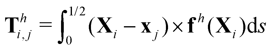 is the hydrodynamic torque generated by the i-th link about the left end of the j-th link (xj), and Te = −KΔθez is the elastic torque from the torsional spring. With the kinematic constraints x2 = x1 + (cos
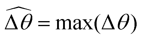 . Therefore, understanding the effect of shear-thinning rheology on elastohydrodynamic propulsion can be reduced to elucidating how
  are modified in a shear-thinning fluid in various scenarios.
 and compare the results with that for a continuous filament in Fig. 2.
 ) and hence the propulsion speed of a two-link swimmer. At large M, due to the dominance of the magnetic actuation on the dynamics of the actuated link, reduced viscous torques in a shear-thinning fluid has little influence on the actuation angle
  in a shear-thinning fluid [inset, Fig. 4(b)]. As Cu increases, the shear-thinning viscosity reduces the viscous torque; a smaller elastic torque is thus required to balance the viscous torque, leading to a reduced amplitude of the relative angle
  . The effect is analogous to a further increase in the spring constant K. The two-link swimmer hence behaves increasingly more like a rigid rod in a shear-thinning fluid as Cu increases [Fig. 4(c), K = 0.1], which acts to hinder propulsion. The same mechanism contributes to the decrease in propulsion speed for a continuous filament at high M [Fig. 2(a)], where shear-thinning rheology reduces the deformation along the filament owing to the reduced viscous forces [see Fig. 2(a) and (b)]. As a remark, even without any shape changes, an undulatory swimmer with the same gaits can swim slower in a shear-thinning fluid, because thrust is reduced to a larger extent than drag for undulatory swimmers.61 This latter effect combines with the effect due to gait changes to significantly reduce the propulsion performance at larger values of K in Fig. 4(a) [or smaller values of Sp in Fig. 2(a)]. On the other hand, at smaller values of K (e.g., K = 0.01), propulsion is relatively ineffective in the Newtonian limit due to the dominance of the viscous effect over the elastic effect on the dynamics of link 1. In this regime, the reduction in the viscous effect caused by shear-thinning rheology indeed allows more effective swimming gaits to emerge (the effect is analogous to an increased K). The two mechanisms, which act in tandem to hinder propulsion at large K, now counter-act and lead to less significant changes in the overall propulsion performance in the small K (or large Sp) regime.

 insets) as a function of K at varying Cu. (c) and (f) The shape of the swimmer over one actuation period T = 2π at equal time intervals (T/4) in Newtonian and shear-thinning fluids at different K; the intensity of the color increases as time advances.
 . Shear-thinning rheology generally reduces
  because a smaller elastic torque is required to balance the reduced viscous torque in a shear-thinning fluid. At higher values of K, a reduced
  makes the two-link swimmer behave more like a rigid rod with hindered propulsion performance. On the other hand, at smaller values of K, a reduced
  could act to enhance propulsion by allowing the two-link swimmer to deviate from relatively ineffective gaits in a Newtonian fluid in this regime. Overall, while these gait changes induced by shear-thinning rheology affect propulsion, we also note that, even without inducing any gait changes, shear-thinning rheology can also hinder the propulsion of undulatory swimmers by reducing the thrust more than drag.61 This later effect can act in tandem or counter-act with the effect due to gait changes to enhance or hinder propulsion by varying extents in different physical regimes. Taken together, the physical picture presented here captures qualitatively the behaviors observed for a continuous filament.