Enhancing drinking water quality modeling: leveraging physics informed neural networks for learning with imperfect reaction models and partial data
Received
22nd July 2025
, Accepted 4th September 2025
First published on 10th September 2025
Abstract
Chemical kinetics models, typically formulated as systems of ordinary or partial differential equations, are valuable tools for simulating drinking water quality. However, these models often face inaccuracies due to discrepancies between the laboratory and the real-world conditions, as well as limitations in experimental analytical methods, hindering the accurate representation of the true underlying chemical mechanisms. In this study, we propose a physics informed neural network (PINN), using the eXtreme Theory of Functional Connections, to improve the prediction of chemical concentrations over time. The PINN method accounts for imperfect chemical models and incorporates partial data to improve predictions. Focusing on reactions describing water disinfection residual and disinfectant byproduct formation, which are crucial for public health and regulatory compliance, we demonstrate that the PINN model is able to accurately predict the concentrations of chemical species across various pH values. Notably, the model extends its accuracy to predict concentrations of chemical species not originally included in its training data. The developed method can be extended to a variety of chemical systems, offering a wide array of potential applications.
Water impact
This work proposes a hybrid chemical and data-driven modeling approach to improve predictions of disinfection decay and byproduct formation in drinking water across varying pH levels. The proposed PINN-based method with the X-TFC technique integrates imperfect chemical models and incomplete data to enhance the accuracy of chemical concentration predictions.
|
1. Introduction
Chemical kinetics models play a crucial role in predicting chemical reactions relevant to drinking water quality in distribution systems.1 These models are typically described by systems of ordinary differential equations (ODEs). For example, chemical kinetics models that characterize chlorine decay,2 the formation of disinfection byproducts,3,4 and the fate of monochloramine5 are instrumental in the proper management of drinking water systems and prevent pathogen growth.6,7 Their importance is underscored by the persistent occurrence of health-based drinking water quality violations across the United States.8–10 Although chemical models are valuable tools for describing and predicting chemical concentrations in environmental systems, their accuracy can be limited. Even when developed using advanced analytical and experimental methods, the true underlying mechanisms may remain partially unknown or oversimplified.11 Moreover, these models are typically developed under controlled laboratory conditions, whereas real-world environmental systems introduce additional complexities that can lead to discrepancies between observed concentrations and model predictions.12 For instance, recent work to extend a monochloramine decay model to include N-nitrosodimethylamine (NDMA), a carcinogenic disinfection byproduct, illustrates these challenges as notable mismatches with experimental data remained despite advances in mechanistic understanding.5,11,13
Many approaches have been proposed to improve chemical kinetics models. Traditional calibration methods often rely on optimization to adjust rate constants based on measurements,14 but they often assume that all influential reactions are accounted for, which may not hold true. Alternatively, data-driven methods replace the process-based models with purely data-driven approaches, such as neural networks, to model drinking water quality, including chlorine residual and disinfection byproduct formation.12,15–20 However, data-driven approaches require extensive datasets, which are often difficult to collect and are typically incomplete or noisy, necessitating substantial pre-processing.19–21 These models tend to overfit to training data, leading to suboptimal performance outside their development domain.22
To address the limitations of relying solely on chemical or data-driven models, we propose a hybrid approach that incorporates both imperfect chemical models and partial data to improve predictions. Our methodology uses a physics-informed neural network (PINN), a novel framework that is gaining popularity across a range of scientific domains.23–25 The main idea behind PINNs is to leverage both process-based knowledge and data to enable more accurate and robust predictions, particularly in scenarios where physical models or sparse measurements alone are insufficient.26–28
Despite the growing use of PINN techniques across various scientific domains,29 several key limitations hinder their application to chemical kinetics in drinking water. These include (i) difficulty handling stiff equations, (ii) the use of PINNs primarily as numerical solvers rather than predictive tools, and (iii) reliance on time alone as an input. The first limitation stems from the inherent challenge of solving stiff ODEs, which are common in drinking water reaction processes.30–32 These systems are characterized by sharp gradients in the solution33 and pose difficulties for explicit numerical methods, often requiring extremely small timesteps or failing to converge altogether.34,35 Various methods have been proposed to improve the performance and reliability of PINNs, especially for stiff systems. These include techniques for enhancing physical fidelity by enforcing conservation laws,36,37 embedding domain-specific knowledge into the model structure,38 or adaptively balancing multiple loss components to address scale differences.39,40 Some studies have also proposed methods to reduce stiffness or improve training stability through quasi-steady-state assumptions or variable rescaling within the PINN framework.31,32 Other approaches focus on improving computational efficiency through tools for automatic differentiation41,42 or through neural ODE-based architectures designed to accelerate learning and simulation of chemical kinetics.43,44 The second limitation is that most current PINN implementations in chemical kinetics focus on solving governing equations without incorporating data to improve predictive performance,33 reducing their usefulness in settings where partial data is available. Finally, many implementations rely exclusively on time as an input while keeping all other parameters fixed;33 however, reaction rates in water systems are strongly influenced by other chemical characteristics, such as pH, which are essential for accurate modeling.5
To address these challenges, we propose a PINN-based method that integrates both imperfect chemical models and partial data to improve predictive performance. Specifically, we: (i) utilize the eXtreme Theory of Functional Connections (X-TFC) technique to model stiff chemical kinetics, aiming to improve accuracy and overcome limitations of previous technique. The X-TFC technique has demonstrated strong performance in rapidly and accurately solving various ODEs, including stiff chemical systems;33,45 (ii) enhance the X-TFC technique by transforming it into a predictive tool for chemical concentrations, integrating data and incorporating time and pH as input parameters into the training process; and (iii) demonstrate the performance of the proposed technique using three chemical models of increasing complexity for secondary disinfectant residuals in drinking water systems: a simplified model for monochloramine decay,5 an expanded monochloramine decay model accounting for natural organic matter,5,46 and a model for the formation of NDMA, a carcinogenic disinfection byproduct.11 We verify the approach using both simulated and experimental data. This integrated method, combining data and chemical modeling, can be extended to other chemical reactions and holds significant potential for improving public health through more accurate water quality predictions.
2. Methods
In this section, we first provide a brief overview of the X-TFC method for solving ODEs. We then present our proposed approach, including the formulation of the PINN model and the construction of loss functions for both chemical kinetics and data. Lastly, we describe the three chemical processes used to demonstrate the method.
2.1. Overview of X-TFC for solving first-order ODEs
We first illustrate the key features and intuition of the X-TFC method using a general nonlinear first-order ODE with an initial condition, representing a typical chemical reaction. Consider the following equation:| | 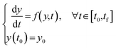 | (1) |
where y(t) is the concentration of a chemical species at time t, t0 is the initial time, tf is the final time, and y0 and f(y,t) are the initial concentration and the rate expression of a chemical species, respectively.
The X-TFC method has two unique features that make it an effective framework for solving stiff ODE systems compared to other PINN approaches: (i) it analytically satisfies initial conditions by reformulating the ODEs rather than relying on loss terms, and (ii) its choice of free function and training method enables high computational efficiency. First, unlike most methods that enforce both the initial condition and the rate of change of y(t) through loss functions during training,30,31 X-TFC satisfies the initial condition analytically using a constrained expression. This is achieved by incorporating the initial condition, y(t0), into the constrained formulation y(t) ≃ yCE(t) = g(t) + (y0 − g0), where g(t) is a free function defined on a the time domain and satisfies g(t) = g0. In our case, g(t) is represented by a shallow neural network (NN), as described below. This formulation ensures that yCE(t) satisfies the initial condition exactly. Substituting this constrained expression into the original ODE transforms it into an unconstrained problem, greatly simplifying the solution process. Second, X-TFC trains extremely quickly due to its choice of free function, g(t), which optimally approximates y(t). While the free function can be any real function on the simulation domain,45 prior studies have used deep NNs (Deep-TFC47), Chebyshev polynomials (CSVM48), and eXtreme learning machines (X-TFC49). In the X-TFC implementation, g(t) is a shallow, fully connected NN with one hidden layer trained using the extreme learning machine (ELM) method.33 ELM fixes input weights and biases randomly and tunes only the output weights, enabling fast training via iterative least squares regression. This makes it significantly more efficient than traditional backpropagation methods.50 To solve the ODE, the new unconstrained form,  is incorporated into the X-TFC framework via a loss function,
  , which quantifies the discrepancy between both sides of the equation. The model iteratively minimizes
  until convergence, ensuring the solution satisfies the original ODE and the initial condition. Further details and the application of this approach in our chemical kinetics modeling context are described next.
2.2. Extended X-TFC framework with data and pH integration
This section presents the proposed approach that improves the predictive capability of the X-TFC method by integrating data into the training process and incorporating pH as an additional input. As a key variable influencing many aquatic chemical reactions (particularly those that are acid-catalyzed or involve acid–base equilibria), pH enables the model to predict species concentrations at values beyond those used in training (see Text S1 in the SI for additional context). An overview of the main steps is shown in Fig. 1 and described in detail in the following subsections.
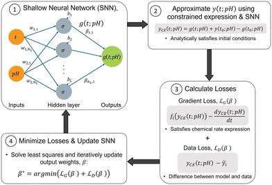 |
| | Fig. 1 Schematic of the proposed X-TFC PINN for water quality prediction. | |
2.2.1. Formulating the constrained expression.
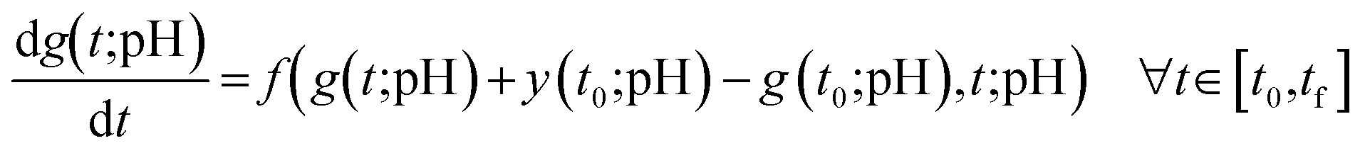
The system of ordinary differential equations describing chemical kinetics for multiple species as a function of time and pH is given by:| | 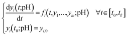 | (2) |
where i = 1,…, m is the species, yi(t;pH) is the concentration of a chemical species i at time t and given pH, t0 is the initial time, tf is the final time, and yi,0 and fi(t,y1,…, ym;pH) are the initial condition and the rate expression of a chemical species i, respectively. The chemical models and species used in this work are detailed in section 2.3.
After inclusion of pH, for each species and pH, the modified constrained expression is defined as follows:
| | | yCE(t;pH) = g(t;pH) + y(t0;pH) − g(t0;pH) | (3) |
Substituting the constrained expression and the free function, we get a new ODE that depends only on t and the free function g(t;pH):
| | 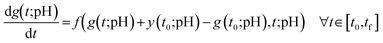 | (4) |
The next step is to identify, for each species, a free function, g(t;pH) that optimally approximates y(t;pH). The following subsections describe the extended X-TFC model components used to solve this general formulation, and detailed examples are provided in Texts S2–S5 in the SI.
2.2.2. Domain scaling.
Prior to setting up the X-TFC model, the t and pH domains are scaled into a standardized domain, x ∈ [x0, xf], which is independent of the underlying problem. This scaling process, typically used with x ∈ [0, 1] or x ∈ [−1, 1], achieves uniformity and better training accuracy.33 In this context, t ∈ [t0, tf] is mapped into x1 ∈ [x1,0, x1,f] using linear transformation, as follows:| | | x1 = x1,0 + c1(t − t0) | (5) |
where c1 is the mapping coefficient defined as:| |  | (6) |
Similarly, pH ∈ [pH0, pHf] is mapped into x2 ∈ [x2,0, x2,f]. The model is trained on the values in the standardized domain, discretized into Nt × NpH uniformly spaced training points. Accounting for mapping t and pH into a standardized domain, the constrained expression is reformulated as follows:
| | | yCE(x1; x2) = g(x1; x2) + y(x1,0; x2) − g(x1,0; x2) | (7) |
2.2.3. Neural network setup.
The free function is represented using a shallow NN, defined as:| |  | (8) |
where NL is the number of neurons, wj, βj, bj ∈ ![[Doublestruck R]](https://www.rsc.org/images/entities/char_e175.gif) are the input weight, output weight, and biases, respectively, corresponding to the jth neuron. w1j is the weight between x1, and neuron j, and w2j is the weight between x2, and neuron j. The activation function, σj(·), and number of neurons, NL, are selected by the user. We adopted the hyperbolic tangent function (tanh) as the activation function because its effectiveness in modeling still chemical kinetics.33 The input weights and biases are sampled from a random uniform distribution in the interval [−1, 1], leaving only β values to be tuned during model training. The coefficients β govern the NN's approximation of chemical concentrations. To identify the optimal values, the NN is trained using a gradient loss function,
are the input weight, output weight, and biases, respectively, corresponding to the jth neuron. w1j is the weight between x1, and neuron j, and w2j is the weight between x2, and neuron j. The activation function, σj(·), and number of neurons, NL, are selected by the user. We adopted the hyperbolic tangent function (tanh) as the activation function because its effectiveness in modeling still chemical kinetics.33 The input weights and biases are sampled from a random uniform distribution in the interval [−1, 1], leaving only β values to be tuned during model training. The coefficients β govern the NN's approximation of chemical concentrations. To identify the optimal values, the NN is trained using a gradient loss function,  , which minimizes the mismatch between the time derivatives and the governing equations, and a data loss function,
  , which accounts for discrepancies between predictions and available data.
2.2.4. Formulating the gradient loss function.
The ODE problem consists of two components: the initial value and the rate of change with respect to time. The initial value is enforced through the constrained expression in eqn (7), while the rate of change is incorporated into the loss function minimized during training. For each chemical species and training point, the gradient loss  quantifies the discrepancy between the time derivative and the governing function, i.e., the left- and right-hand sides of eqn (4), where the free function g(t;pH) is represented by the shallow NN given in eqn (8). To derive the gradient loss expression, the first-order derivative of eqn (8) with respect to time is:
| |  | (9) |
Higher order derivatives can also be derived using the chain rule.33 Substituting the constrained expression and its derivative into the gradient loss function yields:
| |  | (10) |
where
σi,j are the activation functions evaluated at the (
i,
j) training points, and
σ0 corresponds to the initial conditions. Minimizing the loss function for each captures the concentration dynamics defined by the chemical model.
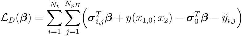
2.2.5. Formulating the data loss function.
An additional data loss term is included to incorporate available data. For a specific species, this is achieved by minimizing the deviation between the available data, ỹi,j, at point (i, j) and the NN prediction:| |  | (11) |
We note that training requires extremely fine time intervals (on the order of 10−5 seconds), which is typically impractical for many laboratory or field settings and the sampled data rarely align with the model's grid. In section 3.3, we show how this challenge can be addressed by interpolating the available data, e.g., using regression or cubic splines, and evaluating it at the required training points.51,52
2.2.6. Minimizing the loss functions.
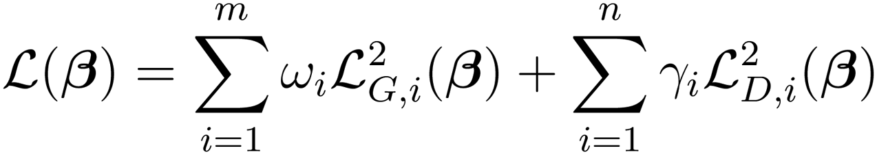
Minimizing the gradient and data loss functions involves solving an unconstrained non-linear optimization problem,| |  | (12) |
where m is the number of species, n is the number of species for which data is available, ωi is a user-defined weight applied to the loss function for each species in the chemical model, and γi is a user-defined weight for each species with a data loss term. This optimization problem can be solved using non-linear least squares, such as those based on the Gauss–Newton algorithm.33,53 In each iteration, k, the loss functions are approximated using a linear function, and the output weights, β, are updated as βk+1 = βk + sΔβk, and s is the user-defined learning rate. The Δβ are calculated as follows:| |  | (13) |
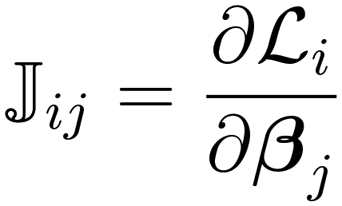
where ![[Doublestruck J]](https://www.rsc.org/images/entities/char_e16d.gif) is the Jacobian matrix of the loss functions calculated as:
is the Jacobian matrix of the loss functions calculated as:| |  | (14) |
The iterations continue until either the L2 norm of the loss functions or the difference in the L2 norm between consecutive iterations falls below a user-defined tolerance, ε.33 Further details on the choice of hyperparameters are included in the SI.
2.2.7. Time subdomains.
Due to the stiffness of the differential equations, X-TFC may result in inaccurate solutions when implemented over a long time domain.33,45 In order to improve the solution accuracy, the entire time domain is split into n = 1,…, NT logarithmic-spaced subdomains, consisting of a separate X-TFC model in each subdomain. In the first subdomain, the initial concentration of each species is specified by the initial conditions of the ODEs. In the subsequent subdomains, the initial concentration of each species is set equal to the final concentration of the previous subdomain,  . The solution over the entire time domain is achieved by concatenating the solutions from each subdomain.
2.3. Chemical kinetics process models
We demonstrate our proposed approach applied to model monochloramine decay, its interaction with natural organic matter,46 and its association with the formation of reactive nitrogen species.11,54 All three processes involve bulk-phase reactions occurring within the water column. We verify the approach using both simulated and experimental data. Monochloramine is used as a secondary disinfectant to maintain a chlorine residual within a distribution system by approximately 25% of water utilities in the United States,55 highlighting the need for accurate modeling. The associated chemical processes involve stiff systems of differential equations, driven by sharp gradients and large concentration differences among species,5,11,46 making them a compelling test case for the proposed PINN framework. The three chemical processes are outlined below, with additional details provided in the SI.
2.3.1. Simplified monochloramine decay.
The chemical kinetics model describing abiotic decay of monochloramine was originally proposed in 1992 as the unified model, comprising a set of 14 reactions.5 The reactions of the unified model are detailed in Table S1 in the SI (reactions r1–r14). The first chemical kinetics process (CKP1) model utilized in this study consists of four species and three chemical reactions (r1–r3), forming a subset of the unified model. The four species included in CKP1 are TOTNH (total concentration of ammonia and ammonium), TOTCl (total amount of hypochlorous acid and hypochlorite), monochloramine (NH2Cl), and dichloramine (NHCl2). Additional details of acid/base chemistry relevant to the speciation of TOTNH and TOTCl based on pH are included in Text 1 in the SI. We initially utilize this model for demonstration purposes, as it contains three of the primary equations and species governing the monochloramine decay process. Specifically, these reactions describe the formation of monochloramine from hypochlorous acid and ammonia, as well as the formation of dichloramine from monochloramine and hypochlorous acid.5 The PINN model for CKP1, including the ODE system of equations, constrained expressions, loss functions, and Jacobian, are detailed in Text S2 in the SI.
2.3.2. Monochloramine decay in the presence of natural organic matter.
In 2005, the unified model was expanded by introducing two additional reactions to account for the impact of dissolved organic carbon (DOC).46 The interaction between monochloramine and DOC is important because monochloramine undergoes rapid initial decay within approximately 10 hours of the reaction. This set of 16 reactions has gained widespread acceptance and is extensively used for simulating monochloramine decay in water distribution systems.6,56 We utilize the expanded model as our second chemical kinetic process (CKP2). CKP2 consists of the unified model for monochloramine decay (reactions 1–14 in Table S1 in the SI) and two additional reactions (reactions 15–16 in Table S1 in the SI) describing interactions with fast and slow components of DOC with monochloamine and hypochlorous acid.5,46 In addition to the four species previously defined, TOTCl, TOTNH, NH2Cl, and NHCl2, CKP2 models an unidentified intermediate species (I), trichloramine (NCl3), DOC1 and DOC2. DOC1 represents the fast-reacting portion of DOC, which is responsible for the initial fast decay of NH2Cl (described in r15 in Table S1). DOC2 represents the slow-reacting portion of DOC, which reacts with hypochlorous acid and increases the rate of monochloramine decay throughout the duration of the reaction. Details for the X-TFC model for CKP2 are included in Text S3 in the SI.
2.3.3. Monochloramine decay and formation of reactive nitrogen species.
In the third chemical kinetic process (CKP3) model, we leverage recent research advancement focused on identifying reactions and pathways associated with the formation of disinfection byproduct resulting from monochloramine degradation.11,54 In constructing the PINN model for CKP3, we utilized an expanded version of the unified model, recently proposed to incorporate pathways for the formation of reactive nitrogen species (RNS). This model specifically addresses NDMA, a carcinogenic byproduct of drinking water disinfection.11 CKP3 consists of the unified and reactive nitrogen species model (UN-RNS) for chloramine decay and NDMA formation proposed in ref. 11. The UN-RNS model contains 143 reactions, of which 114 reactions describe the decay of peroxynitrous acid and peroxynitrite.57 To simplify the implementation in X-TFC without compromising accuracy, we approximated the 114 reactions with a single calibrated first-order reaction across pH values 7–10, ensuring concentration agreement of peroxynitrous acid and peroxynitrite between the full and the surrogate UN-RNS models. This simplification is supported by a sensitivity analysis in ref. 57, which identified the dominant reaction as the first-order decay of peroxynitrous acid to nitric acid. The final UN-RNS model used here consists of 30 reactions and 15 chemical species. In addition to the model, we used experimental data reported in ref. 11.
3. Results
Our methodology was carried out in three phases. In phase 1, we used CKP1 and CKP2 to evaluate the modified X-TFC model trained solely on chemical reactions of increasing complexity, without additional data. In phase 2, we trained the model using a combination of inaccurate reactions and partial data, available for only a subset of species. In phase 3, we applied the methodology to CKP3, involving a more complex and inaccurate chemical model along with partial experimental data.11 Prediction accuracy was assessed for in-sample pH (used in training), out-of-sample pH (excluded from training), and holdout species (not included in the training data). Model error was computed using two complementary metrics: weighted root mean squared error (WRMSE) and weighted absolute percentage error (WAPE). These metrics are commonly employed in machine learning to account for varying importance or scale of data points.58,59 A full mathematical description and error values are provided in Text S6 and Tables S2–S4 in the SI. In the results below, we use an initial monochloramine (NH2Cl) concentration of 4.22 × 10⁵ mol l−1 (equivalent to 3.0 mg l−1 as Cl2) for CKP1 and CKP2, consistent with typical values found in water treatment plant effluent entering distribution systems.60–62 For CKP3, we adopt the initial concentrations reported in the experimental study.11 All results are compared against solutions obtained using ode15s, a MATLAB solver designed for stiff ODEs.63 The training times for all models range from 5 to 70 seconds, depending on the model, using a machine equipped with an Intel(R) Core(TM) i7-1165G7 CPU@2.80 GHz and 16 GB of RAM.
3.1. Phase 1: chemical reaction-based training and validation
3.1.1. In-sample pH training.
We first evaluate the X-TFC model's ability to estimate concentrations of four species over a 7 day period. The model is trained using only the chemical kinetics equations (excluding advection and diffusion) for CKP1 and CKP2 at in-sample pH values of 7, 8, 9, and 10. Fig. 2 and 3 present the results for CKP1 and CKP2, respectively, with solid lines showing X-TFC predictions and dashed lines representing solutions from ode15s. The close agreement between the two confirms the X-TFC model is effective in solving stiff ODEs with varying scales and sharp gradients at in-sample pH values. Details on the loss functions and hyperparameters are provided in Texts S2 and S3 of the SI.
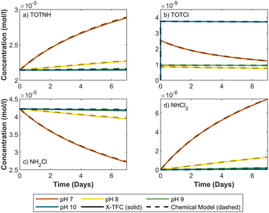 |
| | Fig. 2 CKP1 X-TFC results for in-sample pH values compared to chemical model solved using ode15s: a) TOTNH, b) TOTCl, c) NH2Cl, and d) NHCl2. X-TFC (solid lines), chemical model (dashed lines), different pH values (colored lines). | |
 |
| | Fig. 3 CKP2 X-TFC results for in-sample pH values compared to chemical model solved using ode15s: a) TOTNH, b) TOTCl, c) NH2Cl, d) NHCl2 e) I, f) DOC2, g) NCl3, and h) DOC1. X-TFC (solid lines), chemical model (dashed lines), different pH values (colored lines). Note that DOC1 does not vary with pH, hence the lines for different pH values overlap. | |
3.1.2. Out-of-sample pH validation.
To evaluate how well each X-TFC model is able to interpolate for out-of-sample pH values, we assessed the trained X-TFC model across pH 7.5, 8.5, and 9.5. Results for CKP1 and CKP2 are shown in Fig. 4 and 5. For CKP1, the X-TFC results closely matches the ode15s solution for TOTNH, NH2Cl, and NHCl2 (Fig. 4a, b and d). While the X-TFC result for TOTCl follows a similar trend, there is a difference in the predicted concentration. This is likely due to the rapid initial increase in TOTCl, which challenges the model's accuracy. Additionally, the TOTCl response is non-monotonic with respect to pH, i.e., it is highest at pH 10, followed by pH 7, 9, and 8, making interpolation difficult. We hypothesize that this irregular pH-response pattern contributes to the X-TFC model's reduced accuracy for out-of-sample pH values in this system.
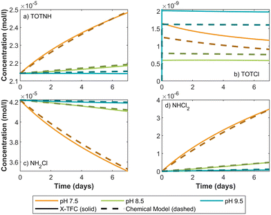 |
| | Fig. 4 CKP1 X-TFC results for out-of-sample pH values compared to chemical model using ode15s: a) TOTNH, b) TOTCl, c) NH2Cl, and d) NHCl2. X-TFC (solid lines), chemical model (dashed lines), different pH values (colored lines). | |
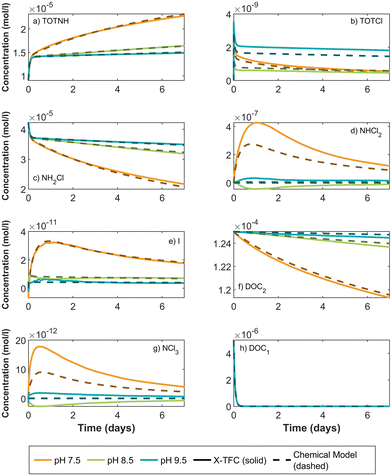 |
| | Fig. 5 CKP2 X-TFC results for out-of-sample pH values compared to chemical model solved using ode15s: a) TOTNH, b) TOTCl, c) NH2Cl, d) NHCl2 e) I, f) DOC2, g) NCl3, and h) DOC1. X-TFC (solid lines), chemical model (dashed lines), different pH values (colored lines). Note that DOC1 does not vary with pH, hence the lines for different pH values overlap. | |
Out-of-sample results for CKP2 also show good agreement with ode15s solutions for TOTNH, NH2Cl, I, DOC1 and DOC2 (Fig. 5a, c, e, f and h). However, NHCl2, NCl3, and I show negative chemical concentrations during parts of the prediction period. These values result from model error and do not reflect physically meaningful concentrations. Despite this, the model's performance for species I is considered strong, with negative values appearing only briefly at pH 7.5. For NHCl2 and NCl3, large differences in concentration magnitudes between training points, ranging from 10−6 to 10−8 for NHCl2 and 10−11 to 10−13 for NCl3, pose challenges for interpolation at pH 7.5 (see Fig. 3). In that case, the model slightly overpredicts peak values but still captures the correct trend and converges toward the ground truth over time. Similar deviations are observed at pH 8.5 and 9.5, though overall trends remain consistent with the true model.
3.2. Phase 2: integrating inaccurate chemical reactions with partial data
Our primary objectives are twofold: (i) to assess the X-TFC model's ability to compensate for inaccuracies in the chemical model by leveraging available data, and (ii) to evaluate its predictive accuracy for out-of-sample pH values and hold-out species for which no training data were provided. These challenges reflect real-world conditions, where chemical models may not capture all reaction dynamics and data are often available for only a subset of species.
3.2.1. Evaluation strategy.
To simulate such scenarios, we train the X-TFC model using inaccurate reactions and partial data limited to selected species. Here, training data refers to data used for in-sample pH values, and hold-out species are those for which no data was used during training. To ensure the model is not simply overfitting to in-sample data, we validate its performance on out-of-sample pH values using the same trained X-TFC model. Hold-out data refers to data excluded from training and used as ground truth for assessing prediction accuracy under these out-of-sample conditions.
For CKP1, training data was provided for TOTNH and TOTCl at in-sample pH values (7, 8, 9, and 10), while data for held-out species NH2Cl and NHCl2 was excluded. The chemical model results were generated by solving the chemical reactions described in section 2.3.1 using the ode15s solver. To simulate data with model inaccuracies, we generated the training data using increased rate constants, deviating from the original reaction kinetics. This generated data serves as the ground truth for evaluating the X-TFC model's performance. Details on model setup, loss functions, and hyperparameters are provided in Text 4 of the SI.
For CKP2, a more complex kinetic model, the X-TFC training used only the first 14 of 16 reactions, simulating incomplete mechanistic knowledge consistent with the state of understanding prior to 2005.46 The full 16-reaction system (section 2.3.2, Table S1) was used to generate ground truth data via ode15s. Training data were limited to TOTNH, TOTCl, and NH2Cl at in-sample pH values (7, 8, 9, and 10), with all other species treated as hold-out. Species DOC1 and DOC2 were omitted entirely, as they are products of the excluded reactions. Implementation details are provided in Text 5 of the SI.
3.2.2. CKP1 results.
The X-TFC model accurately predicts chemical concentrations across both in-sample and out-of-sample pH values, even for species excluded from training, demonstrating its ability to generalize beyond both data and model limitations. Fig. 6a, c and e show X-TFC predictions for in-sample pH values (7 and 8), while Fig. 6b, d and f show predictions for out-of-sample pH values (7.5 and 8.5). Results for pH 9, 9.5, and 10 are omitted for clarity. Solid lines represent X-TFC predictions; dotted lines indicate training data (black) and hold-out data (color), which serve as ground truth; and dashed lines represent the inaccurate chemical model.
 |
| | Fig. 6 CKP1 X-TFC results compared to chemical model, training data, hold-out data, and hold-out species. In-sample pH results: a) TOTNH, c) TOTCl and e) NH2Cl. Out-of-sample pH results: b) TOTNH, d) TOTCl and f) NH2Cl. X-TFC (solid lines), chemical model (dashed lines) training data (dotted, black), hold-out data and hold-out species (colored dotted lines), different pH values (colored lines). | |
For TOTNH and TOTCl, the X-TFC predictions match the training data for in-sample pH, demonstrating successful learning despite inaccuracies in the reaction model. Remarkably, X-TFC also accurately predicts concentrations of the hold-out species NH2Cl, even though no training data for this species were used. This underscores the model's ability to leverage partial data and mechanistic structure to infer missing species behavior. If X-TFC were purely data-driven, it could not predict NH2Cl concentrations. Conversely, relying solely on the inaccurate chemical model yields poor predictions for all species. The X-TFC model succeeds by integrating both imperfect chemical equations and partial data, correcting for model deficiencies and aligning closely with the ground truth. For out-of-sample pH, TOTNH and TOTCl predictions remain accurate, though a slight offset is observed for TOTCl, consistent with trends noted in section 3.1.2. Additional insights into NHCl2 predictions are discussed in section 4.
3.2.3. CKP2 results.
Consistent with previous results, the X-TFC model accurately predicts the concentrations of a hold-out species in a more complex chemical system, even without access to its training data. Fig. 7 illustrates this performance for the unidentified intermediate species I, which we include in the analysis since it is hypothesized to be HNO, a precursor to NDMA formation.11 This species was excluded from training but predicted accurately by the model for both in-sample and out-of-sample pH values. Solid lines indicate X-TFC predictions, dotted lines show hold-out data, and dashed lines represent the incomplete chemical model. Results for all other species in this system show similar accuracy and are included in Fig. S1–S5 of the SI.
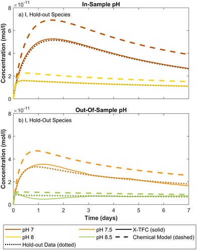 |
| | Fig. 7 CKP2 X-TFC results compared to chemical model and hold-out species I (unidentified intermediate): a) in-sample pH, b) out-of-sample pH. X-TFC (solid lines), chemical model (dashed lines), hold-out data (dotted lines), and different pH values (colored lines). | |
3.3. Phase 3: application to experimental data and a complex chemical system
To demonstrate the applicability of the X-TFC method to experimental data and a larger, more complex chemical system, we use the chemical reaction scheme and data from ref. 11. We trained two separate X-TFC models, each incorporating a different type of data. The first X-TFC model used experimental measurements from ref. 11, which reported concentrations for five species: NH2Cl, NHCl2, NDMA, N2O, and O2, at pH 7, 8, 9, and 10. While this dataset provides real kinetic observations, it lacks measurements for several species, limiting our ability to evaluate model performance on unmeasured (hold-out) species. Therefore, to overcome this limitation, a second X-TFC model was trained using simulated data generated from the same chemical model but with deliberately altered rate constants (reduced from those in ref. 11) to introduce model-data mismatch. This approach mirrors that used in CKP1 phase 2 and provides data for all species, enabling evaluation of model performance on hold-out species. Because X-TFC training requires extremely fine time intervals (on the order of 10−5 seconds), we interpolated the experimental measurements using cubic splines and regression methods51,52 to align them with the X-TFC grid. The interpolated curves used for training are shown in Fig. S6 of the SI.
In both models, X-TFC accurately reproduces the training data for the five measured species. Fig. 8 focuses on a hold-out species, TOTONOO (total peroxynitrite and peroxynitrous acid). In Fig. 8a, where simulated data was used, the X-TFC predictions closely match the hold-out data, outperforming the standalone chemical model (dashed line). In Fig. 8b, where experimental data was used, no hold-out data exists for TOTONOO. However, the model's success in the simulated case provides confidence in its predictions under the experimental setup as well. Additional analysis shows similarly strong performance for other hold-out species (e.g., HNO and NO−) in the simulated case, further supporting the ability of X-TFC to make reliable predictions even for species not included in training.
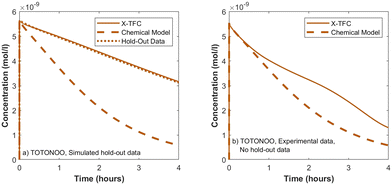 |
| | Fig. 8 CKP3 X-TFC results for TOTONOO species compared to chemical model and hold-out data at pH 8 using training data for NH2Cl, NHCl2, NDMA, O2 and N2O, species. a) Training and hold-out data generated by simulation and b) training data generated by laboratory experiments, no hold-out data exists for TOTONOO. | |
4. Discussion
4.1. Future directions
This study demonstrates the potential of the X-TFC framework for advancing PINNs in water quality modeling, experimental design, and public health protection, with key findings and future directions summarized below.
(i) Toward interpretability of PINN predictions.
In general, PINNs include some species with training data and others without. For species with data, predictions are shaped by both the data loss and the gradient loss, while for species without data, concentrations are inferred from the governing reactions and constrained species for which data is available. This framework shows not only which species are well constrained by data, but also how constraints propagate through reactions to unmeasured species, providing interpretability beyond simple curve fitting. Fig. 9 illustrates this for CKP1. X-TFC accurately predicts TOTNH and TOTCl, which are constrained by the data (Fig. 9a and b). The hold-out species NH2Cl follows the expected depletion trend (Fig. 9c), while NHCl2 is predicted lower than the chemical model (Fig. 9d). This is because NHCl2 depends on NH2Cl through the third reaction in CKP1 (Table S1 in the SI), and since X-TFC underpredicts NH2Cl relative to the chemical model, the resulting NHCl2 concentration is also underestimated. In this way, the X-TFC model demonstrates how including data for some species can propagate through the reactions, pointing to which processes and measurements most strongly affect the accuracy of others. Future work should build on this by developing systematic interpretability analyses, such as residual or gradient-based analysis, that can guide experimental design and identify the most critical species to measure.
 |
| | Fig. 9 X-TFC results for CKP1 compared to chemical model, training data, and hold-out species for pH 7. a) TOTNH, b) TOTCl, c) NH2Cl, and d) NHCl2. X-TFC (solid lines), chemical model (dashed lines) training data (dotted, black), hold-out species (colored dotted line). | |
(ii) Integrating with hydraulic models for system-wide water quality estimation.
When coupled with a calibrated hydraulic model, the X-TFC framework can support water quality estimation across drinking water distribution systems, capturing both bulk and wall reactions. Hydraulic models can estimate water age and pipe-specific conditions throughout the network.64 X-TFC models, trained to relate chemical concentrations to time and combined with pipe-specific conditions for wall reactions, can then use this information to estimate concentrations at any location. Although this integration introduces additional complexity, it enables more precise spatial and temporal mapping of water quality, particularly when X-TFC is trained on location-specific data.
(iii) Real-time application through digital twin integration.
The extremely short training time of X-TFC model (ranging from 5 to 70 seconds, depending on the model complexity), makes it well-suited for real-time applications.65 Utilizing near-real-time data from water quality sensors within the water distribution network, the X-TFC model could be continuously re-trained to obtain accurate predictions of water quality. This approach would complement other data assimilation techniques, such as a Kalman filters.66
(iv) Incorporating multiple parameters.
By including pH as an input variable, the X-TFC model supports predictions across a range of water quality conditions. This flexibility can be extended to incorporate other variables such as alkalinity or oxidation–reduction potential (ORP). As real-time sensors become increasingly widespread in distribution systems and premise plumbing,67,68 the ability to train PINNs on multiple input parameters will be essential. Due to the model's fast evaluation time, sensor outputs for pH, ORP, or other variables could be used in real time to continuously estimate concentrations of unmeasured chemical species.
(v) Improving predictions for emerging contaminants.
As water quality concerns intensify and chemical models continue to evolve, the X-TFC framework offers a promising path to correct model inaccuracies and improve predictions of key chemical species. For example, a chemical kinetics model was previously developed to describe the formation of brominated haloamines and other toxic brominated disinfection byproducts.69 Although the model generally aligned with experimental data, notable discrepancies remained. Given the expected growth in desalinated seawater use and the resulting risks of DBP formation,70 integrating the X-TFC PINN framework could substantially improve predictions of brominated species, informing the design and operation of drinking water infrastructure in regions with high bromine levels in source water.
4.2. Limitations and future work
There are several promising directions to advance the proposed X-TFC modeling framework, both in terms of algorithmic development and chemical modeling: (i) Hyperparameter tuning: the X-TFC model includes several hyperparameters (e.g., learning rate, loss weights, neurons, subintervals). In this study, tuning was manual but guided by chemical understanding, for example, giving higher weights to low-concentration species to better capture their dynamics. A more systematic sensitivity analysis (e.g., using KKT conditions or error propagation via MLE39,40) could improve both performance and reproducibility. (ii) Data adequacy and uncertainty quantification: as with any data-driven approach, performance depends on the quality and availability of data, and the method is not guaranteed to work under all conditions. A key advantage of PINNs is that they require substantially less data than purely data-driven methods because they combine process-based modeling with observations. For example, in section 3.4 (CKP3), when working with experimental data, interpolation (via regression or cubic splines) was a necessary first step to address sparsity and irregular sampling. Future work should explicitly quantify different sources of uncertainty, such as measurement noise, limited data, and process, and assess their relative contribution to overall PINN performance.71 (iii) Random seed dependence: model performance showed sensitivity to the random seed, likely due to the initialization of weights and biases. Prior work72 demonstrated that initializing weights to enhance variability across the activation domain improves model robustness. However, their method is limited to single-input models. Future research should explore initialization strategies that promote activation diversity in multi-input settings. (iv) Optimization strategy: we employed a Gauss–Newton based method for minimizing the X-TFC loss functions. Future work could explore alternative optimizers, including Adam,73 L-BFGS,74 and second-order methods,75 to improve convergence speed and predictive performance. (iv) Gradient computation: this study manually derived and applied analytical gradients to ensure transparency and reduce overhead. Future implementations could benefit from automatic differentiation tools provided by frameworks such as Autograd41 and JAX,42 which offer greater flexibility and ease of use. (v) Dynamic pH conditions: we assumed a well-buffered system with constant pH, but in real applications, pH may vary over time. Future implementations could allow time-varying pH either by adjusting it across time subintervals or by modeling hydrogen ion dynamics explicitly within the reaction network. (vi) Application to other chemical systems: while this study focused on monochloramine decay and NDMA formation, the X-TFC framework should also be evaluated on other chemical processes, such as free chlorine,76 trihalomethane formation,3 nitrification in distribution systems,77 and bromine haloamine formation,69 to assess its generalizability across diverse water quality contexts.
5. Conclusions
Chemical kinetic models are essential tools for simulating the formation and decay of chemical species in drinking water distribution systems. However, their accuracy is often limited by incomplete knowledge of reaction dynamics. This study presents a PINN framework based on the X-TFC methodology that integrates partial empirical data with imperfect chemical models, enabling improved modeling of stiff chemical kinetics. We demonstrated the effectiveness of this approach across three chemical reaction schemes of increasing complexity, all relevant to monochloramine decay and the formation of NDMA, a carcinogenic byproduct of water disinfection. Our results show that the X-TFC model can accurately predict chemical concentrations, even for species excluded from training, with computation times on the order of seconds to minutes. This makes the approach especially promising for real-time or system-wide water quality assessments. Beyond water systems, the framework offers potential for other domains characterized by stiff ODEs and partial observations, such as atmospheric chemistry78 and systems biology,79 highlighting its broad applicability across environmental and biological sciences.
Author contributions
Matthew Frankel: conceptualization, methodology, software, formal analysis, writing – original draft. Mario De Florio: methodology, software, writing – review & editing. Enrico Schiassi: methodology, software, writing – review & editing. Lynn E. Katz: writing – review & editing. Kerry Kinney: writing – review & editing. Charles J. Werth: writing – review & editing. Corwin Zigler: writing – review & editing. Lina Sela: conceptualization, methodology, writing – review & editing, supervision, funding acquisition.
Conflicts of interest
There are no conflicts to declare.
Data availability
Supplementary information is available. See DOI: https://doi.org/10.1039/D5EW00682A.
SI includes additional details on impact of pH on chemical systems, mathematical details on each PINN model, additional model results, model error metrics, and data interpolation results. Example code used to generate results available at https://github.com/mfrankel923/Chemical-Data-X-TFC.
Acknowledgements
This work was supported by the National Science Foundation under Grant 1953206. The authors acknowledge Dr. Julian Fairey, Dr. David Wahman, and Dr. Huong Pham for discussions during the framing of this study, and for sharing the data from their previous experimental work.
References
- S. Hossain, C. W. K. Chow, D. Cook, E. Sawade and G. A. Hewa, Review of chloramine decay models in drinking water system, Environ. Sci.: Water Res. Technol., 2022, 8, 926–948, 10.1039/D1EW00640A.
- J. Powell, J. West, N. Hallam, C. Forester and J. Simms, Performance of various kinetic models for chlorine decay, J. Water Resour. Plan. Manage., 2000, 126, 13–20, DOI:10.1061/(ASCE)0733-9496(2000)126:1(13).
- A. Abokifa, J. Yang, C. Lo and P. Biswas, Investigating the role of biofilms in trihalomethane formation in water distribution systems with a multicomponent model, Water Res., 2016, 104, 208–219, DOI:10.1016/j.watres.2016.08.006.
- D. Hogue, P. B. Mirchandani and T. H. Boyer, Predictive capability of thm models for drinking water treatment and distribution, Environ. Sci.: Water Res. Technol., 2023, 9, 2745–2759, 10.1039/D3EW00308F.
- C. T. Jafvert and R. L. Valentine, Reaction scheme for the chlorination of ammoniacal water, Environ. Sci. Technol., 1992, 26(3), 557–586, DOI:10.1021/es00027a022.
- D. G. Wahman, Web-based applications to simulate drinking water inorganic chloramine chemistry, J. - Am. Water Works Assoc., 2018, 110, E43–E61, DOI:10.1002/awwa.1146.
- S. Hossain, C. W. Chow, D. Cook, E. Sawade and G. A. Hewa, Review of chloramine decay models in drinking water system, Environ. Sci.: Water Res. Technol., 2022, 8(5), 926–948 RSC.
- B. R. Scanlon, S. Fakhreddine, R. C. Reedy, Q. Yang and J. G. Malito, Drivers of spatiotemporal variability in drinking water quality in the united states, Environ. Sci. Technol., 2022, 56(18), 12965–12974, DOI:10.1021/acs.est.1c08697.
- S. Michielssen, M. C. Vedrin and S. D. Guikema, Trends in microbiological drinking water quality violations across the united states, Environ. Sci.: Water Res. Technol., 2020, 6, 3091–3105, 10.1039/D0EW00710B.
- M. Allaire, H. Wu and U. Lall, National trends in drinking water quality violations, Proc. Natl. Acad. Sci. U. S. A., 2018, 115(9), 2078–2083, DOI:10.1073/pnas.1719805115.
- H. T. Pham, D. G. Wahman and J. L. Fairey, Updated reaction pathway for dichloramine decomposition: Formation of reactive nitrogen species and n-nitrosodimethylamine, Environ. Sci. Technol., 2021, 55(3), 1740–1749, DOI:10.1021/acs.est.0c06456.
- M. De Santi, U. T. Khan, M. Arnold, J.-F. Fesselet and S. I. Ali, Forecasting point-of-consumption chlorine residual in refugee settlements using ensembles of artificial neural networks, npj Clean Water, 2021, 4, 35, DOI:10.1038/s41545-021-00125-2.
- M. Sgroi, F. G. Vagliasindi, S. A. Snyder and P. Roccaro, N-nitrosodimethylamine (ndma) and its precursors in water and wastewater: A review on formation and removal, Chemosphere, 2018, 191, 685–703, DOI:10.1016/j.chemosphere.2017.10.089.
- S. I. Ali, S. S. Ali and J.-F. Fesselet, Evidence-based chlorination targets for household water safety in humanitarian settings: recommendations from a multi-site study in refugee camps in south sudan, jordan, and rwanda, Water Res., 2021, 189, 116642, DOI:10.1016/j.watres.2020.116642.
- A. A. Ahmed, S. Sayed, A. Abdoulhalik, S. Moutari and L. Oyedele, Applications of machine learning to water resources management: A review of present status and future opportunities, J. Cleaner Prod., 2024, 140715, DOI:10.1016/j.jclepro.2024.140715.
- A. Riyadh, A. Zayat, A. Chaaban and N. M. Peleato, Improving chlorine residual predictions in water distribution systems using recurrent neural networks, Environ. Sci.: Water Res. Technol., 2024, 10(10), 2533–2545, 10.1039/D4EW00329B.
- D. W. Dunnington, B. F. Trueman, W. J. Raseman, L. E. Anderson and G. A. Gagnon, Comparing the predictive performance, interpretability, and accessibility of machine learning and physically based models for water treatment, ACS ES&T Eng., 2020, 1, 348–356, DOI:10.1021/acsestengg.0c00053.
- S. Soyupak, H. Kilic, I. Karadirek and H. Muhammetoglu, On the usage of artificial neural networks in chlorine control applications for water distribution networks with high quality water, J. Water Supply: Res. Technol.--AQUA, 2011, 60, 51–60, DOI:10.2166/aqua.2011.086.
- M. J. Kennedy, A. H. Gandomi and C. M. Miller, Coagulation modeling using artificial neural networks to predict both turbidity and dom-parafac component removal, Journal of Environmental, Chem. Eng., 2015, 3, 2829–2838, DOI:10.1016/j.jece.2015.10.010.
- G. Hu, H. R. Mian, S. Mohammadiun, M. J. Rodriguez, K. Hewage and R. Sadiq, Appraisal of machine learning techniques for predicting emerging disinfection byproducts in small water distribution networks, J. Hazard. Mater., 2023, 446, 130633, DOI:10.1016/j.jhazmat.2022.130633.
- A. El Bilali, H. Lamane, A. Taleb and A. Nafii, A framework based on multivariate distribution-based virtual sample generation and dnn for predicting water quality with small data, J. Cleaner Prod., 2022, 368, 133227, DOI:10.1016/j.jclepro.2022.133227.
- A. Aliashrafi, Y. Zhang, H. Groenewegen and N. M. Peleato, A review of data-driven modelling in drinking water treatment, Rev. Environ. Sci. Bio/Technol., 2021, 1–25, DOI:10.1007/s11157-021-09592-y.
- J. Ye, N. C. Do, W. Zeng and M. Lambert, Physics-informed neural networks for hydraulic transient analysis in pipeline systems, Water Res., 2022, 221, 118828, DOI:10.1016/j.watres.2022.118828.
- M. Sarabian, H. Babaee and K. Laksari, Physics-informed neural networks for brain hemodynamic predictions using medical imaging, IEEE Trans. Med. Imaging, 2022, 41(9), 2285–2303, DOI:10.1109/TMI.2022.3161653.
- K. Shukla, P. C. Di Leoni, J. Blackshire, D. Sparkman and G. E. Karniadakis, Physics-informed neural network for ultrasound nondestructive quantification of surface breaking cracks, J. Nondestruct. Eval., 2020, 39, 1–20, DOI:10.1007/s10921-020-00705-1.
-
M. Raissi, P. Perdikaris and G. E. Karniadakis, Physics informed deep learning (part I): Data-driven solutions of nonlinear partial differential equations, arXiv, 2017, preprint, arXiv:1711.10561, DOI:10.48550/arXiv.1711.10561.
-
M. Raissi, P. Perdikaris and G. E. Karniadakis, Physics informed deep learning (part ii): Data-driven discovery of nonlinear partial differential equations, arXiv, 2017, preprint, arXiv:1711.10566, DOI:10.48550/arXiv.1711.10566.
- G. E. Karniadakis, I. G. Kevrekidis, L. Lu, P. Perdikaris, S. Wang and L. Yang, Physics-informed machine learning, Nat. Rev. Phys., 2021, 3, 422–440, DOI:10.1038/s42254-021-00314-5.
- S. Cuomo, V. S. di Cola, F. Giampaolo, G. Rozza, M. Raissi and F. Piccialli, Scientific machine learning through physics-informed neural networks: Where we are and what's next, J. Sci. Comput., 2022, 92(88), 1–62, DOI:10.1007/s10915-022-01939-z.
- S. Wang, Y. Teng and P. Perdikaris, Understanding and mitigating gradient pathologies in physics-informed neural networks, SIAM J. Sci. Comput., 2021, 43(5), A3055–A3081 CrossRef , preprint at https://arxiv.org/abs/2001.04536.
- W. Ji, W. Qiu, Z. Shi, S. Pan and S. Deng, Stiff-pinn: Physics-informed neural network for stiff chemical kinetics, J. Phys. Chem. A, 2021, 125(36), 8098–8106, DOI:10.1021/acs.jpca.1c05102.
- S. Kim, W. Ji, S. Deng, Y. Ma and C. Rackauckas, Stiff neural ordinary differential equations, Chaos: An Interdisciplinary, J. Nonlinear Sci., 2021, 31, 1–10, DOI:10.1063/5.0060697.
- M. De Florio, E. Schiassi and R. Furfaro, Physics-informed neural networks and functional interpolation for stiff chemical kinetics, Chaos: An Interdisciplinary, J. Nonlinear Sci., 2022, 32(6), 063107, DOI:10.1063/5.0086649.
-
G. Wanner and E. Hairer, Solving ordinary differential
equations II, Springer, Berlin Heidelberg New York, 1996, vol. 375 Search PubMed.
-
J. D. Lambert, et al., Numerical methods for ordinary differential systems, Wiley, New York, 1991, vol. 146 Search PubMed.
-
J. N. Hendriks, C. Jidling, A. Wills and T. Schön, Linearly constrained neural networks, arXiv, 2020, preprint, arXiv:2002.01600, DOI:10.48550/arXiv.2002.01600.
- S. Kasiraju and D. G. Vlachos, Learnck: Mass conserving neural network reduction of chemistry and species of microkinetic models, React. Chem. Eng., 2024, 9(1), 119–131, 10.1039/D3RE00204K.
- G. S. Gusmão, A. P. Retnanto, S. C. Cunha and A. J. Medford, Kinetics-informed neural networks, Catal. Today, 2023, 417, 113701, DOI:10.1016/j.cattod.2022.07.008 , URL https://linkinghub.elsevier.com/retrieve/pii/S0920586122001195.
- X. Du, S. Kolala Venkataramanaiah, Z. Li, C. W. Chang, Y. Gao, T. Wang, S. Maddu, D. Sturm, C. L. Müller and I. F. Sbalzarini, Inverse dirichlet weighting enables reliable training of physics-informed neural networks, Mach. Learn.: Sci. Technol., 2022, 3(1), 015026, DOI:10.1088/2632-2153/ac3712 , URL https://iopscience.iop.org/article/10.1088/2632-2153/ac3712.
- G. S. Gusmão and A. J. Medford, Maximum-likelihood estimators in physics-informed neural networks for high-dimensional inverse problems, Comput. Chem. Eng., 2024, 181, 108547, DOI:10.1016/j.compchemeng.2024.108547.
-
D. Maclaurin, D. Duvenaud, M. Johnson and R. P. Adams, Autograd: Reverse-mode differentiation of native python, 2015, https://github.com/HIPS/autograd Search PubMed.
-
J. Bradbury, R. Frostig, P. Hawkins, M. J. Johnson, C. Leary, D. Maclaurin, G. Necula, A. Paszke, J. VanderPlas, S. Wanderman-Milne and Q. Zhang, JAX: composable transformations of Python+NumPy programs, 2018, http://github.com/jax-ml/jax Search PubMed.
- Q. Wu, T. Avanesian, X. Qu and H. J. J. Van Dam, Polyodenet: Deriving mass-action rate equations from incomplete transient kinetics data, J. Chem. Phys., 2022, 157(16), 164801, DOI:10.1063/5.0110313 , URL https://aip.scitation.org/doi/10.1063/5.0110313.
- O. Owoyele and P. Pal, Chemnode: A neural ordinary differential equations framework for efficient chemical kinetic solvers, Energy and AI, 2022, 7, 100131, DOI:10.1016/j.egyai.2022.100131.
-
C. Leake, The multivariate theory of functional connections: An n-dimensional constraint embedding technique applied to partial differential equations, PhD thesis, Texas A&M University, 2021, https://www.researchgate.net/publication/351591316 Search PubMed.
- S. E. Duirk, B. Gombert, J.-P. Croue and R. L. Valentine, Modeling monochloramine loss in the presence of natural organic matter, Water Res., 2005, 39, 3418–3431, DOI:10.1016/j.watres.2005.06.003.
- M. De Florio, E. Schiassi, F. Calabrò and R. Furfaro, Physics-informed neural networks for 2nd order odes with sharp gradients, J. Comput. Appl. Math., 2024, 436, 115396, DOI:10.1016/j.cam.2023.115396.
- C. Leake and D. Mortari, Deep theory of functional connections: A new method for estimating the solutions of partial differential equations, Mach. Learn. Knowl. Extr., 2020, 2(1), 37–55, DOI:10.3390/make2010004.
- E. Schiassi, R. Furfaro, C. Leake, M. De Florio, H. Johnston and D. Mortari, Extreme theory of functional connections: A fast physics-informed neural network method for solving ordinary and partial differential equations, Neurocomputing, 2021, 457, 334–356, DOI:10.1016/j.neucom.2021.06.015.
- S. M. Naik, R. P. K. Jagannath and V. Kuppili, Iterative minimal residual method provides optimal regularization parameter for extreme learning machines, Results Phys., 2019, 13, 102082, DOI:10.1016/j.rinp.2019.02.018.
- S. McKinley and M. Levine, Cubic spline
interpolation, College of the Redwoods, 1998, 45(1), 1049–1060 Search PubMed.
-
N. R. Draper and H. Smith, Applied regression analysis, John Wiley & Sons, 1998, vol. 326 Search PubMed.
- Y. Wang, Gauss–Newton method, WIREs Comp. Stats., 2012, 4(4), 415–420 CrossRef.
- W. Hu and S. Allard, Kinetic and mechanistic study of the effect of Cu (II) on monochloramine stability in bromide-containing waters, Chem. Eng. J., 2023, 459(1385–8947), 141595, DOI:10.1016/j.cej.2023.141595.
-
S. Alpert, B. W. Dussert, E. D. Mackey, D. K. Roth and L. W. Wasserstrom, Water Utility Disinfection Survey Report, American Water Works Association, 2017, https://www.awwa.org/Portals/0/AWWA/ETS/Resources/2017DisinfectionSurveyReport.pdf?ver=2018-12-21-163548-830 Search PubMed.
- H. Ricca, V. Aravinthan and G. Mahinthakumar, Modeling chloramine decay in full-scale drinking water supply systems, Water Environ. Res., 2019, 91(5), 441–454 CrossRef CAS PubMed.
- M. Kirsch, H.-G. Korth, A. Wensing, R. Sustmann and H. de Groot, Product formation and kinetic simulations in the ph range 1-14 account for a free-radical mechanism of peroxynitrite decomposition, Arch. Biochem. Biophys., 2003, 418, 133–150, DOI:10.1016/j.abb.2003.07.002.
- V. R. R. Jose, Percentage and relative error measures in forecast evaluation, Oper. Res., 2017, 65(1), 200–211 CrossRef.
-
Y. Sai, R. Jinxia and L. Zhongxia, Learning of neural networks based on weighted mean squares error function, in 2009 Second International Symposium on Computational Intelligence and Design, IEEE, 2009, vol. 1, pp. 241–244 Search PubMed.
-
Austin Water Utility, Water Quality Report, 2021, https://www.austintexas.gov/sites/default/files/files/Water/WaterQualityReports/AW_Water_Quality_Report_Austin_2021.pdf Search PubMed.
-
Dallas Water Utilities, City of Dallas Water Quality Report 2021, 2021, https://www.houstonpublicworks.org/sites/g/files/nwywnm456/files/doc/003-water-quality-report-2021.pdf Search PubMed.
-
Houston Public Works, Houston Water Quality Report 2021, 2021, https://www.houstonpublicworks.org/sites/g/files/nwywnm456/files/doc/003-water-quality-report-2021.pdf Search PubMed.
-
The MathWorks Inc., MATLAB version: 9.10.0 (R2021a), The MathWorks Inc., Natick, Massachusetts, United States, 2021, https://www.mathworks.com Search PubMed.
- M. Frankel, L. E. Katz, K. Kinney, C. J. Werth, C. Zigler and L. Sela, A framework for assessing uncertainty of drinking water quality in distribution networks with application to monochloramine decay, J. Cleaner Prod., 2023, 407, 137056, DOI:10.1016/j.jclepro.2023.137056.
- A. Ostfeld and G. R. Abhijith, Digital twin for water distribution systems management–towards a paradigm shift, J. Pipeline Syst. Eng. Pract., 2023, 14(3), 02523001, DOI:10.1061/JPSEA2.PSENG-1486.
- A. G. Rajakumar, M. Mohan Kumar, B. Amrutur and Z. Kapelan, Real-time water quality modeling with ensemble kalman filter for state and parameter estimation in water distribution networks, J. Water Resour. Plan. Manage., 2019, 145(11), 04019049, DOI:10.1061/(ASCE)WR.1943-5452.0001118.
- M. Pule, A. Yahya and J. Chuma, Wireless sensor networks: A survey on monitoring water quality, J. Appl. Res. Technol., 2017, 15(6), 562–570, DOI:10.1016/j.jart.2017.07.004.
- E. F. Martinez Paz, M. Tobias, E. Escobar, L. Raskin, E. F. Roberts, K. R. Wigginton and B. Kerkez, Wireless sensors for measuring drinking water quality in building plumbing: deployments and insights from continuous and intermittent water supply systems, ACS ES&T Eng., 2021, 2(3), 423–433, DOI:10.1021/acsestengg.1c00259.
-
S. Brodfuehrer, Kinetics of haloamines during chloramination of bromide-containing waters: Impact of acid/base catalysis and natural organic matter on haloamine formation and decay, PhD thesis, University of Texas at Austin, 2022 Search PubMed.
- M. Cai, W. Liu and W. Sun, Formation and speciation of disinfection byproducts in desalinated seawater blended with treated drinking water during chlorination, Desalination, 2018, 437, 7–14, DOI:10.1016/j.desal.2018.02.009.
- M. De Florio, Z. Zou, D. E. Schiavazzi and G. E. Karniadakis, Quantification of total uncertainty in the physics-informed reconstruction of cvsim-6 physiology, Philos. Trans. R. Soc., A, 2025, 383(2292), 20240221, DOI:10.1098/rsta.2024.0221.
- F. Calabrò, G. Fabiani and C. Siettos, Extreme learning machine collocation for the numerical solution of elliptic pdes with sharp gradients, Comput. Methods Appl. Mech. Eng., 2021, 387, 114188 CrossRef.
-
D. P. Kingma and J. Ba, A method for stochastic optimization, arXiv, 2014, preprint, arXiv:1412.6980, DOI:10.48550/arXiv.1412.6980.
- D. C. Liu and J. Nocedal, On the limited memory bfgs method for large scale optimization, Math. Program., 1989, 45(1), 503–528 CrossRef.
-
R. Anil, V. Gupta, T. Koren, K. Regan and Y. Singer, Scalable second order optimization for deep learning, arXiv, 2020, preprint, arXiv:2002.09018, DOI:10.48550/arXiv.2002.09018.
- L. Monteiro, D. Figueiredo, S. Dias, R. Freitas, D. Covas, J. Menaia and S. Coelho, Modeling of chlorine decay in drinking water supply systems using epanet msx, Procedia Eng., 2014, 70, 1192–1200, DOI:10.1016/j.proeng.2014.02.132.
- S. Liu, J. S. Taylor, A. Randall and J. D. Dietz, Nitrification modeling in chloraminated distribution systems, J. - Am. Water Works Assoc., 2005, 97(10), 98–108 CrossRef.
- A. Sandu, J. Verwer, J. Blom, E. Spee, G. Carmichael and F. Potra, Benchmarking stiff ode solvers for atmospheric chemistry problems ii: Rosenbrock solvers, Atmos. Environ., 1997, 31(20), 3459–3472, DOI:10.1016/S1352-2310(97)83212-8.
- A. Yazdani, L. Lu, M. Raissi and G. E. Karniadakis, Systems biology informed deep learning for inferring parameters and hidden dynamics, PLoS Comput. Biol., 2020, 16(11), e1007575, DOI:10.1371/journal.pcbi.1007575.
|
| This journal is © The Royal Society of Chemistry 2025 |
Click here to see how this site uses Cookies. View our privacy policy here. 
 Open Access Article
 This Open Access Article is licensed under a
  a,
Mario
De Florio
b,
Enrico
Schiassi
c,
Lynn E.
Katz
a,
Kerry
Kinney
a,
Charles J.
Werth
a,
Corwin
Zigler
d and
Lina
Sela
a,
Mario
De Florio
b,
Enrico
Schiassi
c,
Lynn E.
Katz
a,
Kerry
Kinney
a,
Charles J.
Werth
a,
Corwin
Zigler
d and
Lina
Sela

 is incorporated into the X-TFC framework via a loss function,
  , which quantifies the discrepancy between both sides of the equation. The model iteratively minimizes
  until convergence, ensuring the solution satisfies the original ODE and the initial condition. Further details and the application of this approach in our chemical kinetics modeling context are described next.


 , which minimizes the mismatch between the time derivatives and the governing equations, and a data loss function,
  , which accounts for discrepancies between predictions and available data.
 quantifies the discrepancy between the time derivative and the governing function, i.e., the left- and right-hand sides of eqn (4), where the free function g(t;pH) is represented by the shallow NN given in eqn (8). To derive the gradient loss expression, the first-order derivative of eqn (8) with respect to time is:


 . The solution over the entire time domain is achieved by concatenating the solutions from each subdomain.


