Batch process particle separation using surface acoustic waves (SAW): integration of travelling and standing SAW

Abstract

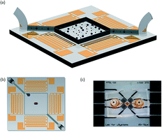
Acoustic fields offer a versatile and non-contact method for particle and cell manipulation, where several acoustofluidic systems have been developed for the purpose of sorting. However, in almost all cases, these systems utilize a steady flow to either define the exposure time to the acoustic field or to counteract the acoustic forces. Batch-based systems, within which sorting occurs in a confined volume, are compatible with smaller sample volumes without the need for externally pumped flow, though remain relatively underdeveloped. Here, the effects of utilizing a combination of travelling and standing waves on particles of different sizes are examined. We use a pressure field combining both travelling and standing wave components along with a swept excitation frequency, to collect and isolate particles of different sizes in a static fluid volume. This mechanism is employed to demonstrate size-based deterministic sorting of particles. Specifically, 5.1 μm and 7 μm particles are separated using a frequency range from 60 MHz to 90 MHz, and 5.1 μm particles are separated from 3.1 μm using an excitation sweeping between 70 MHz and 120 MHz.

---

Introduction

Particle and cell separation is a fundamental step in a number of biological and industrial processes, where many methodologies accomplish this separation in a continuous throughput manner. Many of these devices operate by combining fluid drag forces with an externally applied force including those arising from magnetic,^1,2 optical,^3,4 dielectrophoretic (DEP)^5–7 and acoustophoretic^8–11 fields, or using the flow profile of the fluid as it passes contractions or obstacles.^12,13 For each of these methods, particles with different dimensions, shapes, and electric or mechanical properties experience different forces and therefore displacements. The requirement for an externally generated continuous flow, however, limits the ability for these methods to be applied outside laboratory settings and usually necessitates external pumps with the minimum volume requirements that this entails.

In contrast, batch processing can be applied to small, μl-scale samples and increase diagnostic detection efficacy, crucial in many biological processes.^14–16 The ability to perform sample preparation on-chip reduces time investment; this compliments the reduction of reagent usage, allowing low operational costs. Despite these advantages, there have been comparatively few studies in particle separation for static fluids. Previous methodologies for the batch-sorting of small samples include optical tweezers,¹⁷ magnetic actuation¹ and locally induced flow from acoustic¹⁸ or electrohydrodynamic streaming.¹⁹ These methods are limited, however, in their separation efficiency (flow-based methods), complexity of operation (optical methods), or types of particles/cells that can be separated (magnetic methods). To tackle this, acoustic actuation offers easy on chip integration, the ability to use portable miniaturized circuits to actuate the acoustic field²⁰ and good biocompatibility.^21,22 In addition, acoustic force fields can be displaced²³ which permits the generation of particle mobility that is required for separation within a static fluid volume.

The disturbance of an acoustic field due to the presence of a particle, specifically one that differs in density and/or speed of sound with respect to the surrounding medium, results in a time-averaged acoustic radiation force (ARF) that acts on the particle. The force is a result of second order terms in the Navier–Stokes equation, which time-average over an oscillation to a non-zero value. As such the ARF acting on a particle leads to a net movement rather than an oscillation.²⁴ Whilst acoustic fields also lead to Bjerknes forces (forces arising from the scattered wave from a nearby particle) and acoustic streaming (a steady state swirling fluid motion), it is the acoustic radiation force which is most widely exploited for particle manipulation. Typically, this is through the excitation of either bulk acoustic waves^25–28 (BAW) or surface acoustic waves^29–31 (SAW). The former seeks to excite resonances within the fluid volume using longitudinal or flexural modes coupled from a vibrating structure; the latter uses a spatially periodic electrical field to create a resonant condition on a piezoelectric substrate. In the case of SAW, a further distinction can be made between travelling SAWs (TSAWs), in which a wave propagates through the system, and standing SAWs (SSAWs) in which there are two counter propagating waves. Sorting within a continuous flowing fluid has been achieved using BAW,^32–34 TSAW^31,35–39 and SSAW.^40,41 In batch systems, with very small samples in contact with a substrate, separation has been shown using acoustic streaming in droplets,¹⁸ in an open chamber⁴² and in a channel.⁴³

Here, we examine the use of acoustic radiation forces alone for particle separation in a batch system, and demonstrate that the controllability of this type of acoustic force allows highly specific separation. Our method utilizes a combination of several mechanisms made possible by SAW based actuation. Firstly and uniquely, we utilise both TSAW and SSAW; the former acts to push the particles across the chamber, the latter to capture particles in bands of minimum force potential. Secondly, we sweep the frequency of excitation, in doing so we average the force fields over a wide frequency range. Such an approach has been used to refine the force field in a droplet,⁴⁴ handle particles in multiple chambers,⁴⁵ and migrate particles across a chamber in a moving standing wave.⁴⁶ While the usage here is most akin to the latter example, we show that the final location of the particles is size dependant due to the addition of the travelling wave to the swept standing wave. Thirdly, utilising the ability of SAW systems to operate at high frequencies,⁴⁷ we are able to generate wavelengths, λ_f, that approach the diameter of the larger particles. Forces generated by TSAW and SSAW scale differently to particle radius, r (F_TSAW ∝ r⁶,³⁵ and F_SSAW ∝ r³,²⁴ if particle radius, r ≪ λ_f). Furthermore, Skowronek et al.⁴⁸ demonstrated that TSAW is effective for particle deflection when the parameter, κ ≥ 1.28 ± 0.20, where κ = k × r (k is the wavenumber in the fluid). Hence the relative importance of each force type is particle size dependant; we show that the difference in response this gives rise to is further enhanced as λ_f approaches the size of the larger particle, r_large to operate above the critical κ parameter.⁴⁹

We show that the cut-off radius between behaviour types (TSAW or SSAW dominated) is frequency range dependant, and demonstrate the separation of 3.1 μm from 5.1 μm particles, as well as 5.1 μm from 7 μm within a static sample.

Operating principle

Experimental

The system consists of a microfluidic chamber, cast in polydimethylsiloxane (PDMS), and bonded onto a 128° rotated Y-cut X-propagating lithium niobate, LiNbO₃ (LN) piezoelectric substrate. This substrate is patterned with four sets (each aligned 45° from the X-axis) of aluminium interdigital transducers (IDTs), which are arranged in two pairs arranged orthogonally to each other (Fig. 1). The speed of sound in LN differs with respect to the propagation direction, here in this setup it is approximately 3600 m s⁻¹.⁵⁰ Each set of IDTs is chirped,⁵¹ meaning that there is a spatial variation in pitch between the electrodes (SAW wavelength, λ_SAW range; 20–70 μm), making them responsive to a range of frequencies. Each set of transducers consists of 34 finger pairs with individual finger widths between 20 μm and 70 μm with an aperture of 1140 μm. The actuation of two pairs of orthogonally oriented sets of IDTs permits the generation of a 2D acoustic field⁵² within the microfluidic chamber when an oscillating (i.e. A/C) electrical signal is applied. This field can have both standing and travelling wave components, whose relative magnitudes depend on the power applied to each set of IDTs.

Fig. 1 (a) Diagram of the batch sorting device used in the experimental setup (particles dispersed homogenously as an initial condition) the chamber size is 707 μm (W) × 707 μm (L) × 25 μm (H), (b) top view of the idealised particle batch sorting (smaller particles (red) congregate in the centre and the larger particles (blue) at the top left corner) and (c) picture of the device used.

The device is held under a microscope (Olympus BX43) using a 3D printed frame where spring loaded contact pins make contact with the electrode pads on the LN substrate. The experiments are recoded at 15 frames per second using a microscope mounted camera (Dino-Eye AM4023CT). The electrical signal is provided by a combined signal generator and amplifier (Rohde &Schwarz HAMEG HM8134-3 and Amplifier Research 25A250A). This generator is capable of providing a swept frequency signal, in which the frequency is constantly changed from a lower frequency limit, f_L, to a higher frequency limit, f_H, in 1 MHz steps, with a set cycle time period, T_CYCLE. For separation of 3.1 and 5.1 μm particles a 70–120 MHz signal range over with T_CYCLE = 10.3 s was used. For separating 5.1 μm and 7 μm the frequency range and T_CYCLE are 60–90 MHz and 6.45 s, respectively. The S₁₁ values, a measure of input port voltage reflection coefficient (i.e. efficiency of the examined IDT; power transmitted into the LN to generate SAW) were assayed using a network analyser (PowerSAW Belektronig F20).

Analysis of the fluorescent particles intensity in the captured images allows time dependant data to be gathered on the collection of the particles. Firstly, a suitable RGB threshold was applied to the entire image such that areas in which a particle was present were attributed the value of 1 and the remaining areas the value of 0. Two areas measuring 100 × 100 pixels in the locations where the particles finish were identified, and the intensity analysed. The location of these areas was held constant throughout comparable experiments. The average intensity was then calculated for 5 distinct equally spaced time steps. To allow for a comparison over different samples accommodating for varying initial particle counts and distributions, the average intensity of each particle size is normalised by the total average intensity of both particle sizes within the analysis regions at corresponding time steps. It is this normalised average intensity distribution within the two regions which are used to demonstrate particle separation.

Numerical simulation

The forces exerted on a particle that is much smaller than the acoustic wavelength are well understood for both standing waves²⁴ (SWs) and travelling waves⁵³ (TWs), though the simultaneous effects of both these wave components has not been investigated. In this work, a combination of these two types of waves and the effect it has on particles of various sizes are presented. The acoustic radiation force is a non-linear effect, arising from second order terms. This means that whilst the pressure fields arising from each of the wave types can be summed, such linear superposition is not possible for the force fields acting upon particle sizes that a comparable to the wavelength as investigated here.⁵⁴ To illustrate the effect of a mixed wave field in what is a complex system, a simple 2D model capturing the salient features has been developed using COMSOL Multiphysics. This model incorporates the effects of the TSAW and SSAW forces, though use of a swept frequency will not be examined.

When an acoustic wave encounters a suspended object (with differing density and/or speed of sound to the suspending medium) the wave will be diffracted and scattered. In order to avoid reflections such as those arising from a scattered wave, the fluid volume has been made long and thin, see Fig. 2(a). The upper and lower boundaries are such that a matched acoustic impedance boundary condition is imposed; this means that any scattered wave will propagate through it and reflections will be avoided. At each end of the chamber, boundary conditions need to be established such that a range of combinations of standing and travelling wave can be investigated. This necessitates a different boundary condition, so to keep scattered wave reflection to a minimum, these boundaries are located a long way from the scattering object and the boundaries are kept short. Each end of the chamber acts as a wave source; by keeping the edges narrow the fields that emerge in the centre of the chamber are in the far field region of the ultrasonic source^55,56 and so represent a reasonable approximation of a uniform sinusoidal waveform.

Fig. 2 (a) FE model depicting boundary conditions and 2nd order time averaged absolute pressure distribution when (i) R = 0.5 (mixed SW/TW), (ii) R = 0 (pure TW) and (iii) R = 1 (pure SW), (b) plot of the 2nd order time-averaged pressure field against the X-position (1 λ_f shown) for different R values.

The amplitude of the leftward propagating wave is set to be a ratio (<1), R, of the rightward wave. This imbalance leads to a pressure field consisting of a standing wave (amplitude proportional to R, the standing wave ratio) and travelling wave (amplitude proportional to 1 − R) component in the centre of the chamber, labelled the area of interest in Fig. 2(a) (14λ_f from each end). Each end of the chamber also has a matched acoustic boundary layer, which allows waves of a defined wavenumber to pass through without reflection.

This model investigates the effects of the particle within a pressure field of a certain wavelength and does not directly simulate the piezoelectric LN substrate as we are primarily interested in the interaction between a particle and a combined SW/TW pressure field. The particle is assigned the same material properties as the polystyrene fluorescent particles used in the experiments (ρ_p = 1050 kg m⁻³, c_p = 2350 m s⁻¹).

The time-averaged force acting on a solid particle of arbitrary size when the fluid viscosity is neglected can be calculated using:⁵⁷

where, ρ_f and c_f (1000 kg m⁻³ and 1490 m s⁻¹) are the density and speed of sound of the fluid respectively, and v₁² and p₁² are the mean square fluctuation of the velocity and pressure respectively. The forces calculated have been benchmarked against cases shown by Dual et al.⁵⁷ In the pressure fields considered, the SSAW and TSAW forces on a particle are assessed over a distance of λ_f (from −λ_f/2 to λ_f/2 at λ_f/12 intervals).

Results and discussions

Numerical results

When a particle is located within the pressure field (Fig. 3(a)), eqn (1) can be used to calculate the forces acting on its surface over a single oscillation cycle, examples are shown in Fig. 3(b) to (d). The acoustic contrast between the particle and the fluid medium gives rise to these forces while also distorting the local pressure field. Fig. 3(e) shows the total force (i.e. after integration over the particle surface) as a function of radius, r, for both pure travelling wave and a pure standing wave. This allows a link to be made with established theories, in which the scaling with radius is known to differ; for a sphere, F_TSAW ∝ r⁶,³⁵ and F_SSAW ∝ r³,²⁴ provided r ≪ λ_f. This difference in the relationship means that a larger particle is subject to a larger TSAW induced force than is a smaller one. What this figure shows is that as the radius is increased so that r approaches λ_f, this difference is further enhanced as the increase in force associated with the SW tapers off at a certain r value as it is increased, whereas F_TSAW continues to increase, yielding an r_crit above which F_TSAW > F_SSAW. Hence, to increase the influence of the travelling wave and so the sorting effect, smaller wavelengths should be used, thus increasing the size of the particle relative to the wavelength.

Fig. 3 2nd order time averaged absolute pressure distribution when R = 0.3 (i.e. 30% standing wave) (λ_f = 30 μm; P = 1 MPa) with (a) a 1 μm particle placed at from the centre, an acoustic radiation force (ARF) arrow plot (normalised arrows visualise the relative magnitude of the ARF acting at it's corresponding location)with particle sizes (b) 3 μm, (c) 5 μm and (d) 10 μm placed in the same location as (a) (colour bar scale units in Pa), (e) force, F by the 2nd order time averaged absolute pressure, <P> plotted against particle radius, r in μm for a pure TSAW (blue) and a pure SSAW (red).

Both the orientation of the forces and the influence of the particle on the force field can be seen for increasing particle sizes in Fig. 3(b)–(d). In each case the particle is located in the same location, leftward of the pressure antinode, so a pure standing wave would act to move the particle further leftward towards the pressure node. Conversely, a pure TW acts to push the particle in the wave's propagation direction, hence rightward. It can be seen, from Fig. 3(b)–(d) the net force on the smallest, 3 μm, particles is leftward (toward the nodal position), whilst for the 5 μm and 10 μm particles is rightward, hence the change between dominance of SW and TW is shown as radius dependant (R value held constant at 0.3).

Fig. 3 addresses the dominant force at one location. In order to map out the spatial force field the simulated particle is sequentially translated with reference to the field, the resulting net force variation is shown in Fig. 4(a) and (b) for two different R values (1, 0.2) and three particle sizes (1, 4, and 7 μm). What can be seen is that for certain combinations of these two parameters the force is never negative, hence always rightward in nature, i.e. the TW force dominates over the whole wavelength. If the non-dimensional size of a particle, a = r/λ_f, is above a critical size, a_crit = r_crit/λ_f, the particle's trajectory (at all locations of a wavelength) will be dictated by the TW and migrate rightward, otherwise if a < a_crit the particle will ultimately be held in one location (where F = 0 and dF/dx is negative). As expected in the pure SW scenario, Fig. 4(a), all three particle sizes will migrate to fixed locations. However, for an R value of 0.2, Fig. 4(b), the 7 μm will migrate rightward, whilst the 1 μm and 4 μm particles will be held static. This model demonstrates the principle of size based separation by use of a TW and SW, whereby larger particles are preferentially translated in this hybrid field.

Fig. 4 FE model calculated ARF in the X-direction against X-position from the centre of the chamber (λ_f = 30 μm) with (a) R = 1 (i.e. 100% SSAW) and (b) R = 0.2 (i.e. 20% SSAW). (c) Minimum calculated ARF at against R for various particle sizes in μm, and (d) crossover SW ratio (i.e. ratio at which the SW becomes more dominant than the TW) against particle radius, r.

Fig. 4(c) shows the value of the minimum force over a wavelength as a function of the standing wave ratio, R for a range of particle sizes. The plot shows that as the value of R increases, the dominant component of the acoustic field transitions from TSAW to SSAW gradually and thus the potential to tune r_crit. This is further demonstrated by plotting the value of a_c against R, Fig. 4(d) shows the crossover R value for a given r. Bearing in mind that the value of R is a measure of the relative amplitude, and so dominance, of the TW and SW, Fig. 3(e) also indicates, indirectly, a mechanism to tune the critical particle system, by operating at a lower or higher frequency the relative strength of the force generated due to TW or SW is altered, and hence the relative importance of these two wave components can be altered by R or frequency change (i.e. change in λ_f).

Experimental results

The numerical results demonstrate several aspects of the underlying physics allowing particle separation, however it does not address the effect of sweeping the frequency of excitation. This plays two key roles; firstly, when considering the balance between the SW and TW it enhances the TW effect, and secondly when considering particle dominated by the SW, it causes collection into a single location rather than large number of static pressure nodes due to the time-averaged effect of the force field.⁴⁶

The R value, determining the balance between TW and SW, of the experimental system is set by the differing response of the IDTs to the electrical signal. The effective actuation amplitude is dependent on the S₁₁ of the IDTs. The S₁₁ parameter is the reflection coefficient due to the electrical impedance mismatch between the IDTs and the power source (this includes the influence of cables and electrical connectors). The S₁₁ curves of the IDTs based on an identical electrical input signal are shown in Fig. 5(a), it can be seen that despite nominally identical electrode patterns, there are differences in these plots. By sweeping the frequency over a range, inevitably some part of this bandwidth will display differing S₁₁. Within this subset of frequencies, there will be a TW component as well as a SW component. The amplitude of the wave produced by each IDT set depends on the S₁₁ parameter of the corresponding IDT. For instance, if an IDT set has a S₁₁ parameter of 0.6, the transmitted electrical signal amplitude to that particular IDT is 40% (i.e. (1 − S₁₁) × 100%) of the input power. Therefore, the lower the S₁₁ parameter, more electrical power is transmitted to the IDT set. Here, the amplitudes (for an identical input electrical signal) of the SW and TW respectively, at a given frequency, are A₁ and A₂ − A₁, where A₁ and A₂ are the wave amplitudes of the weaker and stronger sources respectively, for frequencies below 105 MHz. A larger S₁₁ at a given frequency, as indicated in Fig. 5(a), means a weaker SAW (i.e. lower wave amplitude) emanating from that IDT (i.e. IDT 1 in this scenario). The effect of the variations in S₁₁ is demonstrated in Fig. 5(b) which shows the spatial variation of surface displacement, measured by Laser Doppler Vibrometer (Polytec UHF-120) occurring between the IDTs when all four are actuated by the same electrical input. If the peak (marked by the black square in Fig. 5(b)) displacement magnitude is observed, the peak in Fig. 5(b)(i and iii) are similar, however, Fig. 5(b)(ii) has a smaller magnitude (i.e. lighter red comparatively; colour bar scale is identical for all three images). This is due to the presence of a TW and SW combination whereby, the resultant magnitude of a wave differs throughout a complete oscillation as depicted by the normalised amplitude plot in Fig. 5(b)(iv) corresponding to the same phase presented. The presence of different displacement magnitude peaks as shown in Fig. 5(b) would not be observed in a pure SW or TW system but only with a combination of SW and TW.

Fig. 5 (a) S₁₁ parameter curve against frequency, f for each of the IDTs used as denoted by the inset (i) (arrow lengths depict the relative power transmitted to the corresponding IDT at 95 MHz). The value of 1 − S₁₁ parameter, denotes the power transmitted to the device leading to the power disparity within the system giving rise to a combination of TSAW and SSAW. (b) Time series images of Laser Doppler Vibrometer (LDV) scan data demonstrating the presence of the TSAW at 95 MHz every rad phase (black line denotes centre diagonal of the scan area (constant position); black square denotes the tracked wave peak) (i) 0 rad (ii) rad (iii) π rad and (iv) depiction of normalised magnitude, A when R = 0.3 against X position at 3 different time intervals within a period (increments of rad) (1 λ_SAW shown).

As observed in Fig. 5(a) the differences in S_11, thus, differences in the amplitudes of the waves are relatively small, less than the values of R used in the simulations. The reason is due to the frequency sweep. For a pure standing wave, the particles will move from the force potential minima, U (not to be confused with force, F; where F = −∇U) at one frequency, to that of the next frequency, this will bring them closer to the centre of the chamber, with each frequency change, as each minima is offset from the previous one. In the context of single frequency of operation, as in Fig. 4, for TW dominated behaviour there are no local force potential minima. However, if the frequency is swept this condition is relaxed.

For the sake of simplicity in describing the phenomenon, we consider a simplified 1-dimensional system (it should be noted that the system utilised here in experiments is a 2-dimensional system), where a leftward TW component is added to the SW force potential (i.e. a slope is added to a sine wave). When the distance between the rightward local maxima and the local minima (d_a) is larger than between the same local minima and the local leftward maxima (d_b), we term this an asymmetrical force potential. To bring particles to the centre (in the 1-dimensional case) from the right-hand side is straightforward; it follows the pure SW case, but with further assistance from the TW. What is more interesting is the behaviour on the left-hand side of the chamber as this is where the two particle sizes behave differently. The minima of the SW dominated particles may be offset such that the particles are drawn to the centre (the offset is <1/2(d_a + d_b)), however due to the force potential asymmetry the same stepwise changing of the frequency could lead to a particle jumping from one local minima to the next leftward one if the offset exceeds d_b. Hence, even if local minima are present in the force potential, the use of a swept frequency system can mean that the TW causes migration away from the larger source (i.e. A₂ & A₄ for the case shown in Fig. 5(b)). Indeed, when a single frequency (120 MHz) was used, no difference in behaviour was observed between 3.1 μm and 5.1 μm diameter particles, i.e. neither were TW dominated. The power transmitted to each set of IDTs was not actively altered. As shown by Fig. 5(a), a disparity is observed for the IDT design used and therefore active control was not required to demonstrate the sorting mechanism. However, if precise control of the TW dominated particle's final location is required, active control of input power to individual sets of IDTs can be implemented.

The role of sweeping the frequency for SW dominated particles is to cause a longer migration trajectory than simply between an antinode and the nearest node in a single frequency system. Fig. 6 shows how, 5.1 μm particles (dominated by SW effects, with a < a_crit) are first trapped in distinct locations at the pressure nodes⁵⁴ of a 2-dimensional field at a single frequency, and then as the frequency is raised from 60 MHz to 90 MHz, and the cycle repeated, gradually migrate to the centre of the chamber as result of the averaged force field over a sweep cycle.

Fig. 6 (a) The orientation of the chamber in relation to the IDTs and depiction of the relative transmitter power for 90 MHz (i.e. f_H). Time series of images (depicted square is the entire chamber as shown in Fig. 1(a) as seen from above) demonstrating 5 μm particle collection dominated by SSAW as a result of the sweep over a range (60–90 MHz (1 MHz interval); 400 mV) of frequencies (T₅ = 45 s; 7 sweep cycles). From the initial dispersion (b) to the final position (f) (scale is equal over all images). See ESI Video 1† for multimedia.

Whilst particles dominated by the SW will migrate to the centre of the chamber when the frequency is swept, those dominated by the TW (over some part of the frequency sweep) will migrate away from the larger amplitude source (or sources if 4 IDTs are used). To demonstrate this, the microfluidic chamber was filled with fluorescent polystyrene particles of 2 distinct sizes and the IDTs actuated. In the first case, a sample with 5.1 μm (green) and 7 μm (yellow) particles were separated using a frequency range of 60 MHz (f_L) to 90 MHz (f_H) with a T_CYCLE of 6.45 s. As shown in Fig. 7(a), the particles are initially dispersed throughout the chamber. Once the IDTs are excited, particles of both sizes are translated, with smaller particles shifted to the chamber centre. Midway through the experiment (T₃) most of the smaller 5.1 μm particles have been concentrated at the middle of the chamber as a result of the dominant SSAW (a_{5 μm} < a_crit). In contrast, the 7 μm particles (a_{7 μm} > a_crit) migrate to the top left corner of the chamber (i.e. A₂ & A₄ > A₁ & A₃; see relative power depiction in Fig. 7(a)). The bar graphs in Fig. 7(b)(i and ii) show the percentage of each particle within two areas of the chamber (see Fig. 7(a) for their location) as a function of normalized intensity. It can be seen that over time the proportion of 5.1 μm particles increase to 100% and the proportion of 7 μm particles decrease consistently at the centre of the chamber. In contrast, in Fig. 7(b)(ii), it can be observed that, the proportion of larger 7 μm particles increases while the smaller 5.1 μm particles decrease. It should be noted that the appearance of the yellow 7 μm particle present in the middle of the chamber as seen in Fig. 7(a) T₄ is due to particle migration drifting from the chamber outlet. However, this particle is also forced towards to the larger particle collection region (see ESI Video 2†). The total time to achieve complete separation of 5.1 μm and 7 μm particles excited at 350 mV is 115 s. The data presented is the average over 3 trials; the error bars show one standard deviation. As the initial location of the particles is random and the final position is determined by the response the acoustic field, it is clear that the error bars reduce significantly as the experiment progresses.

Fig. 7 (a) Chamber orientation and relative transmitted power depiction (at 90 MHz (i.e. f_H)) along with time sequence images of experimental data for particle separation of 5 μm (green) and 7 μm (yellow) particles (depicted square is the entire chamber as shown in Fig. 1(a) as seen from above) (scale is equal over all images) (see ESI video 2† for multimedia) and (b) average intensity percentage against time analysis data (i) centre of chamber (i.e. as depicted by the green square in (a)) (ii) side of chamber (i.e. as depicted by the red square in (a)) (350 mV; T₅ = 115 s). (c) Average intensity percentage against time analysis data based on experimental data of particle separation for 3.1 μm and 5.1 μm particles (i) centre of chamber (i.e. as depicted by the green square in (a)) (ii) side of chamber (i.e. as depicted by the red square in (a)) (250 mV; T₅ = 210 s).

In Fig. 7(c), samples of 3.1 μm and 5.1 μm particles have been successfully separated. Again linking back to Fig. 4(b), to enter the regime in which TW becomes increasingly important the particle size needs to approach the wavelength, as the particles being separated are smaller in this experiment, this means an increase in frequency is required. Consequently, the excitation frequency range is increased, and set at 70 MHz (f_L) to 120 MHz (f_H) over a time period of 10.3 s. It can be seen that under these operational conditions the 3.1 μm particles collect at the center of the chamber whilst the 5.1 μm particles migrate away from IDTs 1 & 3 (i.e. stronger sources; see S₁₁ curve in Fig. 5(a) at 120 MHz). In this case, the larger 5.1 μm particles migrate to the bottom right corner where, A₁ & A₃ > A₂ & A₄ as opposed to the earlier case whereby, A₂ & A₄ > A₁ & A₃. As such, the use of frequency range to tune the critical particle size for separation is demonstrated. The total time to achieve complete separation of 3.1 μm and 5.1 μm particles excited at 250 mV is 210 s.

Conclusions

The concentration and size-based separation of particles has been demonstrated in a static flow condition by exploiting a pressure field that combines both standing and travelling waves. These are excited by generation of counter propagating surface acoustic waves and modified using a continuously swept excitation frequency. Separation occurs due to the hitherto unexplored interplay between travelling and standing wave forces as the particle size approaches the acoustic wavelength, where the travelling wave force can exceed that of the standing wave. The use of a swept frequency further accentuates the effect of the travelling wave on larger particles and causes smaller particle migration with the moving standing wave field resulting in concentration from the entire volume of the sample chamber (rather than a quarter wavelength as for a single frequency excitation). The result is the larger particles are pushed across the chamber dominated by the travelling wave component, and smaller particles are collected at the center of the chamber due to the standing wave component. We demonstrate this methodology in the deterministic separation of 5.1 μm and 7 μm particles using a frequency range from 60 MHz to 90 MHz, and 5.1 μm from 3.1 μm particles using an excitation frequency range of 70 MHz to 120 MHz.

Acknowledgements

We gratefully acknowledge support received from the Australian Research Council, Grant No. DP110104010. This work was performed in part at the Melbourne Centre for Nanofabrication (MCN) in the Victorian Node of the Australian National Fabrication Facility (ANFF).

References

1. Y. Wang, Y. Zhao and S. K. Cho, J. Micromech. Microeng., 2007, 17, 2148.
2. N. Xia, T. Hunt, B. Mayers, E. Alsberg, G. Whitesides, R. Westervelt and D. Ingber, Biomed. Microdevices, 2006, 8, 299–308.
3. M. P. MacDonald, G. C. Spalding and K. Dholakia, Nature, 2003, 426, 421–424.
4. B. Landenberger, H. Höfemann, S. Wadle and A. Rohrbach, Lab Chip, 2012, 12, 3177–3183.
5. H. Shafiee, M. B. Sano, E. A. Henslee, J. L. Caldwell and R. V. Davalos, Lab Chip, 2010, 10, 438–445.
6. P. R. C. Gascoyne and J. Vykoukal, Electrophoresis, 2002, 23, 1973–1983.
7. S. Park, Y. Zhang, T.-H. Wang and S. Yang, Lab Chip, 2011, 11, 2893–2900.
8. J. Nam, Y. Lee and S. Shin, Microfluid. Nanofluid., 2011, 11, 317–326.
9. J. Nam, H. Lim, D. Kim and S. Shin, Lab Chip, 2011, 11, 3361–3364.
10. J. Shi, H. Huang, Z. Stratton, Y. Huang and T. J. Huang, Lab Chip, 2009, 9, 3354–3359.
11. F. Petersson, A. Nilsson, C. Holm, H. Jönsson and T. Laurell, Lab Chip, 2005, 5, 20–22.
12. M. Yamada, M. Nakashima and M. Seki, Anal. Chem., 2004, 76, 5465–5471.
13. J. McGrath, M. Jimenez and H. Bridle, Lab Chip, 2014, 14, 4139–4158.
14. H. M. Davey and D. B. Kell, Microbiol. Rev., 1996, 60, 641–696.
15. N. Sivanantha, C. Ma, D. J. Collins, M. Sesen, J. Brenker, R. L. Coppel, A. Neild and T. Alan, Appl. Phys. Lett., 2014, 105, 103704.
16. M. Eisenstein, Nature, 2006, 441, 1179–1185.
17. Y. Tan, D. Sun, J. Wang and W. Huang, IEEE Trans. Biomed. Eng., 2010, 57, 1816–1825.
18. P. R. Rogers, J. R. Friend and L. Y. Yeo, Lab Chip, 2010, 10, 2979–2985.
19. L. Y. Yeo, D. Lastochkin, S.-C. Wang and H.-C. Chang, Phys. Rev. Lett., 2004, 92, 133902.
20. L. Y. Yeo and J. R. Friend, Biomicrofluidics, 2009, 3, 012002.
21. J. Hultström, O. Manneberg, K. Dopf, H. M. Hertz, H. Brismar and M. Wiklund, Ultrasound in Medicine and Biology, 2007, 33, 145–151.
22. D. Bazou, R. Kearney, F. Mansergh, C. Bourdon, J. Farrar and M. Wride, Ultrasound in Medicine and Biology, 2011, 37, 321–330.
23. X. Ding, S.-C. S. Lin, B. Kiraly, H. Yue, S. Li, I.-K. Chiang, J. Shi, S. J. Benkovic and T. J. Huang, Proc. Natl. Acad. Sci. U. S. A., 2012, 109, 11105–11109.
24. L. P. Gor'Kov, Sov. Phys. Dokl., 1962, 6, 773–775.
25. M. Hill, R. J. Townsend and N. R. Harris, Ultrasonics, 2008, 48, 521–528.
26. P. Glynne-Jones, C. E. M. Demore, Y. Congwei, Q. Yongqiang, S. Cochran and M. Hill, IEEE Trans. Ultrason. Ferroelectrics Freq. Contr., 2012, 59, 1258–1266.
27. A. Neild, S. Oberti and J. Dual, Sens. Actuators, B, 2007, 121, 452–461.
28. I. Leibacher, S. Schatzer and J. Dual, Lab Chip, 2014, 14, 463–470.
29. M. Sesen, T. Alan and A. Neild, Lab Chip, 2014, 14, 3325–3333.
30. D. J. Collins, T. Alan, K. Helmerson and A. Neild, Lab Chip, 2013, 13, 3225–3231.
31. D. J. Collins, A. Neild and Y. Ai, Lab Chip, 2016 10.1039/c5lc01335f.
32. L. Johansson, F. Nikolajeff, S. Johansson and S. Thorslund, Anal. Chem., 2009, 81, 5188–5196.
33. T. Laurell, F. Petersson and A. Nilsson, Chem. Soc. Rev., 2007, 36, 492–506.
34. A. Lenshof and T. Laurell, Chem. Soc. Rev., 2010, 39, 1203–1217.
35. G. Destgeer, K. H. Lee, J. H. Jung, A. Alazzam and H. J. Sung, Lab Chip, 2013, 13, 4210–4216.
36. T. Franke, S. Braunmuller, L. Schmid, A. Wixforth and D. A. Weitz, Lab Chip, 2010, 10, 789–794.
37. L. Schmid, D. A. Weitz and T. Franke, Lab Chip, 2014, 14, 3710–3718.
38. G. Destgeer, B. H. Ha, J. H. Jung and H. J. Sung, Lab Chip, 2014, 14, 4665–4672.
39. G. Destgeer, B. H. Ha, J. Park, J. H. Jung, A. Alazzam and H. J. Sung, Anal. Chem., 2015, 87, 4627–4632.
40. X. Ding, S.-C. S. Lin, M. I. Lapsley, S. Li, X. Guo, C. Y. Chan, I.-K. Chiang, L. Wang, J. P. McCoy and T. J. Huang, Lab Chip, 2012, 12, 4228–4231.
41. D. J. Collins, T. Alan and A. Neild, Lab Chip, 2014, 14, 1595–1603.
42. P. Rogers, I. Gralinski, C. Galtry and A. Neild, Microfluid. Nanofluid., 2013, 14, 469–477.
43. C. Devendran, I. Gralinski and A. Neild, Microfluid. Nanofluid., 2014, 17, 879–890.
44. S. Oberti, A. Neild, R. Quach and J. Dual, Ultrasonics, 2009, 49, 47–52.
45. B. Vanherberghen, O. Manneberg, A. Christakou, T. Frisk, M. Ohlin, H. M. Hertz, B. Onfelt and M. Wiklund, Lab Chip, 2010, 10, 2727–2732.
46. A. Haake, A. Neild, G. Radziwill and J. Dual, Biotechnol. Bioeng., 2005, 92, 8–14.
47. R. J. Shilton, M. Travagliati, F. Beltram and M. Cecchini, Adv. Mater., 2014, 26, 4941–4946.
48. V. Skowronek, R. W. Rambach, L. Schmid, K. Haase and T. Franke, Analytical chemistry, 2013, 85, 9955–9959.
49. G. Destgeer and H. J. Sung, Lab Chip, 2015, 15, 2722–2738.
50. A. Holm, Q. Stürzer, Y. Xu and R. Weigel, Microelectron. Eng., 1996, 31, 123–127.
51. V. M. Ristic, Principles of acoustic devices, Wiley, New York, 1983.
52. D. J. Collins, B. Morahan, J. Garcia-Bustos, C. Doerig, M. Plebanski and A. Neild, Nat. Commun., 2015, 6, 8686.
53. K. Yosioka and Y. Kawasima, Acustica, 1955, 5, 167–173.
54. S. Oberti, A. Neild and J. Dual, J. Acoust. Soc. Am., 2007, 121, 778.
55. A. Holm, P. Wallner, W. Ruile and R. Weigel, Ultrason. Symp. Proc., 1997, 1, 153–156.
56. A. Neild, D. Hutchins, T. Robertson, L. Davis and D. Billson, Ultrasonics, 2005, 43, 183–195.
57. J. Dual, P. Hahn, I. Leibacher, D. Moller, T. Schwarz and J. Wang, Lab Chip, 2012, 12, 4010–4021.

---

Footnote

† Electronic supplementary information (ESI) available. See DOI: 10.1039/c5ra26965b

---