DOI:
10.1039/C5SM01412C
(Paper)
Soft Matter, 2015,
11, 6680-6691
Virial pressure in systems of spherical active Brownian particles
Received
8th June 2015
, Accepted 14th July 2015
First published on 16th July 2015
Abstract
The pressure of suspensions of self-propelled objects is studied theoretically and by simulation of spherical active Brownian particles (ABPs). We show that for certain geometries, the mechanical pressure as force/area of confined systems can be equally expressed by bulk properties, which implies the existence of a nonequilibrium equation of state. Exploiting the virial theorem, we derive expressions for the pressure of ABPs confined by solid walls or exposed to periodic boundary conditions. In both cases, the pressure comprises three contributions: the ideal-gas pressure due to white-noise random forces, an activity-induced pressure (“swim pressure”), which can be expressed in terms of a product of the bare and a mean effective particle velocity, and the contribution by interparticle forces. We find that the pressure of spherical ABPs in confined systems explicitly depends on the presence of the confining walls and the particle–wall interactions, which has no correspondence in systems with periodic boundary conditions. Our simulations of three-dimensional ABPs in systems with periodic boundary conditions reveal a pressure–concentration dependence that becomes increasingly nonmonotonic with increasing activity. Above a critical activity and ABP concentration, a phase transition occurs, which is reflected in a rapid and steep change of the pressure. We present and discuss the pressure for various activities and analyse the contributions of the individual pressure components.
1 Introduction
Living matter composed of active particles, which convert internal energy into systematic translational motion, is a particular class of materials typically far from equilibrium. Examples range from the microscopic scale of bacterial suspensions1 to the macroscopic scale of flocks of birds and mammalian herds.2 Such active systems exhibit remarkable nonequilibrium phenomena and emergent behavior like swarming,3–7 turbulence,6 activity-induced clustering and phase transitions,8–21 and a shift of the glass-transition temperature.21,22 The nonequilibrium character of active matter poses particular challenges for a theoretical description. In particular, a thermodynamic description is missing, but would be desirable in order to be able to define elementary thermodynamic variables such as temperature or chemical potential.23 Considerable progress in the description of activity-induced phase transitions has been achieved recently.14,23–30
Pressure in active fluids has attracted considerable attention lately, because mechanical pressure as force per area can be defined far from equilibrium and might be useful to derive a nonequilibrium equation of state.13,23,31–33 Interestingly, simulation studies reveal such an equation of state, with a van der Waals-type pressure–volume phase diagram typical for gas–liquid coexistence.13,23,31,32
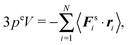
In thermal equilibrium, pressure can be equivalently defined in various ways. In addition to the mechanical definition, pressure p follows as a derivative with respect to volume V of the Helmholtz free energy F, i.e., p = −(∂F/∂V)T,N, at constant temperature T and particle number N.34 Moreover, the virial theorem can be exploited.34–37 These two identical formulations relate the surface pressure to bulk properties. However, for nonequilibrium systems, it is a priori not evident how to relate surface pressure to bulk properties, as it has to be kept in mind that there is usually no free-energy functional. By now, pressure in active fluids has been calculated using various virial-type expressions,13,23,31 typically without a fundamental derivation. Basic relations are provided for two-dimensional fluids in ref. 23, starting from the mechanical definition of pressure and by exploiting the Fokker–Planck equation for the phase-space probability distribution.
Here, we apply the virial theorem to derive expressions for the pressure in active fluids. Both, fluids confined between solid walls and exposed to periodic boundary conditions are considered. As an important first step, we demonstrate that the mechanical pressure of a confined fluid can be equivalently represented by the virial of the surface forces for particular geometries such as a cuboid and a sphere. This has important implications, since it provides a relation of the mechanical pressure with bulk properties of the fluid.23 Based on this expression, we derive an internal expression for the pressure, which comprises the ideal gas pressure, a swim pressure due to particle propulsion, and a contribution by interparticle interactions. As a result, we find that the swim pressure of the spherical ABPs explicitly depends on the confining walls and the particle–wall interaction, in contrast to results presented in ref. 23, but in agreement with more general considerations of anisotropic bodies.27,38 Systems with periodic boundary conditions naturally lack such a term. Hence, walls can induce features in confined active systems, which will not appear in periodic systems.
By Brownian dynamics simulations, we determine pressure–concentration relationships of active Brownian particles in three-dimensional periodic systems for various propulsion velocities. As previously observed,13,23,31,39 we find an increasingly nonmonotonic behavior of the pressure with increasing propulsion velocity. Above a certain velocity, we also find a van der Waals-loop-type relation. Most importantly, however, we find an abrupt change of the pressure for phase-separating fluids. Thereby, the magnitude of the pressure jump increases with increasing propulsion velocity. Hence, we argue that the nonmonotonic behavior indicates increased density fluctuations of the active fluid, but a phase transition is reflected in a more pronounced abrupt change of the pressure. A detailed analysis of the individual contributions to the pressure shows that the main effect is due to the activity of the colloidal particles, which gives rise to a so-called swim pressure as introduced in ref. 31. However, also the interparticle-force contribution exhibits an abrupt increase above the phase-transition concentrations.
The paper is organized as follows. In Section 2, the model of the active fluid is presented. The dynamics of ABPs in a dilute system is analysed in Section 3 for confined and unconfined particles. Expressions for the virial pressure are derived in Section 4 for confined and periodic systems. Simulation results for periodic systems are presented in Section 5, and our findings are summarized in Section 6. Details of the stochastic dynamics of the ABPs are discussed in Appendices A and B. A derivation of the equilibrium pressure via the virial theorem is presented in Appendix C. Appendix D establishes the relation between the mechanical pressure and the surface virial for active systems.
2 Model
We consider a system of N active objects, which are represented by hard-sphere-like particles of diameter σ. A particle i is propelled with constant velocity v0 along its orientation vector ei in three dimensions (3D).8,16,17,21,40 Its translational motion is described by the Langevin equation| | 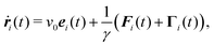 | (1) |
where ri is the particle position, ṙi the velocity, Fi the total force on the particle, γ the translational friction coefficient, and Γi a Gaussian white-noise random force, with the moments| | | 〈Γα,i(t)Γβ,j(t′)〉 = 2γkBTδαβδijδ(t − t′). | (3) |
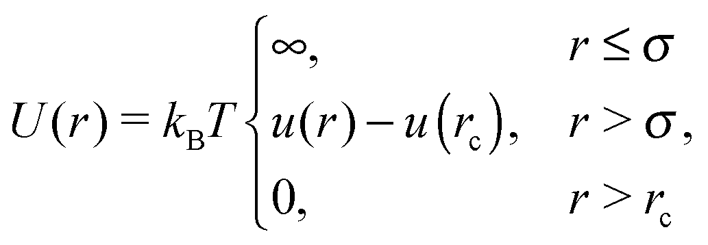
Here, T denotes the temperature in equilibrium, kB the Boltzmann constant, and α, β ∈ {x,y,x}. The friction coefficient γ is related to the translational diffusion coefficient D0tvia D0t = kBT/γ. The interparticle force is described by the repulsive (shifted) Yukawa-like potential| |  | (4) |
where u(r) = 5le−(r−σ)/l/(r − σ). Here, l is the interaction range and rc is the upper cut-off radius. The orientation ei performs a random walk according to| | | ėi(t) = ei(t) × ηi(t), | (5) |
where ηi(t) is a Gaussian white-noise random vector, with the moments| | | 〈ηα,i(t)ηβ,j(t′)〉 = 2Drδαβδijδ(t − t′). | (7) |
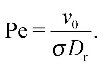
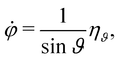
Eqn (5) is a stochastic equation with multiplicative noise. An equivalent representation for polar coordinates with additive noise is outlined in Appendix A. The translational and rotational diffusion (Dr) coefficients of a sphere are related via D0t = Drσ2/3. The importance of noise in the active-particle motion is characterized by the Péclet number| |  | (8) |
We study systems in the range of 9 < Pe < 300. Up to N = 1.5 × 10⁵ particles are simulated in a cubic box of length L. The density is measured in terms of the global packing fraction ϕ = πσ3N/(6V), where V = L3 is the volume. A natural time scale is the rotational relaxation time τr = 1/(2Dr). For potential (4), we use the parameters σ/l = 60 and rc = 1.083σ.
3 Dynamics of active Brownian particles
3.1 Unconfined particles at infinite dilution – diffusion
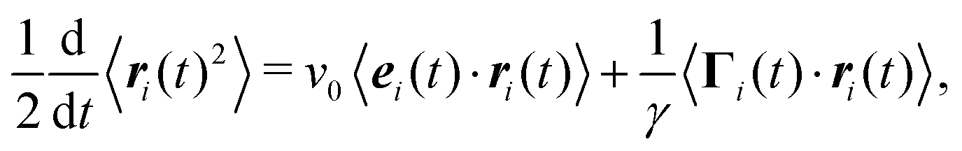
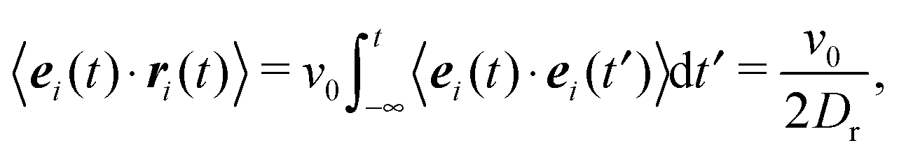
The equations of motion for a single, force-free particle in an infinite or periodic system follow from eqn (1) with Fi = 0. Multiplication of the remaining equation by ri(t) leads to| | 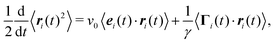 | (9) |
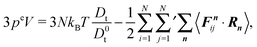
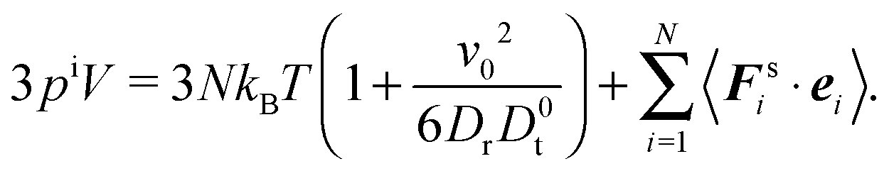
where 〈⋯〉 denotes the ensemble average. In the asymptotic limit t → ∞, the average on the left-hand side is the mean square displacement| | | 〈ri(t)2〉 = 〈ri(0)2〉 + 6Didtt | (10) |
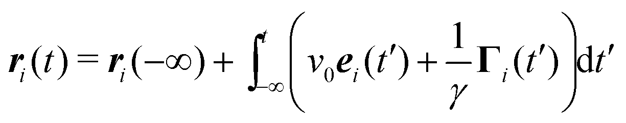
for the homogeneous and isotropic system. To evaluate the terms on the right-hand side, we use the formal solution| | 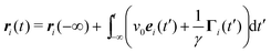 | (11) |
of eqn (1). Since ηi and Γi are independent stochastic processes, the terms on the right-hand side of eqn (9) reduce to| | 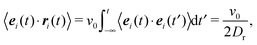 | (12) |
| |  | (13) |
Here, we use the correlation function (cf. Appendix B)| | | 〈ei(t)·ei(0)〉 = e−2Drt, | (14) |
and the definition| |  | (15) |
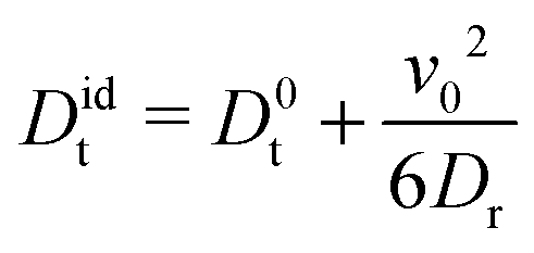
Hence, eqn (9) yields the diffusion coefficient| |  | (16) |
in the asymptotic limit t → ∞. This is a well-known relation for the mean square displacement of an active Brownian particle in three dimensions.1 However, we have derived the expression exploiting the virial theorem.34 More general, in d dimensions follows Didt = D0t + v02/d(d − 1)Dr.1 The expression has been confirmed experimentally for 2D synthetic microswimmers in ref. 41 and 42.
3.2 Confined particles – mean particle velocity
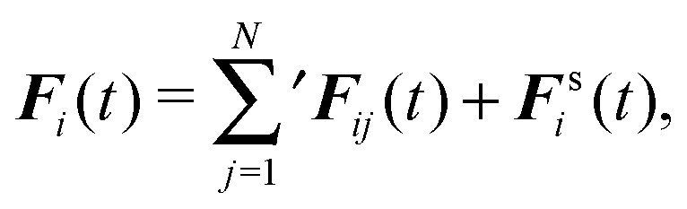
For ABPs confined in a volume with impenetrable walls, the force on particle i is| |  | (17) |
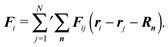
where the Fij = Fij(ri − rj) are pairwise interparticle forces and Fsi is the short-range repulsive force with the wall. We assume that the wall force points along the local surface normal n, i.e., Fsi = −Fsini, where ni = n(ri) points outward of the volume. The prime at the sum of eqn (17) indicates that the index j = i is excluded.
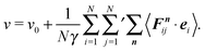
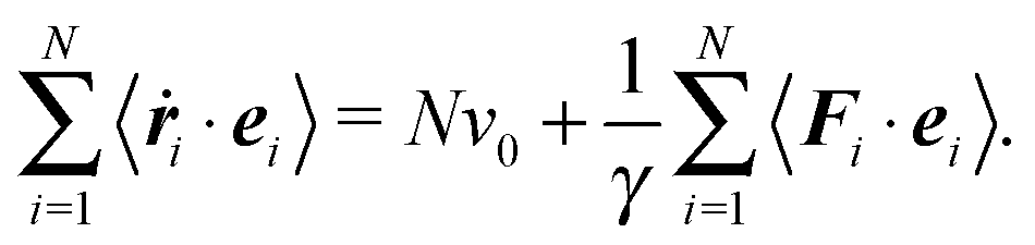
By multiplying eqn (1) with the orientation vector ei(t) and averaging over the random forces, we obtain
| |  | (18) |
The term 〈
ṙi·
ei〉 can be considered as the average of the particle velocity projected onto its propulsion direction, and hence,
| |  | (19) |
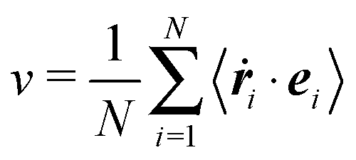
is the mean of the projected particle velocities in the interacting system.
23 In the following we will refer to this expression as mean particle velocity. With
eqn (17) and (18), the mean particle velocity can be expressed as
| | 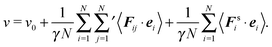 | (20) |
Aside from the wall term, a similar expression has been derived in
ref. 23. The pairwise interaction term can be written as
| |  | (21) |
As a consequence, we obtain a contribution to the velocity only when

.
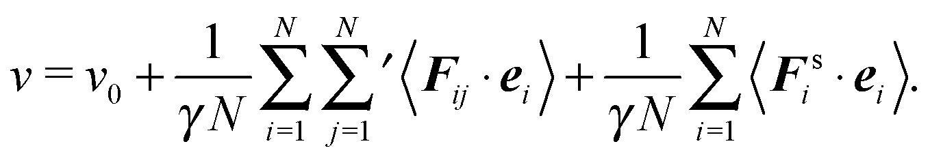
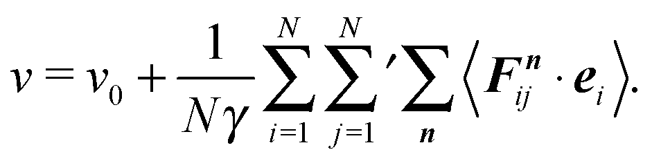
Evidently, v depends on the bare propulsion velocity v0, and interparticle and wall forces. However, only the projection of the force onto the respective propulsion direction appears. Thus, v reflects the magnitude of the mean particle velocity, but not the direction of motion.
The velocity perpendicular to a wall of a particle interacting with a wall is zero. Hence, the force 〈Fsi〉 of such a particle, averaged over the random force, is
for a dilute system. Thus, the wall force yields a contribution to the mean particle velocity as long as

. In the case of a dilute system, the mean velocity becomes
| |  | (23) |
Hence, the presence of walls reduces the velocity
v. This is in accordance with the considerations in
ref. 27 for anisotropic particles, but an extension of the calculations of
ref. 23 for spherical ABPs. Naturally, the velocity is zero for particles adsorbed at a wall and an orientation vector parallel to
n.
Generally, the average velocity of a particle along its propulsion direction, which is part time in the bulk, with probability Pbulk, and part time at the wall, with probability 1 − Pbulk, is
| | | vi = v0Pbulk + v0(1 − 〈(ei·ni)2〉)(1 − Pbulk). | (24) |
Thus, the distribution function of the angle between
ei and
ni is required, as well as the probability distribution to find a particle in the bulk to determine the average velocity
v. Naturally, the average in
eqn (23) can be calculated by the distribution function of the particle position and the propulsion orientation
ei, which follows from the respective Fokker–Planck equation under appropriate boundary conditions.
23,43
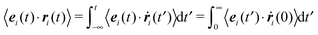
More general, multiplication of eqn (5) by the velocity ṙi(0) yields
| | | 〈ei(t)·ṙi(0)〉 = 〈ei(0)·ṙi(0)〉e−2Drt, | (25) |
within the Ito interpretation of the stochastic integral.
44–46 Then, averaging over all particles gives
| | 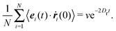 | (26) |
This relation describes the average decay of the correlation between the initial velocities
ṙi(0) and the time-dependent orientations
ei(
t). Not surprisingly, the correlation function decays exponentially, because the dynamics of the orientation
ei(
t) is independent of the particle position and any particle interaction.
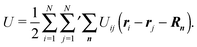
4 Virial formulation of pressure
The expression of the pressure depends on the boundary conditions. Here, we will discuss a system of ABPs confined in a cubic simulation box with either impenetrable walls or periodic boundary conditions.
4.1 Confined system
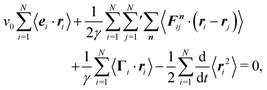
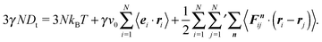
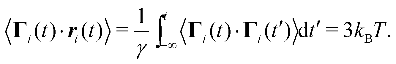
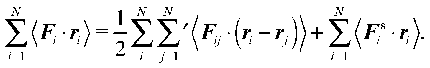
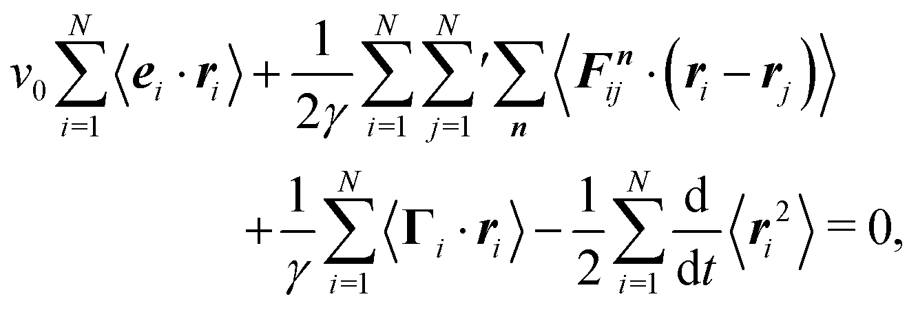
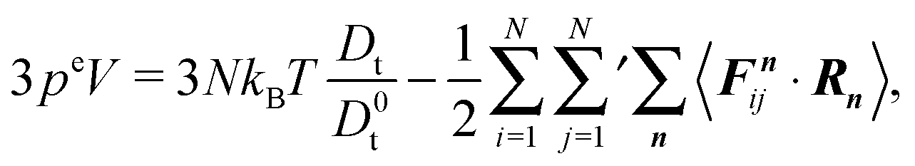
Multiplication of the equations of motion (1), with the forces (17), by ri(t) yields| | | γv0〈ei(t)·ri(t)〉 + 〈Γi(t)·ri(t)〉 + 〈Fi·ri〉 = 0, | (27) |
since the mean square displacement 〈ri(t)2〉 is limited in a confined system, and hence, its derivative vanishes in the stationary state. The force contribution can be written as| | 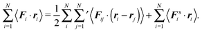 | (28) |
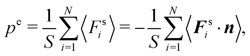
The first term on the right-hand side is the virial of the internal forces and the second term is that of the wall forces. The latter needs to be related to the pressure of the system, which is the major step in linking the mechanical (wall) pressure to bulk properties. The traditional derivation for equilibrium systems is briefly outlined in Appendix C. This derivation assumes a homogeneous pressure throughout the volume. In contrast, active systems can exhibit pressure inhomogeneities depending on the shape of the confining wall,15,47 and thus, the derivation does not apply in general. So far, there is no general derivation or proof of the equivalence of the external virial and the pressure; there may be no such universal equivalence, since there is no thermodynamic potential for an active system.
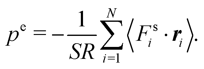
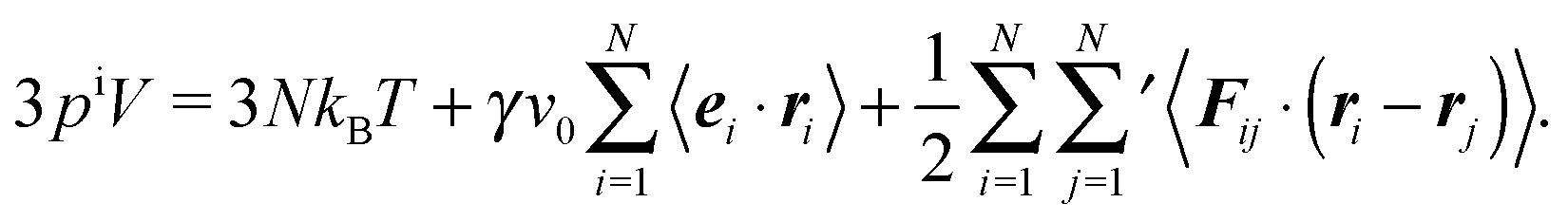
However, for special geometries, we can establish a relation between the wall forces and pressure. This particularly applies to cuboidal and spherical volumes. As shown in Appendix D, for such geometries the average wall pressure is given by
| |  | (29) |
where we introduce the external pressure
pe to indicate its origin by the external forces. As an important result, summation of
eqn (27) over all particles yields the relation between pressure and bulk properties
| | 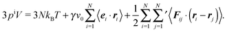 | (30) |
Naturally,
pi ≡
pe. However, we introduce the internal pressure
pi to stress the different nature in the pressure calculation by bulk properties. The first term on the right-hand side of
eqn (30) is the ideal-gas contribution to the pressure originating from the random stochastic forces
Γi (
eqn (13)). Without such forces, our system reduces to that considered in
ref. 13. The other two terms are the virial contributions by the active and interparticle forces. Following the nomenclature of
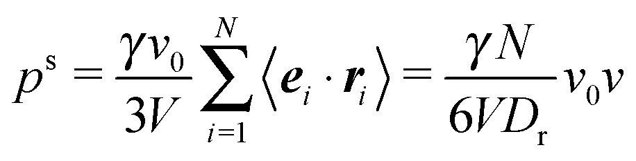
ref. 31, we denote the second term on the right-hand side as “swim virial”. It is a single-particle self-contribution to the pressure, in contrast to the virial contribution by the interparticle forces.
31 Hence, the swim virial shows a similarity with a contribution by an external field rather than interparticle forces.
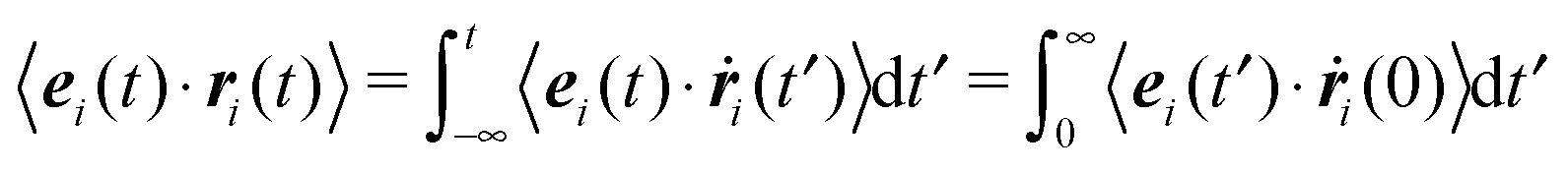
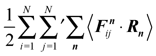
The contributions to the swim virial can be expressed as
| |  | (31) |
in the stationary state and with 〈
ri(−∞)·
ei(
t)〉 = 0. Together with
eqn (26),
eqn (30) can be expressed as
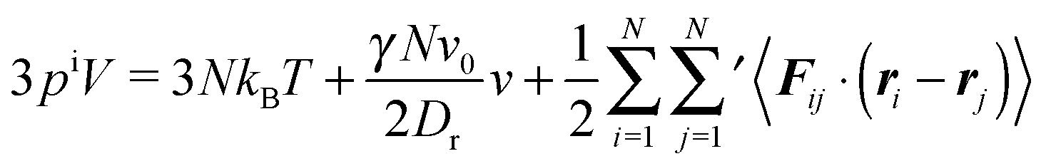
| |  | (32) |
in terms of the mean particle velocity
v (
eqn 20). A similar expression is obtained in
ref. 23, but in a very different way. However, in contrast to
ref. 23, our mean particle velocity (
eqn 20) comprises interparticle as well as wall contributions. Hence, the wall interactions are not only manifested in the pressure, but appear additionally in correlation functions,
i.e., 〈
ei(
t)·
ri(
t)〉. This is a major difference to passive systems, where
v0 and hence
v are zero.
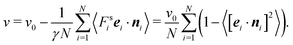
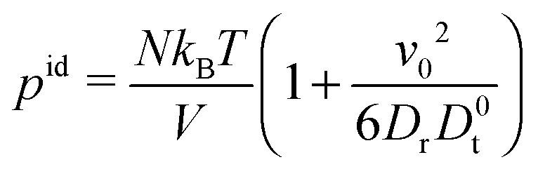
In the case of zero interparticle forces, the pressure in eqn (32) reduces to
| |  | (33) |
The first term on the right-hand side corresponds to the ideal (bulk) pressure
| |  | (34) |
of an active system.
23,31,39,47 The second term accounts for wall interactions, and is responsible for various phenomena such as wall accumulation.
13,15,43,47
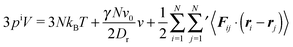
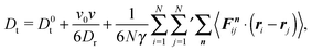
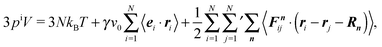
4.2 Periodic boundary conditions
In systems with periodic boundary conditions, there is no wall force Fs, but in addition to interactions between the N “real” particles, interactions with periodic images located at ri + Rn appear.
For a cubic simulation box, the vector Rn is given by
with
nα ∈
![[Doublestruck Z]](https://www.rsc.org/images/entities/char_e17d.gif)
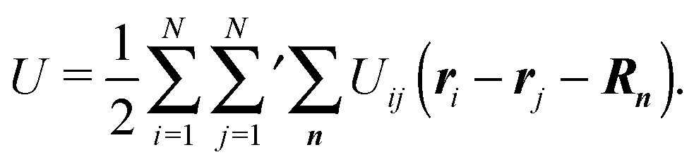
. The generalization to a rectangular noncubic box is straightforward. For a pair-wise potential
Uij, the potential energy is then given by
| |  | (36) |
In general, this involves infinitely many interactions.
35,48 Here, we will assume short-range interactions only. This limits the values
nα to
nα ± 1 for a particle in the primary box, which corresponds to an application of the minimum-image convention.
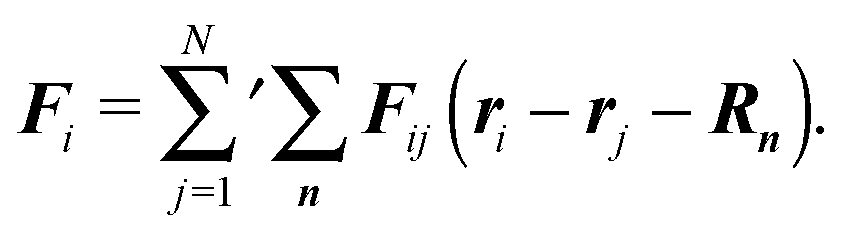
49 The forces in
eqn (1) are then given by
| |  | (37) |
Multiplication of
eqn (1) by
ri and summation over all particles lead to the relation
| |  | (38) |
with the abbreviation
Fij(
ri −
rj −
Rn) =
Fnij. By following the trajectories of the particles through the infinite system,
i.e., by not switching to a periodic image in the primary box, when a particle leaves that box, 〈
ri(
t)
2〉 is equal to the mean square displacement of
eqn (10), but with a translational diffusion coefficient
Dt of the interacting ABP system. Moreover,
eqn (13) applies and, hence,
| |  | (39) |
In the force-free case,
i.e.,
Fnij = 0, this relation is identical with
eqn (16). More general,
eqn (39) provides the self-diffusion coefficient of active particles in a periodic system interacting by pair-wise forces. Exploiting
eqn (26) and (31), the swim virial can be expressed by the mean particle velocity
v, and the diffusion coefficient becomes
| |  | (40) |
with the mean particle velocity in a periodic system
| |  | (41) |
After insertion of velocity
v,
eqn (40) provides three contributions to the diffusion coefficient: (i) the diffusion coefficient,
eqn (16), of non-interacting active Brownian particles, (ii) a contribution due to correlations between the forces
Fnij and the orientations
ei, and (iii) a contribution from the virial of the inter-particle forces. This clearly reflects the explicit dependence of the diffusion coefficient on the orientational dynamics of the particles.
In contrast to confined systems, the multiplication of the equations of motion by the particle positions does not directly provide an expression for the pressure of a periodic system. Here, additional steps are necessary. To derive an expression for the pressure, we subtract the term
| |  | (42) |
from both sides of
eqn (39). Then, we are able to define external (
pe) and internal (
pi) pressures of the periodic system according to
| |  | (43) |
| |  | (44) |
as for passive systems in
ref. 35–37. Naturally, both expressions yield the same pressure value,
i.e.,
pe ≡
pi.
For notational convenience, we write the expressions for the pressure as
with the following contributions according to
eqn (43) and (44)
• ideal gas pressure
| |  | (47) |
• swim pressure—specific for active systems
| | 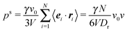 | (48) |
• internal pressure by interparticle forces—contains active contributions
| | 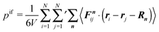 | (49) |
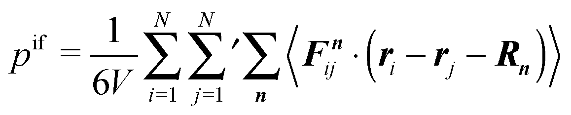
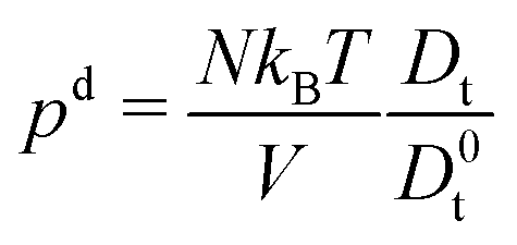
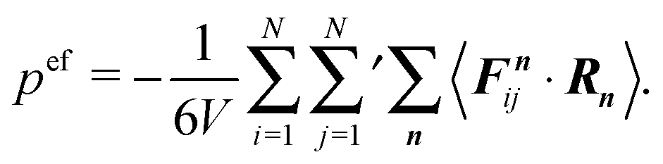
• pressure by diffusion—contains active contributions via swim pressure and interparticle forces
| |  | (50) |
• external pressure by interparticle forces—contains active contributions
| |  | (51) |
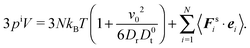
The expressions in eqn (43) and (44) are extensions of those of a conservative passive system, where Dt = 0 and v0 = 0, with a similar definition of external and internal pressures.35,50 For both cases, the definitions appear ad hoc. Note that for a passive system typically Newton's equations of motion are considered. However, for the passive system, the expression for the internal pressure can be derived from the free energy,51 as illustrated in the appendix of ref. 50, which underlines the usefulness and correctness of the applied procedure for passive systems. The similarity between the internal pressure expressions eqn (30) and (44) for the confined and periodic systems, respectively, supports the adequateness of the applied procedure in the pressure calculation.
The individual terms can be understood as follows.
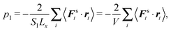
External pressure pe.
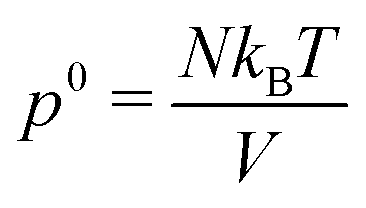
The pressure contribution pef accounts formally for the forces across faces of the periodic system, similar to the expression (29) of a confined system. There is only a contribution for non-zero vectors Rn, i.e., for interactions between real and image particles.35 The diffusive dynamics yields the pressure contribution pd ∼ Dt/D0t. This term is not present in a conservative passive system and is a consequence of the stochastic forces Γi.35–37 For passive, non-interacting particles, i.e., v0 = 0 and U of eqn (36) is zero, Dt = D0t and the pressure reduces to the ideal gas expression pe = p0. For non-interacting but active systems, Dt is given by eqn (16) and pe = pid (eqn (34)).
Internal pressure pi.
The internal pressure comprises the ideal gas contribution p0, the swim pressure ps due to activity, and the contribution pif by the pairwise interactions in the system within the minimum-image convention. As for the virial of the confined system (32), the swim pressure pseqn (48) can be expressed by the mean particle velocity v (eqn (41)). The forces Fnij can be strongly correlated with the propagation direction ei, specifically when the system phase separates as in ref. 21. For non-interacting particles or at very low concentrations, the contribution of the intermolecular forces vanishes and the pressure is given by eqn (34).
There are various similarities between the expressions for the pressure of a confined and a periodic system. Formally, eqn (32) and (44) are similar. However, specifically the meaning of the mean particle velocity v is very different. The presence of the wall term in eqn (20) can lead to wall-induced phenomena, which are not present in periodic systems. Hence, results of simulations of periodic and confined active systems are not necessarily identical.
5 Simulation results
Simulations of active Brownian spheres with periodic boundary conditions (cf. Section 2) reveal an intriguing phase behavior and a highly collective dynamics, as discussed in ref. 21 for three dimensional systems. At low concentrations, the ABPs exhibit a uniform gas-like phase. However, above a critical, Péclet-number-dependent concentration, the isotropic system phase separates into a dilute, gas-like phase, and a dense, liquid-like phase.14,21Fig. 1 illustrates the phase diagram for the considered concentrations and Péclet numbers, redrawn from the simulation data of ref. 21. Above Pe ≈ 30, we find a wide range of concentrations, over which the system phase separates. In the simulations, the phase separation of the ABPs into a dense liquid phase and a dilute gas phase is clearly reflected in the probability distribution of the local ABP packing fraction, which we determine by a Voronoi construction. Below a critical density, the probability distribution is unimodal and the system is homogeneous. While approaching the critical density with increasing packing fraction, the probability distribution becomes bimodal and the system inhomogeneous. Moreover, the morphological transformations are reflected in geometric characteristics, such as the surface area, integrated mean curvature, and the Euler characteristics, as discussed in detail in ref. 21.
 |
| | Fig. 1 Illustration of the phase diagram of active Brownian particles in terms of the Péclet number Pe and the packing fraction ϕ. Symbols correspond to the Péclet numbers for which the pressure is calculated. The shaded areas indicate the liquid–gas (light green) and the crystal–gas (light yellow) coexistence regimes. Further details can be found in ref. 21. | |
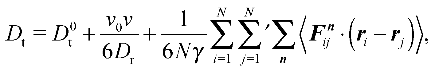
As is evident from eqn (43) and (44), the diffusion coefficient explicitly appears in the expressions of the pressure. Hence, we address the dynamics of the ABPs in terms of the diffusion coefficient in the following. Subsequently, we discuss the dependence of the pressure and its individual contributions on the Péclet number and concentration.
5.1 Diffusion coefficient of ABPs
We determine the diffusion coefficient of the ABPs by the Einstein relation, i.e., we calculated the particle mean square displacement and extracted the translational coefficient Dt from the linear long-time behavior. Fig. 2 displays the obtained values as a function of the packing fraction for various Péclet numbers. For small packing fractions (ϕ ≲ 0.3), Dt/Didt decreases linearly with increasing concentration. The decay is reasonably well described by the theoretically expected relation 1 − 2ϕ for colloids in solution.52 However, a better agreement is obtained for the relation 1 − 2.2ϕ, i.e., a 10% larger prefactor. Remarkably, the decrease of Dt for ϕ ≲ 0.3 is essentially independent of the activity. Significant deviations between the individual curves are visible for higher concentrations and larger Péclet numbers, where a phase separation appears. At the critical concentration, the diffusion coefficients for Pe > 30 exhibit a rapid change to smaller values. A further increase in concentration implies a further slowdown of the dynamics. Interestingly, at high concentrations, the larger Péclet number ABPs diffuse faster than those with a small Pe. We attribute this observation to collective effects of the fluids exhibiting swirl- and jet-like structures.21 Another reason might be an activity induced fluidization, since the glass transition is shifted to larger packing fractions.22
 |
| | Fig. 2 Translational diffusion coefficients of ABPs for the Péclet numbers Pe = 9.8 (purple), 29.5 (olive), 44.3 (green), 59.0 (blue), and 295.0 (red). The values are normalized by the respective diffusion coefficients (16) of an individual ABP. The inset shows the same data on linear scales. The solid line (black) indicates the dependence Dt/Didt = 1 − 2ϕ. | |
5.2 Pressure of ABPs
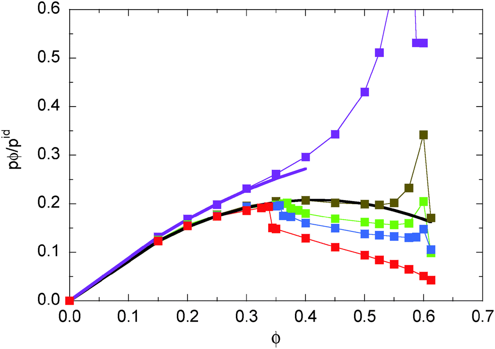
Fig. 3 displays the density dependence of the total pressure p ≡ pe ≡ pi for the considered Péclet numbers. We normalize the pressure by the ideal gas value (34) and multiply by the packing fraction ϕ in order to retain the linear density dependence. As expected, both eqn (45) and (46) yield the same pressure values. We observe a pronounced dependence of the pressure on the Péclet number. Note that the pressure for the largest Péclet number is highest, because pid ∼ Pe2 for Pe ≫ 1. For small Pe, the pressure increases with increasing ϕ. However, already for Pe = 29.5, we obtain a strongly nonmonotonic concentration dependence, where the pressure decreases again for ϕ ≳ 0.35. A similar behavior has already been obtained in ref. 13, 23 and 31. In ref. 31, the decreasing pressure at high concentrations is attributed to cluster formation of the ABPs. For ABPs with Péclet numbers well in the phase separating region, we find a jump of the pressure at the critical packing fraction. This behavior has not been observed before, most likely because only smaller Péclet numbers have been considered. Such a pressure jump seems not to be present for Pe = 29.5, but the Pećlet number is close to the binodal (cf.Fig. 1) and a clear phase separation is difficult to detect in simulations.
 |
| | Fig. 3 Pressure in systems of ABPs for the Péclet numbers Pe = 9.8 (purple), 29.5 (olive), 44.3 (green), 59.0 (blue), and 295.0 (red). The values are normalized by the pressure pid (34) of individual ABPs at the same Péclet number. The black line indicates the dependence pϕ/pid = ϕ(1 − 1.2ϕ), and the purple line the relation pϕ/pid = ϕ(1 − 0.8ϕ). | |
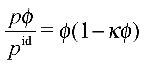
Interestingly, all the pressure curves exhibit a remarkably similar behavior for Pe ≥ 29.5 and ϕ < 0.35 and can very well be fitted by the density dependence
| |  | (52) |
in this regime, with
κ ≈ 1.2, as indicated in
Fig. 3. For smaller Pe = 9.8, we find
κ ≈ 0.8. Hence, in any case the pressure increases linearly for
ϕ ≪ 1, as expected, and exhibits quadratic corrections for larger concentrations, which depend on the swimming velocity or the Péclet number. In
ref. 31, the nonequilibrium virial equation of state
| | | p = pid[1 − (1 − 3/2Pe)ϕ] | (53) |
is proposed, adopted to our definition of the Péclet number, and
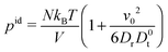
pid =
NkBT(1 − Pe
2/2)/
V. This relation applies only within a certain range of Pe values. It certainly accounts for the increase of the prefactor of
ϕ with increasing Pe, but the asymptotic value for Pe ≫ 1 does not agree with our simulation results. However, our simulation results for Pe = 9.8 are reasonably well described by
eqn (53) at small concentrations.
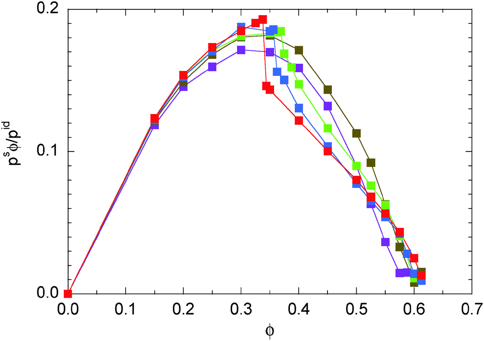
The nonlinear concentration dependence of eqn (52) with a positive κ yields a negative second-virial coefficient B2 = −πσ3κ/6. In classical thermodynamics, a negative B2 suggests the possibility of a gas–liquid phase transition.31 For the ABPs, the negative B2 definitely indicates large concentration fluctuations, which increase with increasing Péclet number. However, in the light of our simulation results, it seems that a phase transition is also associated with a pressure jump at the critical concentration. This is more clearly expressed by the swim pressure ps displayed in Fig. 4. Only for Pe > 29.5, we find a pressure jump and a phase transition.
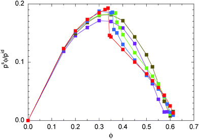 |
| | Fig. 4 Swim pressure eqn (48) in systems of ABPs for the Péclet numbers Pe = 9.8 (purple), 29.5 (olive), 44.3 (green), 59.0 (blue), and 295.0 (red). The values are normalized by the pressure pid(34) of individual ABPs at the same Péclet number. | |
Fig. 5 illustrates the contributions of the individual terms of eqn (48)–(51) to the total pressure for the Péclet numbers Pe = 9.8 and Pe = 295. At small Pe = 9.8 (see Fig. 5(a)), the terms ps and pd decrease monotonically with increasing concentration and approach zero at large ϕ. For pd, this is easily understood by the slowdown of the diffusive dynamics due to an increase in frequency of particle encountered with increasing density. The pressure pd is given by
| |  | (54) |
in terms of the ideal gas and the swim pressure. As for a passive system, the last term on the right-hand side of this equation is smaller than zero, and hence,
ps >
pd −
p0. The equation also shows that the swim pressure is generally different from
pd and, hence, is not simply related to the diffusive behavior of the ABPs. As far as the force contributions
pef and
pif are concerned, they monotonically increase with
ϕ for Pe = 9.8, until the ABPs undergo a phase transition and form a crystalline structure. The gradual increase of the number of interacting colloids with increasing concentration leads to a systematic increase of the pressure contribution by pairwise force. The ratio
p/
pid decreases initially (
ϕ < 0.4) due to the slowdown of the diffusive dynamics, but at large
ϕ, the contributions
pef and
pif dominate and the respective pressure increases with concentration similar to that of a passive system. For Pe = 9.8,
p is essentially equal to
pef for
ϕ > 0.5.
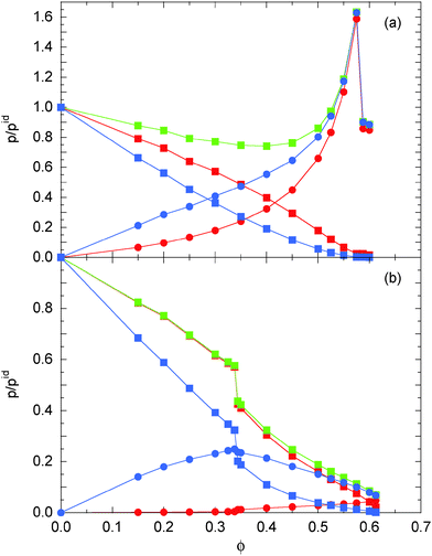 |
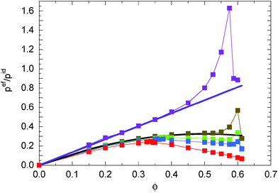
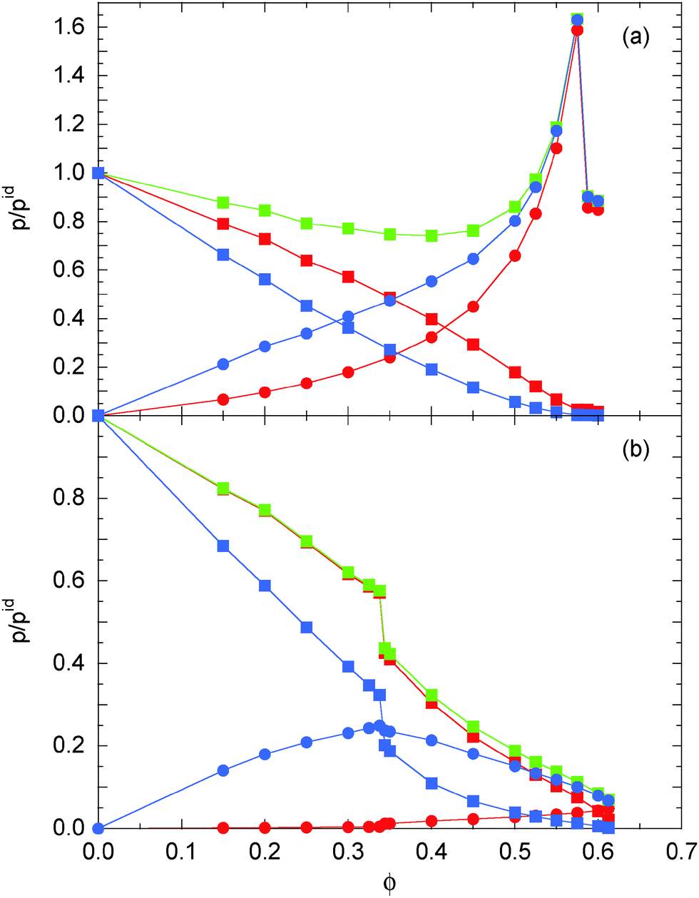
| | Fig. 5 Pressure and its individual contributions of ABPs for the Péclet number (a) Pe = 9.8 and (b) Pe = 295.0. The values are normalized by the pressure pid(34) of individual ABPs at the same Péclet number. The green symbols indicate the total pressure eqn (45) and (46). The red symbols correspond to internal pressure components ps ( ) and pif ( ) and pif ( ) of eqn (48) and (49), respectively. The blue symbols indicate the pressure components pd ( ) of eqn (48) and (49), respectively. The blue symbols indicate the pressure components pd ( ) and pef ( ) and pef ( ) of eqn (50) and (51), respectively. ) of eqn (50) and (51), respectively. | |
The relevance of the individual contributions changes with increasing Péclet number. For Pe = 295 (see Fig. 5(b)), pd and ps still decrease monotonically with increasing ϕ. However, the total pressure is essentially identical with ps, i.e., p is dominated and determined by the swim pressure. The contribution pif due to interparticle interactions is very small and is only relevant at high concentrations. The pressure pef increase for small concentrations passes through a maximum and decreases again for large ϕ. This nonmonotonic behavior is very different from that at low-Péclet numbers. The jumps in ps and pd reflect the phase transition at a critical density ϕc.21 Note that the critical density depends on the Péclet number.
Aside from absolute values, the density dependence of the various pressure components is rather similar for densities below the critical density ϕc ≈ 0.35. In any case, the pressure is dominated by the active contribution as expressed and reflected in the diffusion coefficient. Above ϕc, however, the contribution by the inter-particle forces dominates for Pe = 9.8, whereas p is still determined by ps for Pe = 295. Here, the contribution of ps exceeds that of pif by far, although the latter increases also with the Péclet number as shown in Fig. 6, but ps ∼ Pe2 at small ϕ and outweighs the growth of pif. Two effects contribute to the decrease of the overall pressure. The diffusion coefficient decreases with increasing concentration due to an increasing number of particle–particle encounters. However, pd decreases faster than ps. Viarelation (54), we see that this faster decrease is compensated by an increase in the contribution by the interparticle forces.
 |
| | Fig. 6 Contribution of the interparticle force (eqn (49)) to the internal pressure of ABPs for the Péclet numbers Pe = 9.8 (purple), 29.5 (olive), 44.3 (green), 59.0 (blue), and 295.0 (red). The solid line (black) indicates the dependence pif ∼ e6ϕ. | |
Looking at the swim pressure ps (cf.eqn (41)), it evidently decreases because the correlations between the forces and the orientations ei decrease with increasing concentration. Here, an important aspect is the appearance of collective effects of the ABPs, specifically for ϕ > ϕc.21 Collective effects lead to a preferential parallel alignment of certain nearby ABPs. As indicated in eqn (21), such an alignment reduces the force-propulsion-direction correlations, and hence, the pressure.
As indicated before, the force contribution to the internal pressure pif depends roughly linearly on Pe, as illustrated in Fig. 6. Remarkably, pif exhibits an exponential dependence on density, namely pif ∼ exp(6ϕ), over a wide range of concentrations for Péclet numbers in the one-phase regime, and up to the critical value ϕc for Péclet numbers where a phase transition appears. Additionally, the forces exhibit a rapid increase at the critical density. We did not analyse in detail whether a jump appears or if pif is smooth and a gradual but rapid increase occurs, as might be expected from the data for Pe = 44.3.
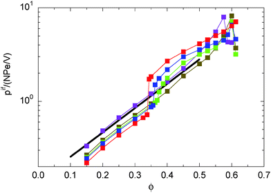
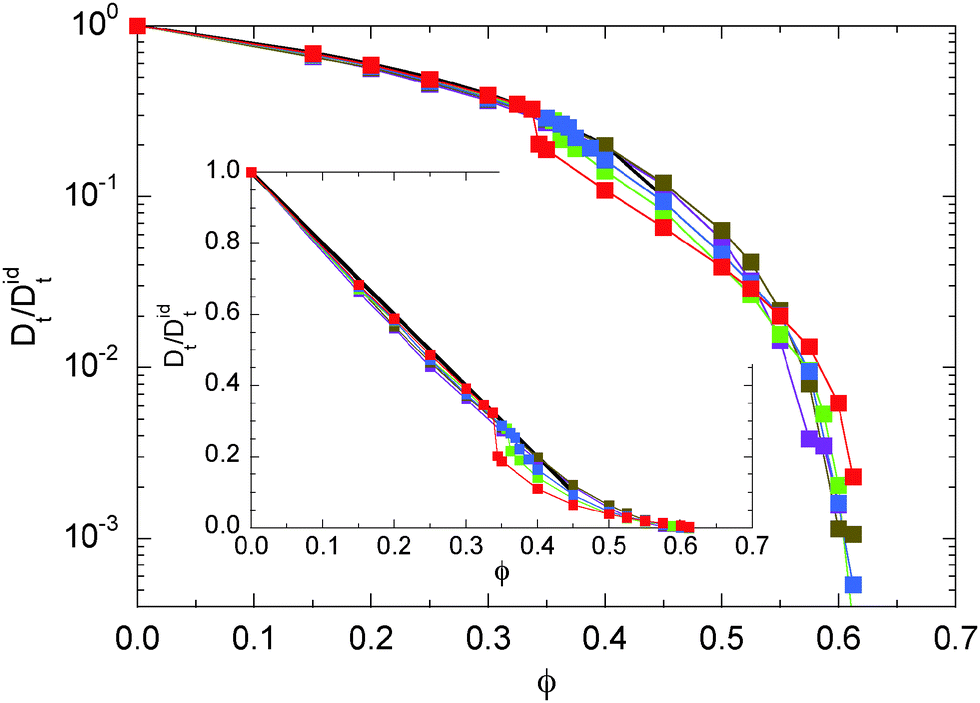
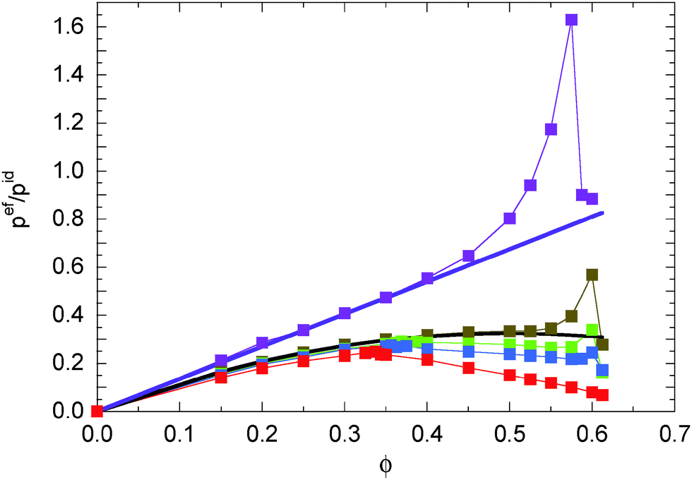
Fig. 7 displays the contributions of the internal forces (eqn (51)) to the external pressure (eqn (46)). The general shape of the curves is comparable to that of the scaled pressure pϕ/pid. Compared to the latter, pef exhibits the stronger density dependence pef ∼ ϕ2 for ϕ ≪ 1. However, compared to pif, the density dependence is weak. Quantitatively, it can be described as pef/pid = ![[small kappa, Greek, circumflex]](https://www.rsc.org/images/entities/i_char_e109.gif) ϕ(1 − ϕ) with ≈ 1.35 over a wide range of Péclet numbers 9 < Pe ≲ 30. With increasing Pe, decreases slightly and we find ≈ 1.1 for Pe = 295.
ϕ(1 − ϕ) with ≈ 1.35 over a wide range of Péclet numbers 9 < Pe ≲ 30. With increasing Pe, decreases slightly and we find ≈ 1.1 for Pe = 295.
 |
| | Fig. 7 Contribution of the interparticle force (eqn (51)) to the external pressure of ABPs for the Péclet numbers Pe = 9.8 (purple), 29.5 (olive), 44.3 (green), 59.0 (blue), and 295.0 (red). The solid lines indicate the dependencies pef/pid ≈ 1.35ϕ (purple) and pef/pid ≈ 1.3ϕ(1 − ϕ) (black). | |
6 Summary and conclusions
We have presented theoretical and simulation results for the pressure in systems of spherical active Brownian particles in three dimensions. In the first step, we have shown that the mechanical pressure as force per area can be expressed via the virial by bulk properties for particular geometries, especially a cuboid volume as typically used in computer simulations. Subsequently, we have derived expressions for the pressure via the virial theorem of systems confined in cuboidal volumes or with periodic boundary conditions. For the latter, two equivalent expressions are derived, denoted as internal and external pressures, respectively. As a novel aspect, we considered overdamped equations of motion for active systems in the presence of a Gaussian and Markovian white-noise source. The latter gives rise to a thermal diffusive dynamics for the translational motion and yields the ideal-gas contribution to the pressure.
The activity of the Brownian particles yields distinct contributions to the respective expressions of the pressure. The external pressure explicitly comprises the effective diffusion coefficient of the active particles. The internal pressure contains a term, which is related to the product of the bare propulsion velocity of an ABP and their mean velocity. The latter is determined by the interactions with surrounding ABPs and reduces to the bare velocity at infinite dilution. Similar expressions have been derived in ref. 13, 23 and 31.
Our simulations of ABPs in systems with three-dimensional periodic boundary conditions show that the total pressure increases first with concentration and decreases then again at higher concentrations for Péclet numbers exceeding a ceratin value, in agreement with previous studies.13,31 Thereby, the pressure exhibits a van der Waals-like pressure–concentration curve. This shape clearly reflects collective effects, however, it does not necessarily indicate a phase transition. In the case of a phase transition, we find a rapid and apparently discontinuous reduction of the pressure at the phase-separation density.
Quantitatively, the density dependence of the pressure is well described by the relation p ∼ ϕ(1 − κϕ), where the range over which the formula applies and κ depend on the Péclet number. For Pe ≈ 10, we find κ ≈ 0.8. For Péclet numbers in the vicinity and above Pec, all the considered curves are well described with κ ≈ 1.2. Generally speaking, our κ values extracted from the simulations are in the vicinity of the value κ = 1 as proposed in ref. 31.
Considering the various contributions to the pressure individually, we find that the internal pressure is dominated by the contribution from activity for Pe > Pec, in particular for ϕ < ϕc. For Péclet numbers larger than the critical value, there is significant contribution from the interparticle forces of eqn (41). This contribution decreases with increasing Péclet number, since the swim pressure increases quadratically with the Péclet number and the pressure due to interparticle force linearly. However, for moderate Pe, the exponential increase of pif with concentration outweighes the Péclet-number dependence.
In summary, the pressure of an active system exhibits distinctive differences to a passive system during an activity-induced transition from a (dilute) fluid to a system with a coexisting gas and a dense liquid phase. While the pressure of a passive system remains unchanged during the phase transition, our simulations of an active system yield a rapid decrease of the pressure for densities in the vicinity of the phase-transition density. Thereby, the pressure change becomes more pronounced with increasing Péclet number. Hence, evaluation of the pressure, specifically the swim pressure, provides valuable insight into the phase behavior of active systems.
Appendix A Rotational equation of motion
Eqn (5) is a stochastic equation with multiplicative noise. The Fokker–Planck equation, which yields the correct equilibrium distribution function, follows with the white noise in the Stratonovich calculus.44,46,53
For the numerical integration of the equations of motion (5), an Ito representation is more desirable. Introducing spherical coordinates according to
| |  | (55) |
(here, we consider a particular particle and skip the index i), alternatively the stochastic differential equation can be considered
and yields the same Fokker–Planck equation for the generalized coordinates
φ and
ϑ.
46 Thereby, the equations of motion of the angles are
| |  | (57) |
| |  | (58) |
with additive noise. The unit vectors
eξ,
ξ ∈ {
φ,
ϑ}, follow by differentiation
eξ ∼ ∂
e/∂
ξ and normalization. The
ηξ are again Gaussian and Markovian random processes with the moments
| | | 〈ηξ(t)ηξ′(t′)〉 = 2Drδξξ′δ(t − t′). | (59) |
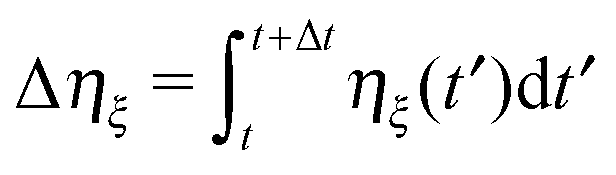
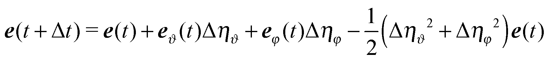
For simulation, eqn (56) has to be discretized. Integration, iteration, and usage of eqn (57) and (58) yield the difference equation
| | | e(t + Δt) = e(t) + eϑ(t)Δηϑ + eφ(t)Δηφ − 2Dre(t)Δt. | (60) |
The Δ
ηξ are defined as
| |  | (61) |
and are Gaussian random numbers with the first two moments
| | | 〈ΔηξΔηξ′〉 = 2Drδξξ′Δt. | (62) |
This is easily shown with the help of
eqn (59).
45 As common for the Ito calculus, we replaced the values Δ
ηξ2 by their averages 2
DrΔ
t in
eqn (60).
45,46
For practical reasons, it is more convenient to apply the following integration scheme. An “estimate” e′(t + Δt) is obtained via
| | | e′(t + Δt) = e(t) + eϑ(t)Δηϑ + eφ(t)Δηφ. | (63) |
This new orientation vector is no longer normalized. Normalization yields
e(
t + Δ
t) =
e′(
t + Δ
t)/|
e′(
t + Δ
t)|, where |
e′(
t + Δ
t)|
2 =
e′(
t + Δ
t)·
e′(
t + Δ
t) = 1 + Δ
ηϑ2 + Δ
ηϑ2. Since Δ
ηφ2 ∼ Δ
t, we obtain for
DrΔ
t ≪ 1
| |  | (64) |
up to order Δ
t3/2. Upon replacement of Δ
ηξ2 by its average, we obtain the desired
eqn (60).
B Orientational vector correlation function
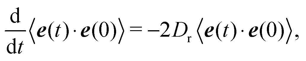
The autocorrelation function of the orientational vector is conveniently obtained from eqn (5) for an infinitesimal time interval dt, i.e., the equation| | | de = e(t) × dη(t) − 2Dredt | (65) |
within the Ito calculus. Multiplication with e(0) and averaging yields| | | 〈de(t)·e(0)〉 = 〈[e(t) × dη(t)]·e(0)〉 − 2Dr〈e(t)·e(0)〉dt. | (66) |
Since e(t) is a nonanticipating function,45 the average over the stochastic-force term vanishes, and we get
which gives
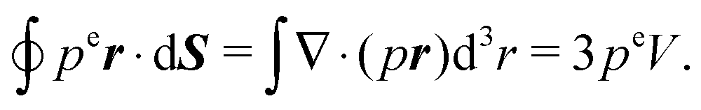
C Virial and pressure in equilibrium systems
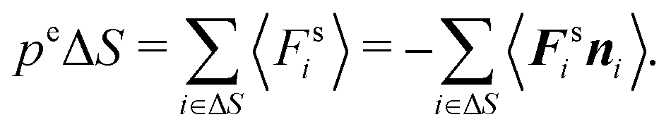
To relate the external virial with the pressure for an equilibrium system, we consider a surface element ΔS and the forces exerted on that surface element  . The pressure pe at the surface element is
| |  | (67) |
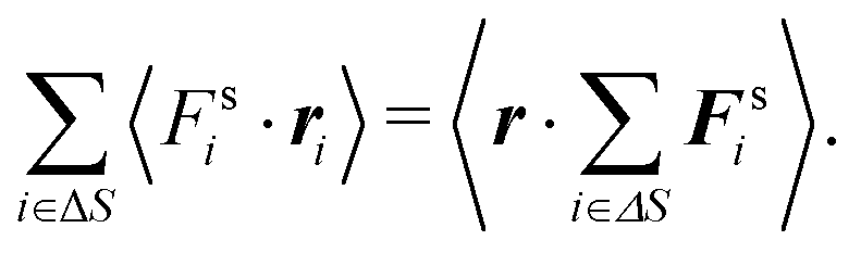
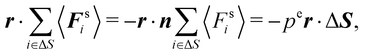
On the other hand, the external virial reads as| |  | (68) |
Since the surface element is small, the vector ri is essentially the same for all particles interacting with ΔS and can be replaced by the vector r of that element. The same applies to the normal ni, i.e., ni = n, where n is the local normal at ΔS. With eqn (68) and the mechanical pressure, we then obtain| |  | (69) |
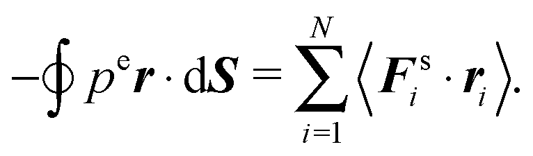
with ΔS = nΔS. Integration over the whole surface gives| |  | (70) |
Using the Gauss theorem, the surface integral turns into a volume integral, i.e.,| | 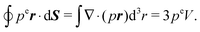 | (71) |
For the last equality, we assume that the pressure is isotropic and homogeneous. Hence,34| | 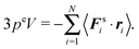 | (72) |
D Virial and pressure of active particles
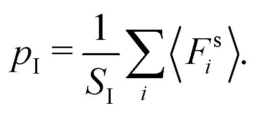
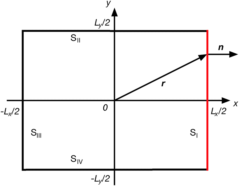
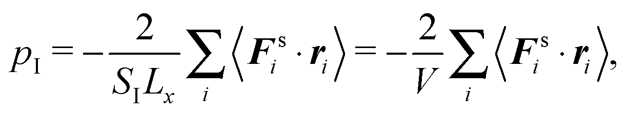
D.1 Cuboidal confinement
We consider particles confined in a cuboidal volume of dimensions Lx × Ly × Lz, with the reference frame located in its center (cf.Fig. 8). The total mechanical pressure is given by the average over the six surfaces, i.e., pe = (pI + pII + ⋯ + pVI)/6. For surface SI, the mechanical pressure is| | 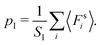 | (73) |
 |
| | Fig. 8 Cross section of a cuboid for the calculation of mechanical pressure. | |
Since n·ri = Lx/2 for any point on the surface, we introduce unity, i.e., n·ri/(Lx/2) = 1 and obtain
| |  | (74) |
with
Fsi = −
Fsin. Hence, the pressure is given by
| |  | (75) |
as for an equilibrium system. The derivation of this relation is independent of the choice of the Cartesian reference frame. At least, as long as the axis unit-vectors are normal to the surfaces.
D.2 Spherical confinement
For a sphere of radius R with the reference frame in its center, the pressure is| | 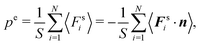 | (76) |
where S = 4πR2. For every point on the surface applies ri = Rn, hence,| |  | (77) |
With SR = 4πR3 = 3V, we again find relation (75).
Acknowledgements
We gratefully acknowledge support from the DFG within the priority program SPP 1726 “Microswimmers”.
References
- J. Elgeti, R. G. Winkler and G. Gompper, Rep. Prog. Phys., 2015, 78, 056601 CrossRef CAS PubMed.
- T. Vicsek and A. Zafeiris, Phys. Rep., 2012, 517, 71 CrossRef PubMed.
- M. F. Copeland and D. B. Weibel, Soft Matter, 2009, 5, 1174 RSC.
- N. C. Darnton, L. Turner, S. Rojevsky and H. C. Berg, Biophys. J., 2010, 98, 2082 CrossRef CAS PubMed.
- D. B. Kearns, Nat. Rev. Microbiol., 2010, 8, 634–644 CrossRef CAS PubMed.
- K. Drescher, J. Dunkel, L. H. Cisneros, S. Ganguly and R. E. Goldstein, Proc. Natl. Acad. Sci. U. S. A., 2011, 10940, 108 Search PubMed.
- J. D. Partridge and R. M. Harshey, J. Bacteriol., 2013, 195, 909 CrossRef CAS PubMed.
- J. Bialké, T. Speck and H. Löwen, Phys. Rev. Lett., 2012, 108, 168301 CrossRef.
- I. Buttinoni, J. Bialké, F. Kümmel, H. Löwen, C. Bechinger and T. Speck, Phys. Rev. Lett., 2013, 110, 238301 CrossRef.
- B. M. Mognetti, A. Šarić, S. Angioletti-Uberti, A. Cacciuto, C. Valeriani and D. Frenkel, Phys. Rev. Lett., 2013, 111, 245702 CrossRef CAS.
- I. Theurkauff, C. Cottin-Bizonne, J. Palacci, C. Ybert and L. Bocquet, Phys. Rev. Lett., 2012, 108, 268303 CrossRef CAS.
- Y. Fily, S. Henkes and M. C. Marchetti, Soft Matter, 2014, 10, 2132 RSC.
- X. Yang, M. L. Manning and M. C. Marchetti, Soft Matter, 2014, 10, 6477 RSC.
- J. Stenhammar, D. Marenduzzo, R. J. Allen and M. E. Cates, Soft Matter, 2014, 10, 1489 RSC.
- Y. Fily, A. Baskaran and M. F. Hagan, Soft Matter, 2014, 10, 5609 RSC.
- G. S. Redner, M. F. Hagan and A. Baskaran, Phys. Rev. Lett., 2013, 110, 055701 CrossRef.
- Y. Fily and M. C. Marchetti, Phys. Rev. Lett., 2012, 108, 235702 CrossRef.
- R. Großmann, L. Schimansky-Geier and P. Romanczuk, New J. Phys., 2012, 14, 073033 CrossRef.
- V. Lobaskin and M. Romenskyy, Phys. Rev. E: Stat., Nonlinear, Soft Matter Phys., 2013, 87, 052135 CrossRef.
- A. Zöttl and H. Stark, Phys. Rev. Lett., 2014, 112, 118101 CrossRef.
- A. Wysocki, R. G. Winkler and G. Gompper, EPL, 2014, 105, 48004 CrossRef.
- R. Ni, M. A. Cohen Stuart and M. Dijkstra, Nat. Commun., 2013, 4, 2704 Search PubMed.
- A. P. Solon, J. Stenhammar, R. Wittkowski, M. Kardar, Y. Kafri, M. E. Cates and J. Tailleur, Phys. Rev. Lett., 2015, 114, 198301 CrossRef.
- J. Bialké, H. Löwen and T. Speck, EPL, 2013, 103, 30008 CrossRef.
- J. Stenhammar, A. Tiribocchi, R. J. Allen, D. Marenduzzo and M. E. Cates, Phys. Rev. Lett., 2013, 111, 145702 CrossRef.
- R. Wittkowski, A. Tiribocchi, J. Stenhammar, R. J. Allen, D. Marenduzzo and M. E. Cates, Nat. Commun., 2014, 5, 4351 CAS.
- A. P. Solon, Y. Fily, A. Baskaran, M. E. Cates, Y. Kafri, M. Kardar and J. Tailleur, Nat. Phys., 2015 DOI:10.1038/nphys3377.
- S. C. Takatori and J. F. Brady, Phys. Rev. E: Stat., Nonlinear, Soft Matter Phys., 2015, 91, 032117 CrossRef CAS.
- T. F. F. Farage, P. Krinninger and J. M. Brader, Phys. Rev. E: Stat., Nonlinear, Soft Matter Phys., 2015, 91, 042310 CrossRef CAS.
- C. Maggi, U. M. B. Marconi, N. Gnan and R. Di Leonardo, Sci. Rep., 2015, 5, 10742 CrossRef PubMed.
- S. C. Takatori, W. Yan and J. F. Brady, Phys. Rev. Lett., 2014, 113, 028103 CrossRef CAS.
- F. Ginot, I. Theurkauff, D. Levis, C. Ybert, L. Bocquet, L. Berthier and C. Cottin-Bizonne, Phys. Rev. X, 2015, 5, 011004 Search PubMed.
- E. Bertin, Physics, 2015, 8, 44 CrossRef.
-
R. Becker, Theory of Heat, Springer Verlag, Berlin, 1967 Search PubMed.
- R. G. Winkler, H. Morawitz and D. Y. Yoon, Mol. Phys., 1992, 75, 669 CrossRef CAS PubMed.
- R. G. Winkler and R. Hentschke, J. Chem. Phys., 1993, 99, 5405 CrossRef CAS PubMed.
- R. G. Winkler and C.-C. Huang, J. Chem. Phys., 2009, 130, 074907 CrossRef PubMed.
- A. Wysocki, J. Elgeti and G. Gompper, Phys. Rev. E: Stat., Nonlinear, Soft Matter Phys., 2015, 91, 050302 CrossRef.
- S. A. Mallory, A. Šarić, C. Valeriani and A. Cacciuto, Phys. Rev. E: Stat., Nonlinear, Soft Matter Phys., 2014, 89, 052303 CrossRef CAS.
- P. Romanczuk, M. Bär, W. Ebeling, B. Lindner and L. Schimansky-Geier, Eur. Phys. J.: Spec. Top., 2012, 202, 1 CrossRef CAS PubMed.
- J. R. Howse, R. A. L. Jones, A. J. Ryan, T. Gough, R. Vafabakhsh and R. Golestanian, Phys. Rev. Lett., 2007, 99, 048102 CrossRef.
- G. Volpe, I. Buttinoni, D. Vogt, H. J. Kümmerer and C. Bechinger, Soft Matter, 2011, 7, 8810 RSC.
- J. Elgeti and G. Gompper, EPL, 2013, 101, 48003 CrossRef CAS.
-
H. Risken, The Fokker-Planck Equation, Springer, Berlin, 1989 Search PubMed.
-
C. W. Gardener, Handbook of Stochastic Methods, Springer, Berlin, 1983 Search PubMed.
- M. Raible and A. Engel, Appl. Organomet. Chem., 2004, 18, 536 CrossRef CAS PubMed.
-
F. Smallenburg and H. Löwen, 2015, arxiv: 1504.05080.
- R. G. Winkler, J. Chem. Phys., 2002, 117, 2449 CrossRef CAS PubMed.
-
M. P. Allen and D. J. Tildesley, Computer Simulation of Liquids, Clarendon Press, Oxford, 1987 Search PubMed.
- R. G. Winkler, Phys. Rev. A: At., Mol., Opt. Phys., 1992, 45, 2250 CrossRef CAS.
- H. S. Green, Proc. R. Soc. A, 1947, 189, 103 CrossRef CAS.
-
J. K. G. Dhont, An Introduction to Dynamics of Colloids, Elsevier, Amsterdam, 1996 Search PubMed.
- T. Lyutyy, S. Denisov and V. Reva, Proc. NAP, 2014, 3, 01MFPM01 Search PubMed.
|
| This journal is © The Royal Society of Chemistry 2015 |
Click here to see how this site uses Cookies. View our privacy policy here. 
 Open Access Article
 This Open Access Article is licensed under a
 .
.
 . In the case of a dilute system, the mean velocity becomes


 ) and pif (
 ) of eqn (48) and (49), respectively. The blue symbols indicate the pressure components pd (
 ) and pef (
 ) of eqn (50) and (51), respectively.
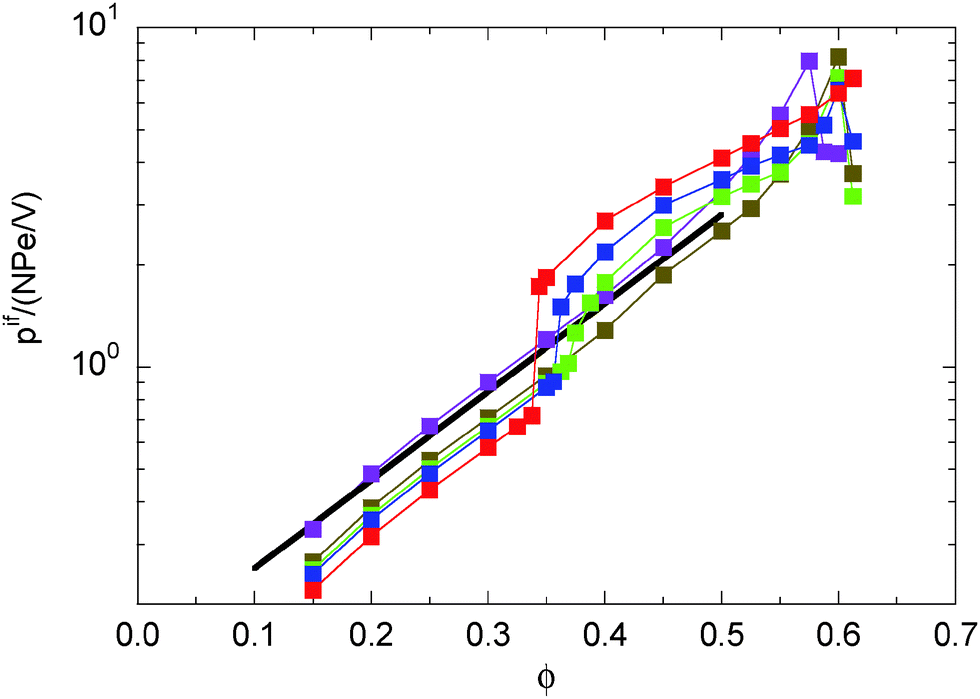

 . The pressure pe at the surface element is