
(De)localization dynamics of molecular excitons: comparison of mixed quantum-classical and fully quantum treatments†
Evgenii
Titov‡
 ,
Tristan
Kopp
,
Joscha
Hoche
,
Alexander
Humeniuk
and
Roland
Mitrić
*
,
Tristan
Kopp
,
Joscha
Hoche
,
Alexander
Humeniuk
and
Roland
Mitrić
*
Institut für Physikalische und Theoretische Chemie, Julius-Maximilians-Universität Wüurzburg, Emil-Fischer-Strasse 42, 97074 Würzburg, Germany. E-mail: roland.mitric@uni-wuerzburg.de
First published on 22nd April 2022
Abstract
Molecular excitons play a central role in processes of solar energy conversion, both natural and artificial. It is therefore no wonder that numerous experimental and theoretical investigations in the last decade, employing state-of-the-art spectroscopic techniques and computational methods, have been driven by the common aim to unravel exciton dynamics in multichromophoric systems. Theoretically, exciton (de)localization and transfer dynamics are most often modelled using either mixed quantum-classical approaches (e.g., trajectory surface hopping) or fully quantum mechanical treatments (either using model diabatic Hamiltonians or direct dynamics). Yet, the terms such as “exciton localization” or “exciton transfer” may bear different meanings in different works depending on the method in use (quantum-classical vs. fully quantum). Here, we relate different views on exciton (de)localization. For this purpose, we perform molecular surface hopping simulations on several tetracene dimers differing by a magnitude of exciton coupling and carry out quantum dynamical as well as surface hopping calculations on a relevant model system. The molecular surface hopping simulations are done using efficient long-range corrected time-dependent density functional tight binding electronic structure method, allowing us to gain insight into different regimes of exciton dynamics in the studied systems.
1 Introduction
Molecular excitons, the electronically excited states of molecular aggregates, underlie many processes of biological and technological importance, such as photosynthesis1 or operation of organic solar cells.2 The development of new, ever more efficient organic electronic devices requires a thorough atomistic understanding of exciton dynamics, including generation of excitons, their delocalization and localization, and excitation energy transfer. On a fundamental level, the molecular exciton dynamics typically must be described by coupled electron-nuclear dynamics involving multiple potential energy surfaces, known as the nonadiabatic dynamics.3The straightforward numerical solution of the full time-dependent Schrödinger equation, allowing one to gain complete insight into the nonadiabatic dynamics, is an intractable task in the case of molecular aggregates due to the large number of electrons and nuclei of which the whole molecular assembly consists. Therefore, more efficient (and approximate) methods and models should be applied to uncover the fate of excitons. The numerical propagation on a grid can be used for model Hamiltonians describing molecular dimers and trimers with a single vibrational degree of freedom (DoF) per monomer.4,5 More degrees of freedom can be treated with multiconfiguration time-dependent Hartree (MCTDH) method.6–8 And for even higher dimensional systems, there are two often used methodologies—(i) mixed quantum-classical approaches, e.g., surface hopping (SH) dynamics,9,10 and (ii) efficient fully quantum treatments, e.g., multiconfigurational Ehrenfest (MCE)11,12 or multi-layer MCTDH (ML-MCTDH).13,14 We also note that the recent classical SQC/MM method (symmetrical quasi-classical windowing model applied to the classical Meyer–Miller vibronic Hamiltonian) developed by Miller and co-workers was shown to accurately describe the exciton dynamics.15,16
The advantages of the surface hopping simulations are relatively low computational cost (especially when combined with fast electronic structure methods) and ability to treat explicitly (though classically) all nuclear DoFs for relatively large molecular systems.17–32 However, in order to account for the quantum nature of nuclei and properly describe decoherence the quantum dynamical treatment is needed.12,14,33–37
To judge the extent of the spatial exciton (de)localization, in the SH simulations the electronic quantities (transition density matrices, molecular orbitals, particle and hole charges, etc.) are analyzed at a certain time at a fixed nuclear configuration, corresponding to a specific point of the SH trajectory.10,30 The subsequent analysis of the whole swarm of trajectories may lead to seemingly very different conclusions about exciton localization/delocalization, depending on the way how this analysis is performed. For example, for a molecular homodimer the ensemble-averaged “fractions of transition density matrices” (FTDMs), representing the fraction of excitation on the left and the right fragments (for precise definition see the Methods, eqn (3)), may stay both equal to 0.5 throughout the simulation, thus implying the exciton delocalization. However, the different analysis of the same ensemble of trajectories, sorting the fragments by the fraction of transition density matrices rather than by geometrically defined criterion (left or right) at each time step, reveals the divergence in FTDM values, with highest fragment accumulating the most of the excitation and the lowest fragment staying almost excitation-free, and thus implies the exciton localization.30 We note that another way of analyzing SH simulations in context of exciton dynamics consists in diabatization based on localization of molecular orbitals on fragments.31,38 And yet another way to model exciton dynamics with SH consists in utilizing an exciton model, which allows for straightforward definition of diabatic states.39,40
In fully quantum simulations based on a diabatic representation, the diabatic electronic state populations are the quantities of choice, which unambiguously show the involvement of each fragment into the exciton wave function. Note that we refer here to locally excited diabatic states (|ge〉 and |eg〉 in the case of a dimer, with g being a ground state of one monomer and e being an excited state of the other monomer). These populations include by definition the integration over nuclear DoFs, thus accounting for all nuclear configurations “covered” by a wave packet. For direct dynamics one may also introduce the operator corresponding to FTDM and use its expectation value to track exciton dynamics.36
In this paper, we relate the two views (quantum-classical and fully quantum) on the exciton (de)localization. To this end, we perform the SH simulations employing the TD-lc-DFTB electonic structure method27,41 on the covalently-linked tetracene dimer42 and analyze the exciton dynamics in this dimer. Subsequently, we show how the dynamics are affected by increasing exciton coupling. To do so, we consider three tetracene dimers differing by a linker between tetracene units. Finally, we perform the quantum dynamical calculations on a model system and demonstrate correspondence between quantum-classical and quantum views on the exciton (de)localization, emphasizing the role of the exciton coupling strength in this process.
2 Methods and models
2.1 Molecular surface hopping calculations
The dynamics of the dimers were modeled employing the TD-lc-DFTB method as implemented in the DFTBaby software package.27,41,43 First, for the dimer from ref. 42 (see Fig. 1), a ground state (GS) molecular dynamics (MD) run was performed at a constant temperature of 300 K to equilibrate the system and sample initial conditions (nuclear positions and velocities) for subsequent surface hopping dynamics.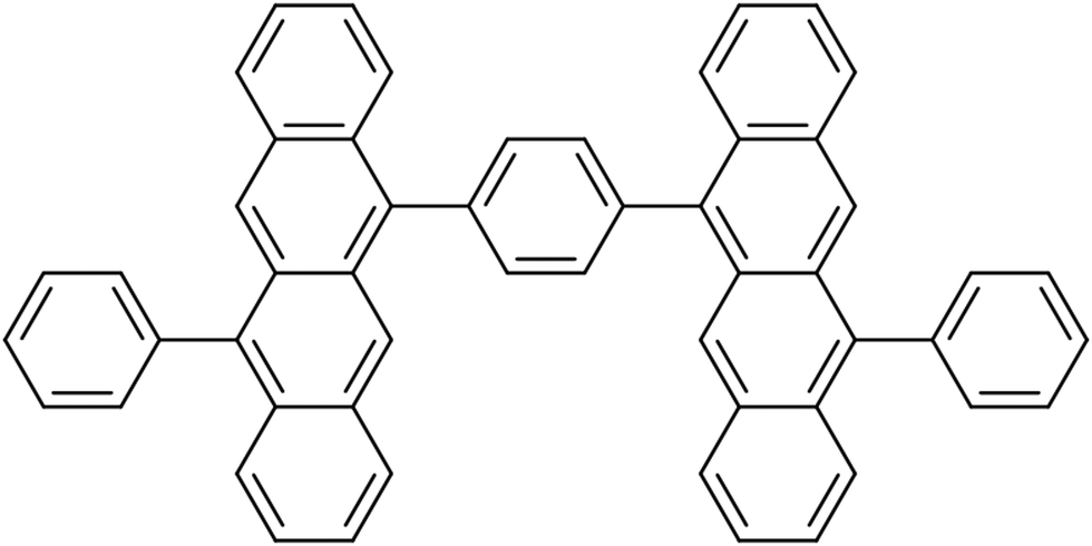 | ||
| Fig. 1 Tetracene dimer from ref. 42. | ||
The Berendsen thermostat44 was used to control the temperature. The optimized ωB97X-D45/6-31G*46 geometry and randomly generated velocities (corresponding to 300 K) were used to initialize the GS MD run. The geometry optimization was done using Gaussian 16.47 The time step for the GS MD was set to 0.2 fs. Initial conditions for surface hopping dynamics were sampled every 100 fs starting after 2 ps. In total, 100 initial conditions were sampled.
For the calculation of excited states we used a reduced active space composed of the highest 30 occupied and the lowest 30 virtual orbitals, denoted as 30 × 30 in what follows. This space provides good compromise between accuracy of excitation energies and the computational time needed for surface hopping calculations. Excitation energies and corresponding oscillator strengths were computed for selected geometries in order to simulate thermally broadened absorption spectrum. For all the sampled nuclear configurations the S0 → S1 transition was found to be the most intense one. Therefore, all surface-hopping trajectories were launched from the S1 state. The nonadiabatic dynamics were simulated employing Tully's surface hopping approach9 with modified calculation of hopping probabilities48 using local diabatization scheme to propagate the electronic wave function.49,50 The standard energy-based decoherence correction was applied.51 The time step for surface hopping dynamics was set to 0.1 fs. Each trajectory was propagated up to 100 fs. The ground and two lowest singlet excited states were included in surface hopping simulations.
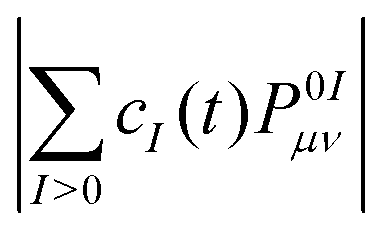
The adiabatic populations were computed using two methods, which we name “surfaces” and “wavevector” following ref. 52. In the “surfaces” method, the adiabatic populations are computed as fractions of trajectories in a given state, whereas in the “wavevector” method they are given by squared absolute values |cI(t)|2 of time-dependent coefficients of the electronic wave function (Φel(t) = ΣIcI(t)ΦI, ΦI are the adiabatic electronic wave functions) averaged over the swarm of trajectories.
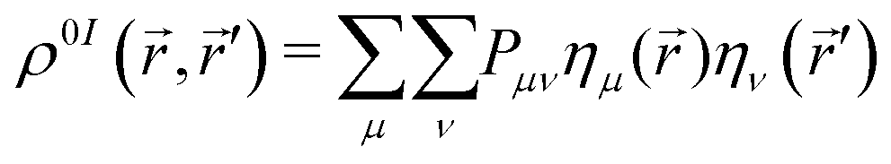
The exciton dynamics were analyzed using the reduced first-order spinless transition density matrix ρ0I(![[r with combining right harpoon above (vector)]](https://www.rsc.org/images/entities/i_char_0072_20d1.gif) , ′) between ground (0) and excited (I) electronic states which in the atomic orbital basis {ημ()} reads:
, ′) between ground (0) and excited (I) electronic states which in the atomic orbital basis {ημ()} reads:
 | (1) |
 | (2) |
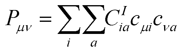
The Pμν elements were used further to calculate “fraction of transition density matrix” FTDMXY showing the partitioning of excitation between two tetracene fragments:
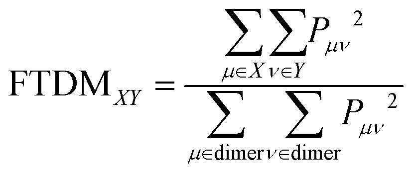 | (3) |
 (note that the ground-state coefficient is not used). This is the “wavevector” method for calculating FTDM.
Further, as mentioned in the introduction, averaging FTDMLL(RR)(t) over the swarm of trajectories masks information about exciton (de)localization for individual trajectories. Therefore, we also define highest (![[script letter H]](https://www.rsc.org/images/entities/char_e142.gif) ) and lowest (
) and lowest (![[script L]](https://www.rsc.org/images/entities/char_e144.gif) ) monomers (fragments) as follows. At each time step, for each trajectory we determine the fragment with the highest FTDM value (and hence automatically the other one, with the lowest FTDM value), FTDM(t) > FTDM(t) (note that FTDM and FTDM are diagonal elements of the FTDM matrix). After that we calculate the average of FTDM and FTDM over the whole ensemble of trajectories.
) monomers (fragments) as follows. At each time step, for each trajectory we determine the fragment with the highest FTDM value (and hence automatically the other one, with the lowest FTDM value), FTDM(t) > FTDM(t) (note that FTDM and FTDM are diagonal elements of the FTDM matrix). After that we calculate the average of FTDM and FTDM over the whole ensemble of trajectories.
In addition, we calculate a participation number (PN) (which is also known as inverse participation ratio (IPR)) using two recipes, PN1 = (FTDMLL2 + FTDMRR2)−1![[thin space (1/6-em)]](https://www.rsc.org/images/entities/char_2009.gif) 53 and
53 and 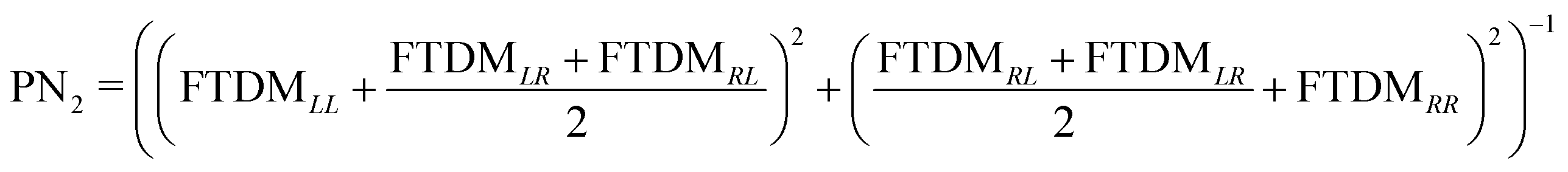 .54 This quantity reflects the extent of exciton (de)localization over the fragments composing a molecule. In the case of complete delocalization over two monomers (FTDMXX ≈ 0.5 ∀ X) PN ≈ 2, while localization on a single fragment (FTDMX1X1 ≈ 1, FTDMX2X2 ≈ 0) corresponds to PN ≈ 1. PN1 accounts for local excitations only, whereas PN2 takes into account the charge-transfer elements of the FTDM matrix as well.
Furthermore, we calculate the fraction of trajectories, having FTDMXX in a certain interval 0.0 + 0.1j < FTDMXX ≤ 0.1 + 0.1j (j= 0,1,2,…,9) at a given time t. Constructing a relative frequency distribution from such fractions allows one to visualize the extent of spatial (de)localization of the exciton at a fixed time. Specifically, large peaks at small and big values of FTDMXX correspond to localization of the exciton, whereas peaks in the middle reflect delocalization. Another characteristic, which we introduce, is the fraction of trajectories, possessing an FTDM gap, defined for fragment X as FTDMgap = maxt(FTDMXX) − mint(FTDMXX) for each trajectory separately, in a certain interval 0.0 + 0.1j < FTDMgap ≤ 0.1 + 0.1j (j = 0,1,2,…,9). Large values of this gap indicate that during a nonadiabatic molecular dynamics run, FTDMXX, reflecting localization on a given monomer X, experiences substantial changes, i.e., the excitation “travels away” or, oppositely, “visits” the fragment of interest.
2.2 Two-state two-dimensional model; quantum dynamics and surface hopping for the model system
We consider a dimeric exciton model with one vibrational degree of freedom per monomer (Qi, i = 1, 2) and constant coupling v.4,55 The diabatic Hamiltonian matrix reads: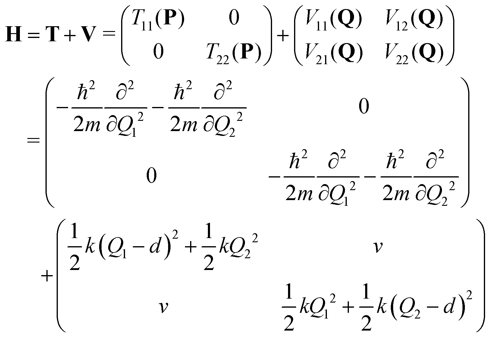 | (4) |
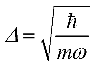
 .56 Here, d is the displacement of the excited-state PES with respect to the ground-state PES, and m is the mass, taken to be the reduced mass of the 62nd normal mode of the tetracene monomer (reported in the output of Gaussian 16 frequency calculation for the excited state). The displacement d, needed to construct the Hamiltonian, is thus obtained as
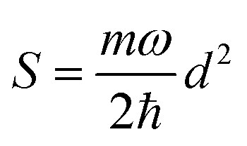
  . The force constant is given by k = mω2. Thus, we obtain S = 0.53, d = 0.096 a.u., m = 17412 a.u. (9.55 amu), ω = 0.00671 a.u. (1473 cm−1). The exciton coupling v can be determined as minus half of the exciton splitting.
Quantum dynamical calculations were done on a grid using the second order differences (SODs) method with Fourier transform:57
 | (5) |
Surface hopping calculations were carried out in the adiabatic representation. Newton's equations of nuclear motion were integrated using the velocity Verlet algorithm with a time step of 0.05 fs. The electronic Schrödinger equation was integrated using the Runge–Kutta method of fourth order with 2000 steps per nuclear time step. Initial conditions (100 {Qi (t = 0), Pi (t = 0)} pairs in total) were sampled from the Wigner function of the vibrational ground state (of the electronic ground state) in the harmonic approximation. The calculations were performed without and with the energy-based decoherence correction.51 The diabatic populations, in turn, were obtained either expressing the wave function of the current adiabatic state in the diabatic basis (“surfaces” method) or converting full electronic wave function to the diabatic basis (“wavevector” method), and then averaging over the swarm of trajectories. Using diabatic probabilities, we also define the highest fragment, in analogy with FTDM. Furthermore, we calculated the diabatic populations using a “mixed” approach based on a nuclear-electronic density matrix.52 The mathematical details are presented in SI6 (ESI†).
3 Results and discussion
3.1 Tetracene dimer with a weak exciton coupling
First, we have investigated the performance of different electronic structure methods for low-lying excited states of the tetracene dimer from ref. 42 and assessed TD-lc-DFTB results (see SI1, ESI†). Whereas the TD-lc-DFTB excited states are blue-shifted in comparison to more accurate methods, the nature of the two lowest excited states (S1 and S2) is well reproduced by TD-lc-DFTB. The S1–S2 exciton splitting is ∼0.13 eV at the TD-lc-DFTB (30 × 30) level of theory and ∼0.05 eV when using higher-level methods.Next, we have performed the ground-state Born–Oppenheimer molecular dynamics at constant temperature, in order to prepare initial conditions for subsequent surface hopping dynamics and also reveal the effect of conformational disorder on exciton states. The latter are delocalized over both tetracene units for the ground-state minimum geometry as can be seen from the corresponding natural transition orbitals58 (Fig. S2, ESI†). Further, for the snapshots, selected from the GS MD trajectory, the vertical absorption spectra were computed with TD-lc-DFTB (30 × 30), requesting four lowest excited states. For all geometries, the S0 → S1 transition was found to be much more intense than the S0 → S2 transition. S3 and S4 states are separated by a sizable gap from the S2 state what allows us to include only S0, S1, and S2 states into surface hopping simulations, and neglect higher lying excited states. For details see Fig. S3 (ESI†).
We have then launched the surface hopping trajectories from the S1 state. The electronic state populations, calculated using the “sufaces” and “wavevector” methods, are presented in Fig. 2. Similarly to what we found for the tetracene trimer dynamics,30 the tetracene dimer remains mostly in the S1 state (population of >0.9), while the S2 state is only slightly populated (population of <0.1), throughout 100 fs of simulation. We do not observe a return to the ground state within this time period. We note that 85% of all the trajectories evolved without making any hops within 100 fs. For these trajectories the dynamics are thus adiabatic (occurring on the S1 potential energy surface). The populations calculated with the “surfaces” method are similar to those obtained with the “wavevector” method.
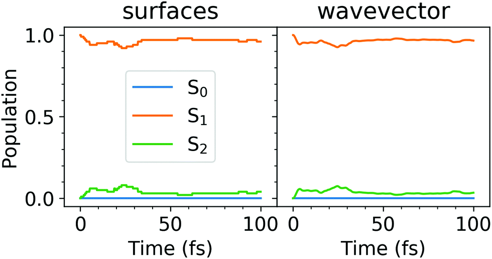 | ||
| Fig. 2 Electonic state populations, calculated using the “surfaces” (left) and “wavevector” (right) methods. | ||
The evolution of adiabatic state populations shown in Fig. 2 does not reveal however the exciton dynamics in the dimer. In order to disclose the dynamic exciton localization/delocalization, arising due to the nuclear motion, we analyze transition density matrices along the surface hopping trajectories. Specifically, we compute the FTDM descriptor (see eqn (3)) for the current electronic state and the electronic wavevector as a function of time. The ensemble-averaged FTDM values for the L and R fragments are shown in Fig. 3 (upper panels).
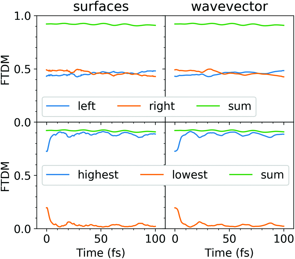 | ||
| Fig. 3 Ensemble-averaged FTDMLL(RR)(t) (upper panels) and FTDM()(t) (lower panels), calculated using the “surfaces” (left) and “wavevector” (right) methods. The sums FTDMLL(t) + FTDMRR(t) (upper panels) and FTDM(t) + FTDM(t) (lower panels) are also shown. | ||
Both, FTDMLL and FTDMRR, remain close to 0.5 throughout the simulation. Thus, on average, one finds delocalizaion of the exciton over two fragments. We note also that the sum of FTDMLL and FTDMRR is close to 1, indicating that charge-transfer elements (FTDMXY with X ≠ Y) as well as FTDM values for the other fragments (e.g., benzene rings) are small. However, this averaged picture hides what happens on a single trajectory level. Therefore, we analyze FTDM()(t) (Fig. 3 (lower panels)).
Firstly, we note that the FTDM values at the beginning, at t = 0 fs, are very different for the highest and the lowest fragments, namely FTDM ≈ 0.75 and FTDM ≈ 0.2. This shows the effect of the ground-state MD on the nature of excitonic states. Namely, structural distortions caused by ground-state MD lead to differences between monomer geometries (what may be termed conformational disorder) and, hence, induce partial exciton localization on one of two fragments. This initial partial localization is also seen in the distribution of trajectories over FTDM values for geometrically defined fragments (Fig. 4 (left column)), which shows larger values closer to 0 and 1 rather than to 0.5.
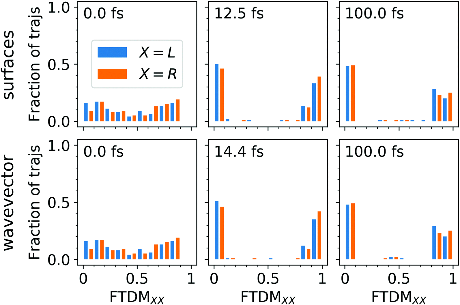 | ||
| Fig. 4 Fraction of trajectories, having a certain FTDMXX value: 0.0 + 0.1j < FTDMXX ≤ 0.1 + 0.1j (j = 0, 1, 2,…,9), for 0 fs (left column), first local maximum of FTDM (middle column), and 100 fs (right column). The upper row for the “surfaces” FTDM, and the lower row for the “wavevector” FTDM. | ||
Secondly, FTDM rises very rapidly and reaches the maximum value at 12.5 fs (“surfaces” method) or 14.4 fs (“wavevector” method). These times are close to ∼17 fs found for the tetracene trimer.30 This rise corresponds to the further exciton localization (at the single trajectory level), induced by nuclear dynamics in excited states. At the maxima, distributions of trajectories over FTDM values become very peaked at low and high values of FTDM (Fig. 4 (middle column)). The localization is preserved till the end of the simulation (see Fig. 3 (lower panels) and distributions for t = 100 fs in Fig. 4 (right column)). Notably, FTDM(t) and FTDM(t) exhibit perceptible oscillations, which correlate with CC bond vibrations (Fig. S4, ESI†). The exciton localization and the oscillations are also clearly seen in the time-evolution of the participation number (Fig. S5, ESI†).
Further, once localized, the exciton may either stay trapped on a particular monomer (within 100 fs) or be transferred between the monomers. This can be seen from the relative frequency distribution of trajectories over FTDM gap (Fig. S6, ESI†), as well as the FTDMLL and FTDMRR time evolutions for single trajectories (Fig. S7, ESI†).
Finally, we note that the “surfaces” FTDM curves are very similar to the “wavevector” FTDM curves (see Fig. 3).
3.2 Tetracene dimers with a stronger exciton coupling
In order to investigate the influence of the exciton coupling strength on the exciton localization dynamics, we now introduce different linkers connecting the tetracene units. Different linkers result in different exciton couplings of monomers, which is reflected in different exciton splittings. In particular, we have considered (i) phenyl linker (weak exciton coupling), (ii) –C![[triple bond, length as m-dash]](https://www.rsc.org/images/entities/char_e002.gif) C– linker (intermediate exciton coupling), and (iii) –C
C– linker (intermediate exciton coupling), and (iii) –C![[double bond, length as m-dash]](https://www.rsc.org/images/entities/char_e001.gif) C– linker (strong exciton coupling), as shown in Fig. 5. The corresponding exciton splittings calculated with TD-lc-DFTB (using an active space of 40 occupied and 40 virtual orbitals) are (i) 0.13 eV, (ii) 0.49 eV, and (iii) 0.69 eV, respectively (Fig. 5).
C– linker (strong exciton coupling), as shown in Fig. 5. The corresponding exciton splittings calculated with TD-lc-DFTB (using an active space of 40 occupied and 40 virtual orbitals) are (i) 0.13 eV, (ii) 0.49 eV, and (iii) 0.69 eV, respectively (Fig. 5).
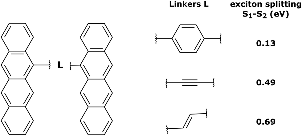 | ||
| Fig. 5 Tetracene dimers with different linkers considered in this work, and the corresponding exciton splittings calculated with TD-lc-DFTB. | ||
To demonstrate the effect of coupling, we have performed ten nonadiabatic dynamics runs for each of the dimers, starting always from a ground-state minimum geometry but with random velocities (corresponding to a temperature of 300 K). The time evolution of FTDMXX for single trajectories of the three tetracene dimers is shown in Fig. 6a and b. It is seen that the weak exciton coupling favours localization, while for the stronger couplings the exciton is more delocalized. This situation is also clearly seen in the histograms of time steps with respect to the FTDMXX values (Fig. 6c and d). The shown histograms are averages over ten trajectories.
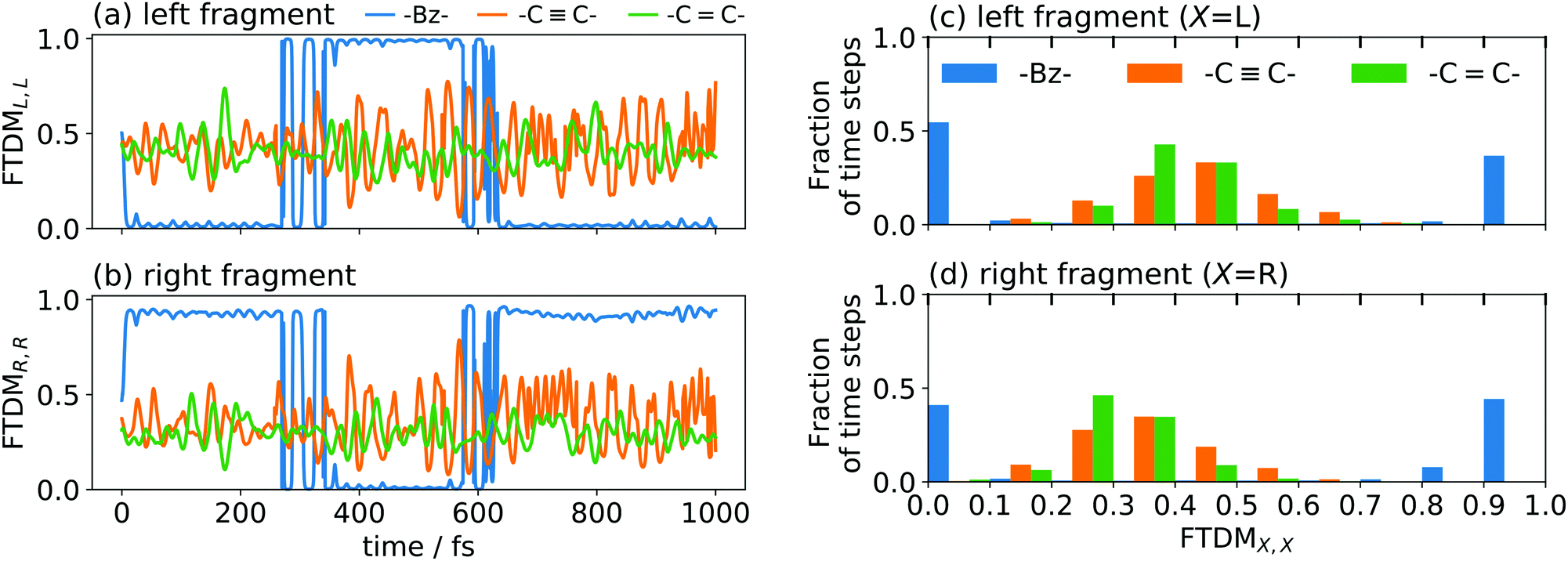 | ||
| Fig. 6 (a and b) FTDMXX as a function of time for three tetracene dimers differing by a linker, for single trajectories, for left (a) and right (b) fragments. (c and d) Distributions of time steps over FTDM values for left (c) and right (d) fragments (histograms are averaged over ten trajectories). | ||
3.3 Quantum dynamics and surface hopping for the two-state two-dimensional model
As we have seen in Fig. 3, the interpretation of surface hopping results regarding exciton localization/delocalization depends on what exactly is averaged, FTDMLL (FTDMRR) or FTDM (FTDM). A question arises: How do these findings relate to fully quantum mechanical treatment of a molecule? In order to answer this question, we consider the dimeric exciton model (4).
The exciton coupling v can be determined as minus half of the exciton splitting. We note that the transition dipole moment of the S1 state of a tetracene monomer is directed along the short molecular axis,59 and, hence, the tetracene dimers studied here are examples of J-aggregates. For the latter, the coupling is negative.60 Using the smallest (0.13 eV) and the largest (0.69 eV) exciton splittings of Fig. 5, we obtain v = −0.065 eV (≈−0.002 a.u.) and v = −0.345 eV (≈−0.013 a.u.), for weak and strong couplings, respectively. We also note that for the tetracene dimer of Fig. 1 the exciton splitting is 0.13 eV at the TD-lc-DFTB (30 × 30) level, used for the SH dynamics described in Section 3.1.
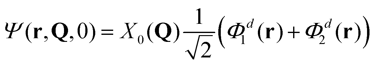
The total molecular wave function may be written either in the diabatic representation or in the adiabatic one. The adiabatic electronic states are obtained from the diabatic states by means of the diabatic-to-adiabatic transformation (DAT) (mathematical details are given in SI5, ESI†). As in the case of surface hopping simulations we initiate the dynamics from the adiabatic S1 state, since this state is bright, whereas the S2 state is dark (see Table S1 of the ESI†). Further, we chose the initial nuclear wave function to be the vibrational ground-state wave function of the electronic ground state (S0), i.e., the initial total wave function reads:
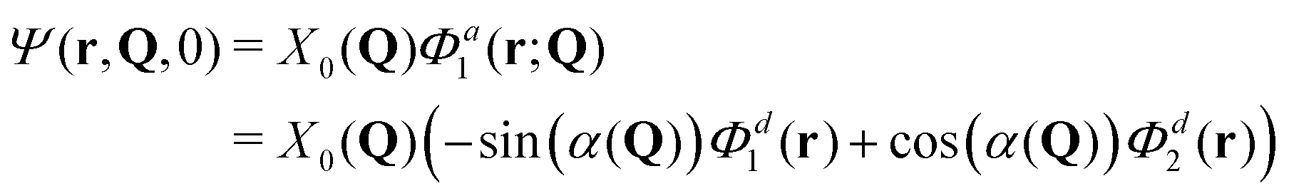 | (6) |
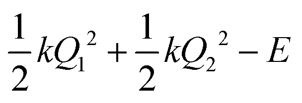 , centered at (Q1, Q2) = (0, 0) (E is a relatively large energy offset). The initial nuclear wave function is therefore given by:
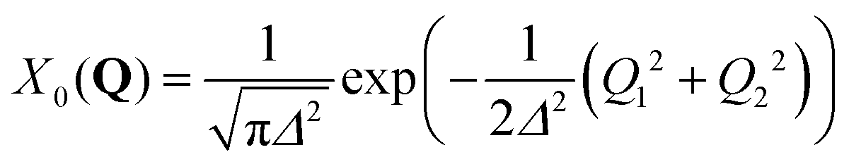 | (7) |
 .
.
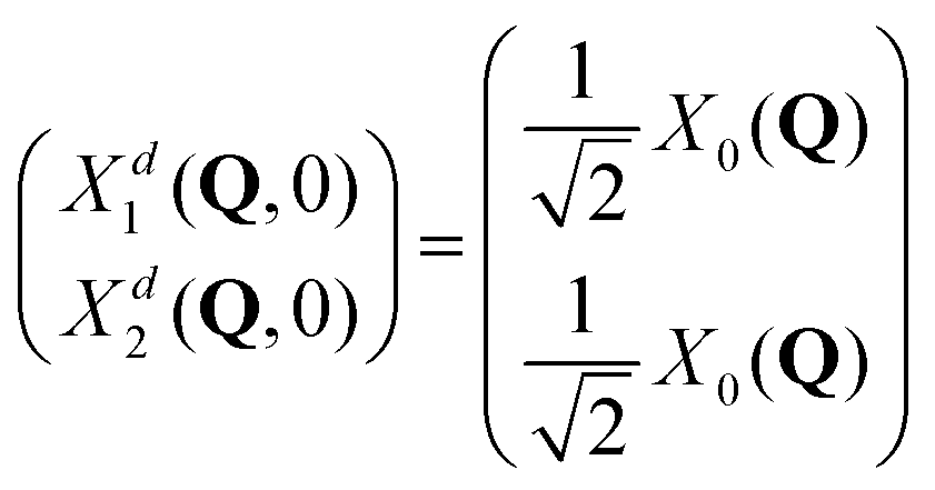
The initial wave packets in the diabatic picture are then (see SI5, ESI†):
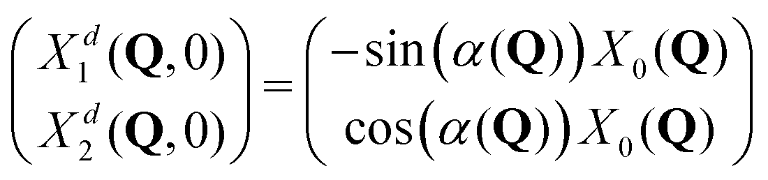 | (8) |
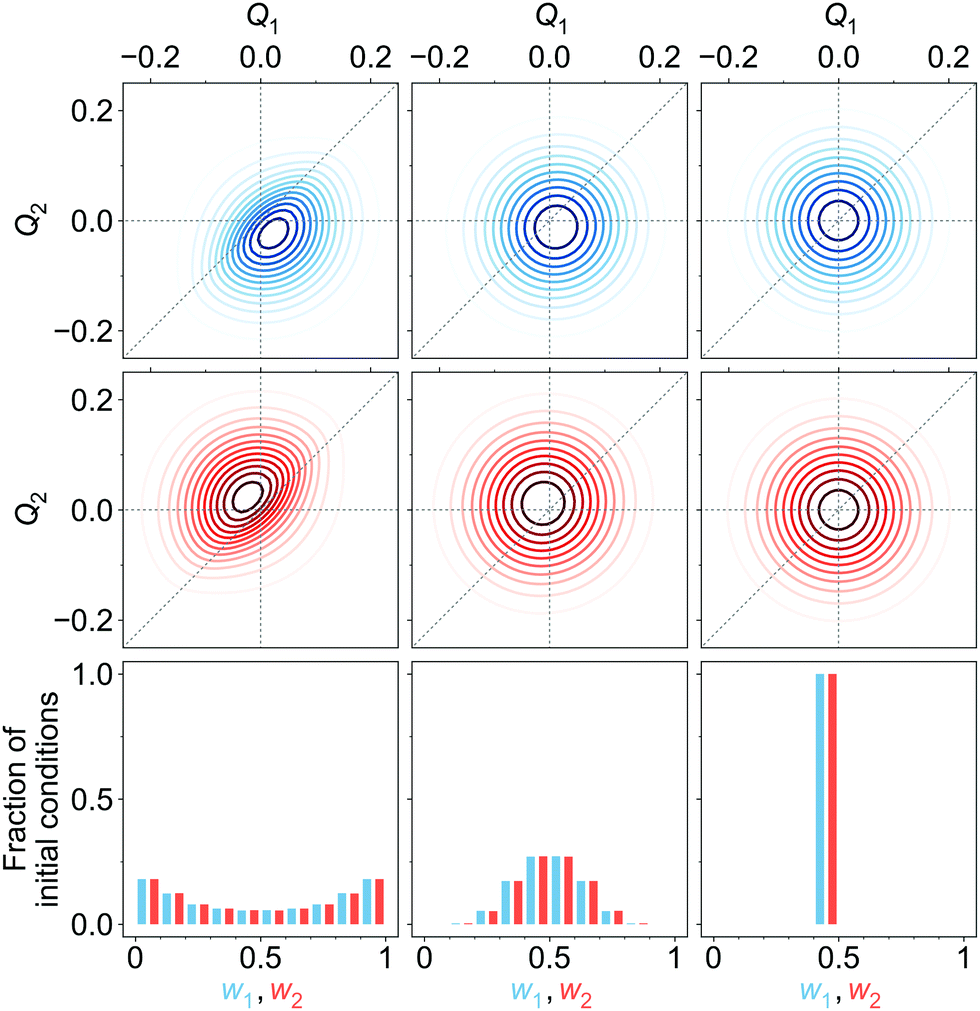 | ||
| Fig. 7 Upper and middle rows: Initial diabatic wave packets (at t = 0) for [adiabatic initial condition (6) and weak coupling (v = −0.065 eV)] (left column), [adiabatic initial condition (6) and strong coupling (v = −0.345 eV)] (middle column), and [diabatic initial condition (9) (irrespective of the coupling)] (right column). Xd1(Q, 0) is shown in blue (upper row), Xd2(Q, 0) is shown in red (middle row). Lower row: Distribution of one million initial conditions (geometries) with respect to the w1 (bluish) and w2 (reddish) coefficients (see eqn (12)) for respective diabatic wave packets shown in the first two rows. | ||
Another choice of initial conditions that is often made to study ultrafast quantum dynamics7,14,62 is:
 | (9) |
 | (10) |
At this point, we can already anticipate a relation of quantum mechanical treatment to the surface hopping approach in the context of exciton (de)localization. Let us imagine a single trajectory Q(t), which is a typical outcome of surface hopping simulations. At time t = t′, the nuclear configuration is described by Q = Q′. Substituting t′ and Q′ in the expression for the total wave function (eqn (S1) in the ESI†) we obtain:
 | (11) |
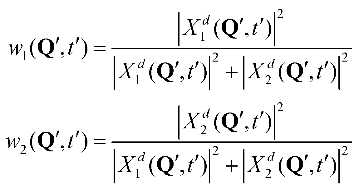 | (12) |
In surface hopping simulations, one runs a swarm of trajectories, thus having many geometries for a given time t′. For all these geometries, one can calculate w1, w2 coefficients and then analyze distribution of trajectories over these coefficients, at t = t′. We do this now for t = 0. In order to prepare initial conditions (initial geometries), we sample one million points {Q′} from the squared initial nuclear wave function X02(Q). Then we calculate w1, w2 coefficients (12) for these sampled geometries using diabatic wave packets of Fig. 7 and construct relative frequency distibutions of initial conditions (geometries) over the w1, w2 coefficients. These distributions are shown in the lower row of Fig. 7.
For [adiabatic initial condition (6) and weak coupling (v = −0.065 eV)], the largest fraction of initial geometries is characterized by w1 ≈ 1, w2 ≈ 0 and w1 ≈ 0, w2 ≈ 1 (left lower corner of Fig. 7). The distribution is remarkably similar to that of Fig. 4a, obtained from surface hopping calculations on the weakly coupled tetracene dimer. The observed situation corresponds to (partial) exciton localization on a single-geometry level. On the contrary, for [adiabatic initial condition (6) and strong coupling (v = −0.345 eV)], the distribution is dominated by w1 ≈ w2 ≈ 0.5 (middle of the lower row of Fig. 7), and thus corresponds to the exciton delocalization. Lastly, for [diabatic initial condition (9) (irrespective of the coupling)], w1 = w2 = 0.5 for any initial geometry (right lower corner of Fig. 7), since Xd1(Q, 0) = Xd2(Q, 0) (see (10) and (12)).
Further, looking at Fig. 7 we see that the overlap of diabatic nuclear wave packets is different for different initial conditions: it increases from the left to the right. The single-geometry delocalization also increases from the left to the right of Fig. 7 (see the last row). Indeed, if by time t = t′ the overlap of nuclear wave packet moduli becomes small, then for most of geometries {Q′} only one of the Xd1(Q′, t′) and Xd2(Q′, t′) coefficients in (11) will be relatively large, whereas the other one will be close to zero. Thus, the effective electronic wave function will be either ∼Φd1(r) or ∼Φd2(r). In other words, the exciton gets localized on one of two monomers, from this point of view. On the contrary, if 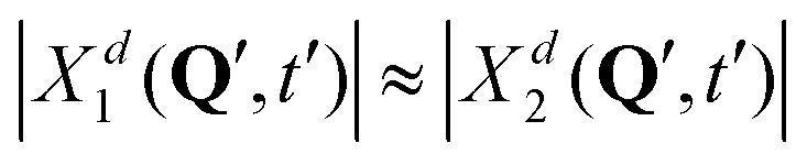 for most of {Q′}, the exciton is delocalized over two monomers. Thus, the overlap of diabatic nuclear wave packet moduli can be introduced as a measure reflecting the trajectory-based view on exciton (de)localization in fully quantum mechanical calculations:
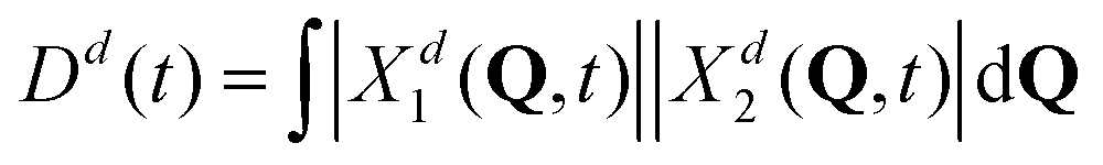 | (13) |
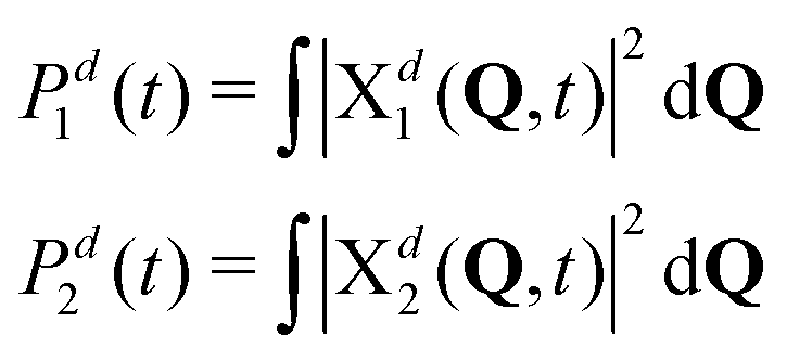
Naturally, in quantum dynamics, the diabatic state populations are the proper quantities to monitor exciton (de)localization from quantum mechanical point of view. These populations are defined as:
 | (14) |
 | (15) |
We have performed quantum dynamics calculations for initial conditions of Fig. 7. Namely, we have considered four cases: (i) [adiabatic initial condition (6) and weak coupling (v = −0.065 eV)], (ii) [adiabatic initial condition (6) and strong coupling (v = −0.345 eV)], (iii) [diabatic initial condition (9) and weak coupling (v = −0.065 eV)], and (iv) [diabatic initial condition (9) and strong coupling (v = −0.345 eV)].
The adiabatic and diabatic populations of adiabatic state 1 and diabatic state 1, respectively, are shown in Fig. 8a. The diabatic populations are computed according to (14), and they are readily available since the propagation is done in the diabatic representation. We emphasize that the diabatic states Φd1(r) and Φd2(r) are locally excited states and therefore their populations directly show extent of the exciton (de)localization. The adiabatic populations are computed using the same formulae (14), but with superscript d replaced with a, i.e. using adiabatic nuclear wave packets. The latter are obtained from the diabatic ones using the DAT matrix (see SI5, ESI†).
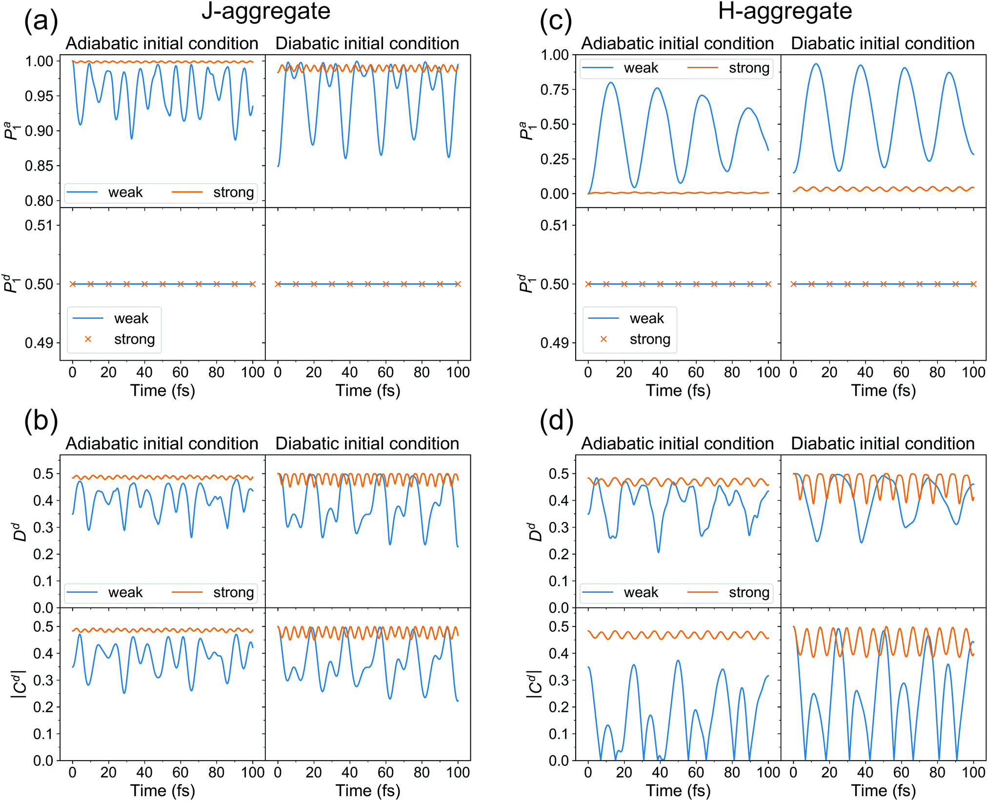 | ||
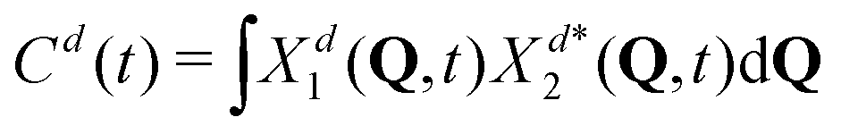
| Fig. 8 Quantum dynamics results for J- (a and b) and H- (c and d) aggregate. (a and c) Adiabatic Pa1(t) (upper row) and diabatic Pd1(t) (lower row) populations of adiabatic state 1 and diabatic state 1, respectively, for adiabatic (left column) and diabatic (right column) initial conditions, for weak (blue) and strong (orange) couplings. (b and d) (De)localization (upper row) and coherence |Cd(t)| (lower row) measures for adiabatic (left column) and diabatic (right column) initial conditions, for weak (blue) and strong (orange) couplings. | ||
First of all, we see that the adiabatic populations at t = 0 are exactly 1 for initial conditions (i) and (ii), and less than 1 for initial conditions (iii) and (iv). Therefore, initial conditions (i) and (ii) correspond better to the initial conditions used in the surface hopping simulations, as already pointed out above. Further, the Pa1 population for (i) resembles the population dynamics observed in surface hopping simulations (Fig. 2). Namely, there is an ultrafast S1 → S2 (Φa1 → Φa2) population transfer resulting in S1 (Φa1) population decrease from 1 to ∼0.9. For weak coupling the population transfer between adiabatic states is stronger than for the strong coupling. It is expected since a larger coupling leads to a larger exciton splitting and thus a reduced probability of nonadiabatic transitions between S1 and S2. Remarkably, for all considered initial conditions (i–iv), the diabatic populations are always equal to 0.5 throughout the propagation. This means that the delocalized exciton remains delocalized, from fully quantum mechanical point of view. This delocalization should be viewed as a “statistical” delocalization with respect to the electronic subsystem (note that the total nuclear-electronic system is in a pure state). The diabatic populations Pd1(2) bear the same meaning as FTDMLL(RR) curves in Fig. 3 (upper panels).
Fig. 8b shows the time evolution of (de)localization and coherence measures for cases (i–iv). First of all, looking at Dd(t) for adiabatic initial condition we see that at t = 0 the exciton is more localized (from trajectory-based view) for weak coupling than for the strong coupling (Dd(0) value is smaller for the weak coupling). We have already come to this conclusion inspecting distributions of Fig. 7. For diabatic initial condition, the exciton is delocalized irrespective of the coupling, since the initial diabatic wave packets are the same. Next, we see that the (de)localization measure is not constant during dynamics, but shows delocalized-localized interconversions with time. This is in contrast to the diabatic populations of Fig. 8a.
Thus, while delocalization is established from fully quantum point of view, the trajectory-based localization may still be observed, simultaneously with the quantum delocalization. This finding is very similar to the surface hopping results of Fig. 3. We note, however, that in surface hopping simulations, once localized, the exciton remains mostly localized, while in our quantum dynamical calculations we observe a “periodic” behaviour, i.e. the exciton experiences multiple delocalization–localization transitions. It is most probably because of low dimensionality of our quantum dynamical model, allowing nuclear wave packets to revisit the same region of configurational space multiple times. It is also seen that the extent of dynamic localization is much larger for the weak coupling than for the strong coupling. For the latter, the exciton remains essentially delocalized.
The absolute value of coherence shows very similar behaviour to that of Dd(t). We also note that Dd(t) and |Cd(t)| must be smaller or equal to 0.5 at any time (this can be shown using the Cauchy–Bunyakovsky–Schwarz inequality and noting that Pd1(t)Pd2(t) ≤ 0.25 ∀ t). The 0.5 values correspond to complete delocalization and maximal coherence, respectively.
It is also interesting to see how these measures behave for an H-aggregate. In this case the coupling v is positive and the transition to the upper adiabatic surface is allowed. The adiabatic initial condition is thus:
 | (16) |
Diabatic wave packets at selected times corresponding to local minima and maxima of Dd(t) are shown in Fig. 9a for the J-aggregate and Fig. 9b for the H-aggregate. Comparing to Fig. 8b and d, one can see that localization corresponds to spatial separation of wave packets (more precisely, their moduli). Interestingly, coherence may become zero for rather large Dd values. It comes from the fact that the integrand (its real and imaginary parts) in (15) may be positive in one part of Q-space and negative in the other one, what may result in zero coherence.
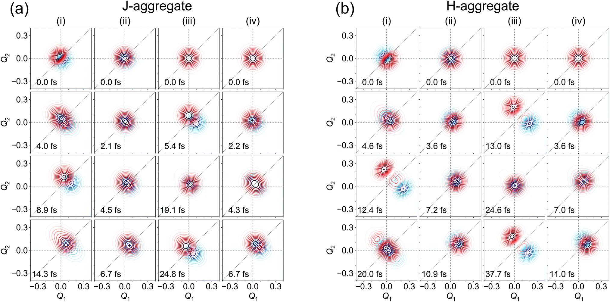 | ||
| Fig. 9 Moduli of diabatic wave packets at selected times for J- (a) and H- (b) aggregates, for (i) [adiabatic initial condition (6) and weak coupling] (left column), (ii) [adiabatic initial condition (6) and strong coupling] (second left column), (iii) [diabatic initial condition (9) and weak coupling] (second right column), and (iv) [diabatic initial condition (9) and strong coupling] (right column). |Xd1(Q, t)| is shown in blue, |Xd2(Q, t)| is shown in red. | ||
To enable a direct comparison of quantum dynamics results with mixed quantum-classical results, we performed SH calculations on the model system defined by (4). The SH results are shown in Fig. 10. The magnitude of the adiabatic population transfer calculated using the “surfaces” method agrees qualitatively with quantum dynamical results (cf.Fig. 8a and c). However, the SH fails to reproduce quantum beatings observed in quantum dynamical adiabatic populations, in agreement with a recent report on exciton dynamics in a heterodimer.63 The adiabatic populations calculated using the “wavevector” method deviate considerably from the “surfaces” populations for the weakly coupled J-aggregate (the top left plot in Fig. 10). The use of decoherence correction expectedly improves the agreement (compare with Fig. S9 (ESI†), where results without decoherence correction are presented), but the difference is still large. This disagreement stems from frustrated hops to the upper adiabatic surface.
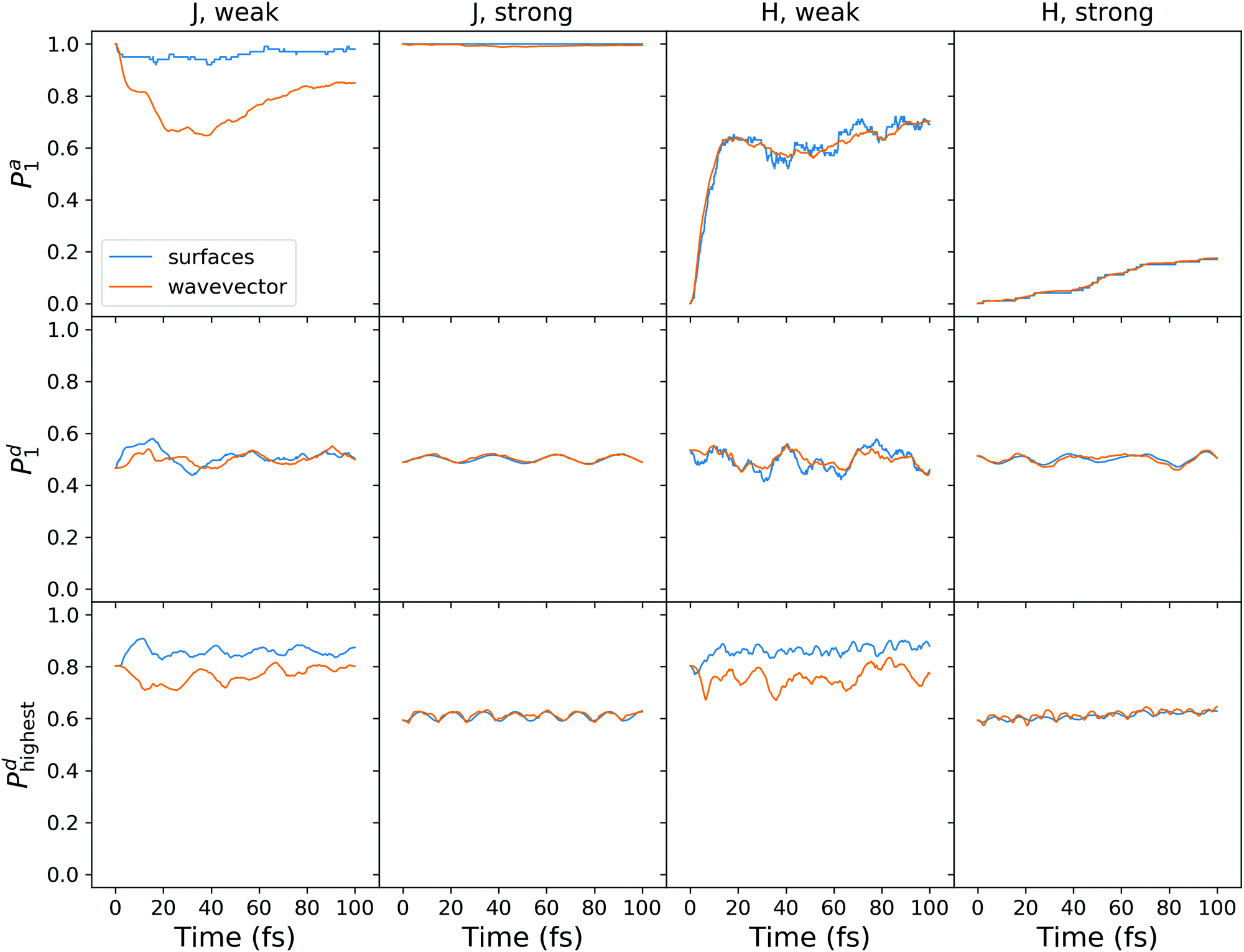 | ||
| Fig. 10 Surface hopping calculations with decoherence correction for the model system (4). Shown are the results for the J- and H-aggregates with weak and strong diabatic coupling. | ||
The diabatic populations fluctuate around 0.5, in agreement with the quantum dynamical results (Fig. 8a and c), and with the FTDMLL(RR) curves in Fig. 3 (upper panels). Importantly, the diabatic population of the highest fragment Pd clearly demonstrates the difference in trajectory-based exciton localization between the weak and the strong coupling cases. Pd values near 0.8 found for the weak coupling case correspond to the more localized excitons, whereas values of ∼0.6 observed for the strong coupling reveal more delocalized excitons.
We also observe a distinct difference between the “surfaces” and the “wavevector” methods for Pd in the case of the weak coupling. At short times, while “surfaces” Pd increases (corresponding to more localization), “wavevector” Pd decreases (corresponding to more delocalization). We also note that the use of the decoherence correction does not affect this behaviour (Fig. S9, ESI†). Interestingly, this difference is not observed in the FTDM curves of Fig. 3 (lower panels), for the multidimensional molecular system. For the model system, the rise of delocalization at short times can be inferred from Dd curves in Fig. 8b and d (for the weak coupling and adiabatic initial condition). In addition, we have tested the “mixed” method of ref. 52 for calculation of diabatic populations. The comparison of the “surfaces”, “wavevector”, and “mixed” methods is presented in Fig. S10 and S11 (ESI†). For the weak diabatic coupling, the “mixed” diabatic populations are closer to the “surfaces” populations, whereas for the strong diabatic coupling the “mixed” populations agree better with the “wavevector” populations.
We must stress that we have considered here only the exciton dynamics in a closed system, while leaving open systems64–69 apart. The interaction with environment accounted for in the open system dynamics may lead to ultimate exciton localization, from the fully quantum point of view.66 In this respect, we note that the lowest vibronic state of the weekly coupled J-aggregate is a delocalized state (Pd1 = Pd2 = 0.5) with coherence Cd ≈ 0.4 (see SI7, ESI†).
Finally, we considered the case of an initially localized excitation, corresponding to the initial total wave function Ψ(r, Q, 0) = X0(Q)Φd1(r), for the weakly coupled J-aggregate. The results are shown in SI8 (ESI†). In this case, the evolution of exciton (de)localization is clearly identified from the diabatic population dynamics (Pd1(t)), whereas large Pd(t) values and the Dd(t) behaviour confirm the single-geometry-localization inherent to the weak coupling.
4 Conclusions
We have addressed the issue of molecular exciton (de)localization on the example of molecular homodimers. Our main goal was to explain what should be understood as “exciton localization” and “exciton delocalization” in mixed quantum-classical dynamics simulations (surface hopping in our case) and how these phenomena relate to fully quantum dynamical treatment of the dimer. In mixed quantum-classical trajectory-based simulations, lacking nuclear wave functions per se, nuclear configuration (molecular structure) at any given time, for any given trajectory is defined by a set of nuclear coordinates, without any uncertainty. For this molecular structure, the exciton localization may be readily analyzed using, e.g., fraction of transition density matrix (FTDM) or natural transition orbitals (NTOs). For perfectly symmetric geometry of the molecular dimer, the exciton is delocalized irrespective of exciton coupling between monomers forming the dimer. Once the symmetry is broken, as is generally the case during molecular dynamics simulations, the magnitude of the exciton coupling becomes decisive: Weak coupling favours localization on one of the monomers, whereas strong coupling helps to maintain delocalization. An ambiguity in interpretation—“Is the exciton localized or delocalized?”—may occur when a swarm of trajectories is analyzed (see Fig. 3). The result depends on which quantity is being averaged, FTDM for geometrically defined fragments (left/right) or FTDM for fragments with highest/lowest FTDM value. Notably, the large difference in interpretation appears for weak exciton coupling, whereas the exciton delocalization will be inferred from both averaging approaches for the strong coupling. Exciton delocalization realized for each single geometry has been termed “true delocalization” by Tretiak and co-workers.10 This “true delocalization” occurs for the strong exciton coupling only.In order to establish the connection between surface hopping results and the fully quantum treatment, we have considered exciton dynamics in a fully quantum-mechanical dimer model. The weights of diabatic electronic states in the effective electronic wave function (total wave function at fixed nuclear DoFs) allow one to assess whether the exciton is localized or delocalized, on a single-geometry level. The overlap of diabatic nuclear wave packet moduli may be used to track the extent of this localization in the course of quantum dynamics simulations. The choice of initial conditions (initial diabatic nuclear wave packets) and magnitude of exciton coupling are crucial for exciton localization dynamics. Remarkably, for the weak coupling, placing ground-state nuclear wave packet on an adiabatic surface leads to immediate partial exciton localization (from the trajectory-based view) owing to the diabatic-to-adiabatic transformation. We have also shown that localization and decoherence do not always go in the “same” direction, i.e., exciton may become more delocalized during the decoherence process. Finally and importantly, diabatic state populations (of locally excited states) are found to be always one half throughout the wave packet propagation, unequivocally showing that the delocalized exciton remains delocalized from fully quantum mechanical point of view. The differences in exciton (de)localization on a single-geometry level between weak and strong coupling reveal the “internal structure” of the molecular wave functions.
Conflicts of interest
There are no conflicts to declare.Acknowledgements
We gratefully acknowledge funding by the European Research Council (ERC) through Consolidator Grant DYNAMO (Grant No. 646737). E. T. thanks the Deutsche Forschungsgemeinschaft (DFG) for financial support (project number 454020933). We thank Jens Petersen for technical help. We also thank the anonymous reviewers for valuable comments on the manuscript. E. T. is grateful to Foudhil Bouakline, Tillmann Klamroth, David Picconi, and Shreya Sinha for valuable discussions.Notes and references
- T. Mirkovic, E. E. Ostroumov, J. M. Anna, R. van Grondelle, Govindjee and G. D. Scholes, Chem. Rev., 2017, 117, 249–293 CrossRef CAS PubMed.
- G. J. Hedley, A. Ruseckas and I. D. W. Samuel, Chem. Rev., 2017, 117, 796–837 CrossRef CAS PubMed.
- T. R. Nelson, A. J. White, J. A. Bjorgaard, A. E. Sifain, Y. Zhang, B. Nebgen, S. Fernandez-Alberti, D. Mozyrsky, A. E. Roitberg and S. Tretiak, Chem. Rev., 2020, 120, 2215–2287 CrossRef CAS PubMed.
- J. Seibt and V. Engel, Chem. Phys., 2007, 338, 143–149 CrossRef CAS.
- J. Wehner, A. Schubert and V. Engel, Chem. Phys. Lett., 2012, 541, 49–53 CrossRef CAS.
- M. Beck, A. Jäckle, G. Worth and H.-D. Meyer, Phys. Rep., 2000, 324, 1–105 CrossRef CAS.
- S. Goswami, S. Kopec and H. Köppel, J. Phys. Chem. A, 2019, 123, 5491–5503 CrossRef CAS PubMed.
- S. Goswami, A. M. Parameswaran and H. Köppel, Mol. Phys., 2020, 1–13 CAS.
- J. C. Tully, J. Chem. Phys., 1990, 93, 1061–1071 CrossRef CAS.
- T. Nelson, S. Fernandez-Alberti, A. E. Roitberg and S. Tretiak, J. Phys. Chem. Lett., 2017, 8, 3020–3031 CrossRef CAS PubMed.
- D. V. Makhov, C. Symonds, S. Fernandez-Alberti and D. V. Shalashilin, Chem. Phys., 2017, 493, 200–218 CrossRef CAS.
- S. Fernandez-Alberti, D. V. Makhov, S. Tretiak and D. V. Shalashilin, Phys. Chem. Chem. Phys., 2016, 18, 10028–10040 RSC.
- H. Wang, J. Phys. Chem. A, 2015, 119, 7951–7965 CrossRef CAS PubMed.
- R. Binder, D. Lauvergnat and I. Burghardt, Phys. Rev. Lett., 2018, 120, 227401 CrossRef CAS PubMed.
- S. J. Cotton and W. H. Miller, J. Chem. Theory Comput., 2016, 12, 983–991 CrossRef CAS PubMed.
- R. Liang, S. J. Cotton, R. Binder, R. Hegger, I. Burghardt and W. H. Miller, J. Chem. Phys., 2018, 149, 044101 CrossRef PubMed.
- R. Mitric, U. Werner and V. Bonic-Koutecký, J. Chem. Phys., 2008, 129, 164118 CrossRef PubMed.
- R. Mitric, U. Werner, M. Wohlgemuth, G. Seifert and V. Bonacic-Koutecký, J. Phys. Chem. A, 2009, 113, 12700–12705 CrossRef CAS PubMed.
- D. Fazzi, M. Barbatti and W. Thiel, Phys. Chem. Chem. Phys., 2015, 17, 7787–7799 RSC.
- L. Stojanovic, S. G. Aziz, R. H. Hilal, F. Plasser, T. A. Nsiehaus and M. Barbatti, J. Chem. Theory Comput., 2017, 13, 5846–5860 CrossRef CAS PubMed.
- J. Wang, J. Huang, L. Du and Z. Lan, J. Phys. Chem. A, 2015, 119, 6937–6948 CrossRef CAS PubMed.
- X. Pang, X. Cui, D. Hu, C. Jiang, D. Zhao, Z. Lan and F. Li, J. Phys. Chem. A, 2017, 121, 1240–1249 CrossRef CAS PubMed.
- T. R. Nelson, D. Ondarse-Alvarez, N. Oldani, B. Rodriguez-Hernandez, L. Alfonso-Hernandez, J. F. Galindo, V. D. Kleiman, S. Fernandez-Alberti, A. E. Roitberg and S. Tretiak, Nat. Commun., 2018, 9, 2316 CrossRef PubMed.
- J. Hoche, H.-C. Schmitt, A. Humeniuk, I. Fischer, R. Mitric and M. I. S. Röhr, Phys. Chem. Chem. Phys., 2017, 19, 25002–25015 RSC.
- M. I. S. Röhr, H. Marciniak, J. Hoche, M. H. Schreck, H. Ceymann, R. Mitric and C. Lambert, J. Phys. Chem. C, 2018, 122, 8082–8093 CrossRef.
- N. Auerhammer, A. Schulz, A. Schmiedel, M. Holzapfel, J. Hoche, M. I. S. Röhr, R. Mitric and C. Lambert, Phys. Chem. Chem. Phys., 2019, 21, 9013–9025 RSC.
- A. Humeniuk and R. Mitric, Comput. Phys. Commun., 2017, 221, 174–202 CrossRef CAS.
- M. Wohlgemuth and R. Mitric, Phys. Chem. Chem. Phys., 2020, 22, 16536–16551 RSC.
- E. Titov, G. Granucci, J. P. Götze, M. Persico and P. Saalfrank, J. Phys. Chem. Lett., 2016, 7, 3591–3596 CrossRef CAS PubMed.
- E. Titov, A. Humeniuk and R. Mitric, Phys. Chem. Chem. Phys., 2018, 20, 25995–26007 RSC.
- D. Accomasso, G. Granucci, M. Wibowo and M. Persico, J. Chem. Phys., 2020, 152, 244125 CrossRef CAS PubMed.
- A. A. M. H. M. Darghouth, M. E. Casida, X. Zhu, B. Natarajan, H. Su, A. Humeniuk, E. Titov, X. Miao and R. Mitric, J. Chem. Phys., 2021, 154, 054102 CrossRef CAS PubMed.
- W. Popp, M. Polkehn, R. Binder and I. Burghardt, J. Phys. Chem. Lett., 2019, 10, 3326–3332 CrossRef CAS PubMed.
- R. Binder and I. Burghardt, J. Chem. Phys., 2020, 152, 204120 CrossRef CAS PubMed.
- V. M. Freixas, S. Fernandez-Alberti, D. V. Makhov, S. Tretiak and D. Shalashilin, Phys. Chem. Chem. Phys., 2018, 20, 17762–17772 RSC.
- V. M. Freixas, D. Ondarse-Alvarez, S. Tretiak, D. V. Makhov, D. V. Shalashilin and S. Fernandez-Alberti, J. Chem. Phys., 2019, 150, 124301 CrossRef CAS PubMed.
- C. Brüning, J. Wehner, J. Hausner, M. Wenzel and V. Engel, Struct. Dyn., 2016, 3, 043201 CrossRef PubMed.
- D. Accomasso, M. Persico and G. Granucci, ChemPhotoChem, 2019, 3, 933–944 CrossRef CAS.
- M. F. S. J. Menger, F. Plasser, B. Mennucci and L. González, J. Chem. Theory Comput., 2018, 14, 6139–6148 CrossRef CAS PubMed.
- E. S. Gil, G. Granucci and M. Persico, J. Chem. Theory Comput., 2021, 17, 7373–7383 CrossRef CAS PubMed.
- A. Humeniuk and R. Mitric, J. Chem. Phys., 2015, 143, 134120 CrossRef PubMed.
- H. Liu, R. Wang, L. Shen, Y. Xu, M. Xiao, C. Zhang and X. Li, Org. Lett., 2017, 19, 580–583 CrossRef CAS PubMed.
- https://www.dftbaby.chemie.uni-wuerzburg.de .
- H. J. C. Berendsen, J. P. M. Postma, W. F. van Gunsteren, A. DiNola and J. R. Haak, J. Chem. Phys., 1984, 81, 3684–3690 CrossRef CAS.
- J.-D. Chai and M. Head-Gordon, Phys. Chem. Chem. Phys., 2008, 10, 6615–6620 RSC.
- P. Hariharan and J. Pople, Theor. Chim. Acta, 1973, 28, 213–222 CrossRef CAS.
- M. J. Frisch, G. W. Trucks, H. B. Schlegel, G. E. Scuseria, M. A. Robb, J. R. Cheeseman, G. Scalmani, V. Barone, G. A. Petersson, H. Nakatsuji, X. Li, M. Caricato, A. V. Marenich, J. Bloino, B. G. Janesko, R. Gomperts, B. Mennucci, H. P. Hratchian, J. V. Ortiz, A. F. Izmaylov, J. L. Sonnenberg, D. Williams-Young, F. Ding, F. Lipparini, F. Egidi, J. Goings, B. Peng, A. Petrone, T. Henderson, D. Ranasinghe, V. G. Zakrzewski, J. Gao, N. Rega, G. Zheng, W. Liang, M. Hada, M. Ehara, K. Toyota, R. Fukuda, J. Hasegawa, M. Ishida, T. Nakajima, Y. Honda, O. Kitao, H. Nakai, T. Vreven, K. Throssell, J. A. Montgomery, Jr., J. E. Peralta, F. Ogliaro, M. J. Bearpark, J. J. Heyd, E. N. Brothers, K. N. Kudin, V. N. Staroverov, T. A. Keith, R. Kobayashi, J. Normand, K. Raghavachari, A. P. Rendell, J. C. Burant, S. S. Iyengar, J. Tomasi, M. Cossi, J. M. Millam, M. Klene, C. Adamo, R. Cammi, J. W. Ochterski, R. L. Martin, K. Morokuma, O. Farkas, J. B. Foresman and D. J. Fox, Gaussian 16 Revision A.03, 2016, Gaussian Inc., Wallingford CT Search PubMed.
- P. G. Lisinetskaya and R. Mitric, Phys. Rev. A, 2011, 83, 033408 CrossRef.
- G. Granucci, M. Persico and A. Toniolo, J. Chem. Phys., 2001, 114, 10608–10615 CrossRef CAS.
- F. Plasser, G. Granucci, J. Pittner, M. Barbatti, M. Persico and H. Lischka, J. Chem. Phys., 2012, 137, 22A514 CrossRef PubMed.
- G. Granucci and M. Persico, J. Chem. Phys., 2007, 126, 134114 CrossRef PubMed.
- B. R. Landry, M. J. Falk and J. E. Subotnik, J. Chem. Phys., 2013, 139, 211101 CrossRef PubMed.
- L. Alfonso Hernandez, T. Nelson, M. F. Gelin, J. M. Lupton, S. Tretiak and S. Fernandez-Alberti, J. Phys. Chem. Lett., 2016, 7, 4936–4944 CrossRef CAS PubMed.
- J. J. Nogueira, F. Plasser and L. González, Chem. Sci., 2017, 8, 5682–5691 RSC.
- M. Schröter, S. Ivanov, J. Schulze, S. Polyutov, Y. Yan, T. Pullerits and O. Kühn, Phys. Rep., 2015, 567, 1–78 CrossRef.
- L. D. Smith and A. G. Dijkstra, J. Chem. Phys., 2019, 151, 164109 CrossRef PubMed.
- D. Kosloff and R. Kosloff, J. Comput. Phys., 1983, 52, 35–53 CrossRef CAS.
- R. L. Martin, J. Chem. Phys., 2003, 118, 4775–4777 CrossRef CAS.
- S. A. Bäppler, F. Plasser, M. Wormit and A. Dreuw, Phys. Rev. A, 2014, 90, 052521 CrossRef.
- N. J. Hestand and F. C. Spano, Chem. Rev., 2018, 118, 7069–7163 CrossRef CAS PubMed.
- J. Suchan, D. Hollas, B. F. E. Curchod and P. Slavícek, Faraday Discuss., 2018, 212, 307–330 RSC.
- M. Vacher, M. J. Bearpark, M. A. Robb and J. P. Malhado, Phys. Rev. Lett., 2017, 118, 083001 CrossRef PubMed.
- V. M. Freixas, S. Tretiak, D. V. Makhov, D. V. Shalashilin and S. Fernandez-Alberti, J. Phys. Chem. B, 2020, 124, 3992–4001 CrossRef CAS PubMed.
- R. Binder and I. Burghardt, Faraday Discuss., 2020, 221, 406–427 RSC.
- R. Hegger, R. Binder and I. Burghardt, J. Chem. Theory Comput., 2020, 16, 5441–5455 CrossRef CAS PubMed.
- J. R. Mannouch, W. Barford and S. Al-Assam, J. Chem. Phys., 2018, 148, 034901 CrossRef PubMed.
- A. G. Dijkstra, C. Wang, J. Cao and G. R. Fleming, J. Phys. Chem. Lett., 2015, 6, 627–632 CrossRef CAS PubMed.
- E. K. Levi, E. K. Irish and B. W. Lovett, Phys. Rev. A, 2016, 93, 042109 CrossRef.
- W. J. D. Beenken, M. Dahlbom, P. Kjellberg and T. Pullerits, J. Chem. Phys., 2002, 117, 5810–5820 CrossRef CAS.
Footnotes |
| † Electronic supplementary information (ESI) available: Additional results concerning spectra and dynamics. See DOI: https://doi.org/10.1039/d2cp00586g |
| ‡ Present address: Theoretical Chemistry, Institute of Chemistry, University of Potsdam, Karl-Liebknecht-Straße 24-25, 14476 Potsdam, Germany. |
| This journal is © the Owner Societies 2022 |