
 Open Access Article
 This Open Access Article is licensed under a Creative Commons Attribution-Non Commercial 3.0 Unported Licence
Machine learning dielectric screening for the simulation of excited state properties of molecules and materials†
Sijia S.
Dong‡
 ab,
Marco
Govoni
ab and
Giulia
Galli
*ab
ab,
Marco
Govoni
ab and
Giulia
Galli
*ab
aMaterials Science Division and Center for Molecular Engineering, Argonne National Laboratory, Lemont, IL 60439, USA. E-mail: mgovoni@anl.gov
bPritzker School of Molecular Engineering, The University of Chicago, Chicago, IL 60637, USA. E-mail: gagalli@uchicago.edu
First published on 2nd March 2021
Abstract
Accurate and efficient calculations of absorption spectra of molecules and materials are essential for the understanding and rational design of broad classes of systems. Solving the Bethe–Salpeter equation (BSE) for electron–hole pairs usually yields accurate predictions of absorption spectra, but it is computationally expensive, especially if thermal averages of spectra computed for multiple configurations are required. We present a method based on machine learning to evaluate a key quantity entering the definition of absorption spectra: the dielectric screening. We show that our approach yields a model for the screening that is transferable between multiple configurations sampled during first principles molecular dynamics simulations; hence it leads to a substantial improvement in the efficiency of calculations of finite temperature spectra. We obtained computational gains of one to two orders of magnitude for systems with 50 to 500 atoms, including liquids, solids, nanostructures, and solid/liquid interfaces. Importantly, the models of dielectric screening derived here may be used not only in the solution of the BSE but also in developing functionals for time-dependent density functional theory (TDDFT) calculations of homogeneous and heterogeneous systems. Overall, our work provides a strategy to combine machine learning with electronic structure calculations to accelerate first principles simulations of excited-state properties.
Introduction
Characterization of materials often involves investigating their interaction with light. Optical absorption spectroscopy is one of the key experimental techniques for such characterization, and the simulation of optical absorption spectra is essential for interpreting experimental observations and predicting design rules for materials with desired properties. In recent years, absorption spectra of condensed systems have been successfully predicted by solving the Bethe–Salpeter equation (BSE)1–11 in the framework of many-body perturbation theory (MBPT).12–17 However, for large and complex systems, the use of MBPT is computationally demanding.18–26 It is thus desirable to develop methods that can improve the efficiency of optical spectra calculations, especially if results at finite temperature (T) are desired.Simulation of absorption spectra at finite T can be achieved by performing, e.g., first principles molecular dynamics (FPMD)27 and by solving the BSE for uncorrelated snapshots extracted from FPMD trajectories. A spectrum can then be obtained by averaging over the results obtained for each snapshot.28–31
Several schemes have been proposed in the literature to reduce the computational cost of solving the BSE,32–34 including an algorithm that avoids the explicit calculation of virtual single particle electronic states, as well as the storage and inversion of large dielectric matrices.35,36 Recently, a so-called finite-field (FF) approach31,37 has been proposed, where the calculation of dielectric matrices is bypassed; rather the key quantities to be evaluated are screened Coulomb integrals, which are obtained by solving the Kohn–Sham (KS) equations38,39 for the electrons in a finite electric field. The ability to describe dielectric screening through finite field calculations also led to the formulation of GW37,40 and BSE31 calculations beyond the random phase approximation (RPA), and of a quantum embedding approach41,42 scalable to large systems.
From a computational standpoint, one important aspect of solving the Kohn–Sham equations in finite field is that the calculations can be straightforwardly combined with the recursive bisection algorithm43 and thus, by harnessing orbital localization, one may greatly reduce the number of screened Coulomb integrals that need to be evaluated. Importantly, the workload to compute those integrals is of O(N4), irrespective of whether semilocal or hybrid functionals are used.31 In spite of the improvement brought about by the FF algorithm and the use of the bisection algorithm, the solution of the BSE remains a demanding task. One of the quantities particularly challenging to evaluate is the dielectric matrix of the system, that describes many-body screening effects between the interacting electrons. Intuitively we can understand a dielectric matrix as a complex filter that connects the bare (i.e., unscreened) Coulomb interaction between the electrons to an effective, screened Coulomb interaction. Such screened interaction is used in MBPT to approximately account for electronic correlation effects, when solving the Dyson equation (GW) and the BSE. Here we turn to machine learning (ML), in order to tackle the challenge of evaluating the dielectric matrix.
Specifically, for a chosen atomic configuration of a solid or a molecule, we use ML techniques to derive a mapping from the unscreened to the screened Coulomb interaction, thus deriving a model of the dielectric screening. Once such a model is available, it can be re-used for multiple configurations sampled in a FPMD at finite temperature, without the need to recompute a complex dielectric matrix for each snapshot. Hence the use of a ML-derived model may greatly improve the efficiency of the calculation of finite T absorption spectra, provided the dielectric screening is weakly dependent on atomic configurations explored as a function of simulation time. We will show below that this assumption is indeed verified for several disordered systems, including liquid water and Si/water interfaces at ambient conditions and silicon clusters. Importantly, the use of ML-derived models leads to a reduction of 1 to 2 orders of magnitude in the computational workload required to obtain the dielectric screening for the simulation of optical absorption spectra at finite temperature. Another important advantage of the ML-derived dielectric screening is that it provides insight into the approximate screening parameters used in the derivation of hybrid functionals for time-dependent DFT (TDDFT) calculations, including dielectric-dependent hybrid (DDH) functionals.44–48
We emphasize that the strategy adopted here is different in spirit from strategies that use ML to infer structure–property relationships49–57 or relationships between computational and experimental data.58 We do not seek to relate structural properties of a molecule or a solid to its absorption spectrum. Rather, either we consider a known microscopic structure of the system or we determine the structure by carrying out first principles MD (e.g., in the case of liquid water or a solid/liquid interface). Then, for a given atomistic configuration we use ML techniques to obtain the model between the unscreened and the screened Coulomb interaction, and we use such a model in the solution of the BSE for multiple configurations.
Hence the method proposed here is conceptually different from the approaches previously adopted to predict the absorption spectra of molecules or materials using ML.58–63 For example, Ghosh et al.61 predicted molecular excitation spectra from the knowledge of molecular structures at zero T, by using neural networks trained with a dataset of 132531 small organic molecules. Carbone et al.62 mapped molecular structures to X-ray absorption spectra using message-passing neural networks, and a dataset of ∼134000 small organic molecules. Xue et al.63 focused on two specific molecules and used a kernel ridge regression model trained with a minimum of several hundred molecular geometries and their corresponding excitation energies and oscillator strengths computed at the TDDFT64 level; they then used the results to predict the excitation energies and oscillator strengths of an ensemble of geometries and absorption spectra.
All of these methods seek to relate structure to function (absorption spectra). The method presented here uses instead ML to replace a computationally expensive step in first principles simulations, and as we show below, leads to physically interpretable results. The rest of the paper is organized as follows. In the next section, we briefly summarize our computational strategy. We then discuss homogeneous systems, including liquid water and periodic solids, followed by results for heterogeneous and finite systems. We conclude by highlighting the innovation and key results of our work.
Methods
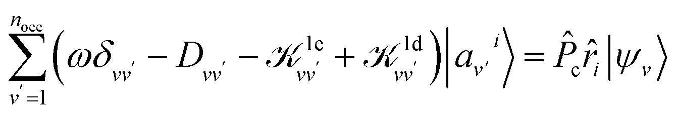
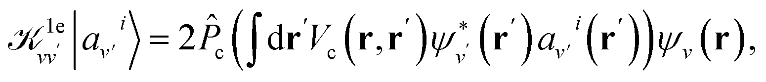
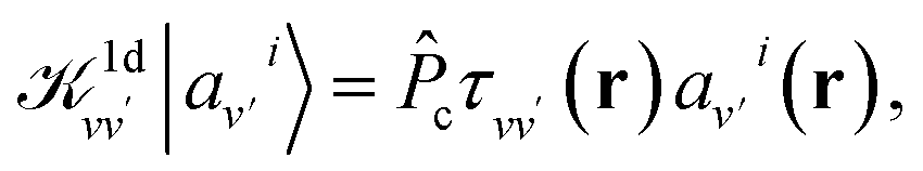
We first briefly summarize the technique used here to solve the BSE, including the use of bisection techniques to improve the efficiency of the method. We then describe the method based on ML to obtain the dielectric screening entering the BSE, including the description of the training set of integrals. These integrals are computed for a chosen configuration of a molecule or a solid.Using the linearized Liouville equation31,35,36,65 and the Tamm–Dancoff approximation,66 the absorption spectrum of a solid or molecule can be computed from DFT38,39 single particles eigenfunctions as:
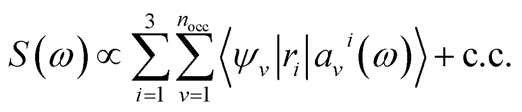 | (1) |
 | (2) |
Dvv′|av′i〉 = ![[P with combining circumflex]](https://www.rsc.org/images/entities/i_char_0050_0302.gif) c(Ĥ0 − εv)δvv′|av′i〉, c(Ĥ0 − εv)δvv′|av′i〉, | (3) |
 | (4) |
 | (5) |
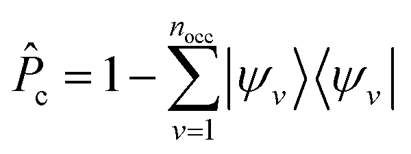 is the projector on the unoccupied manifold, and
  is the unscreened Coulomb potential. Following the derivation reported by Nguyen et al.,31 we defined screened Coulomb integrals, τvv′, entering eqn (5), as:
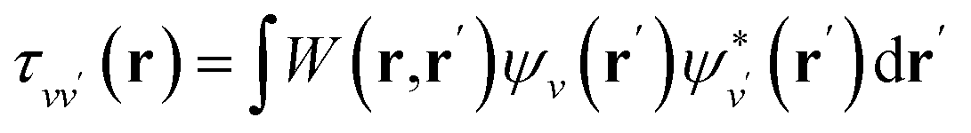 | (6) |
 | (7) |
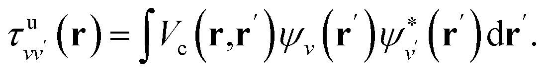 | (8) |
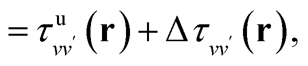
By carrying out finite field calculations,31,37,40 one can obtain screened Coulomb integrals without an explicit evaluation of the dielectric matrix (eqn (6)), but rather by adding to the unscreened Coulomb integrals the second term on the right hand side of eqn (7), which is computed as:
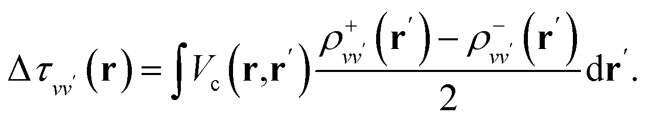 | (9) |
The densities ρ±vv′ are obtained by solving the KS equations with the perturbed Hamiltonian Ĥ ± τuvv′; both indexes v and v′ run over all occupied orbitals. While all potential terms of Ĥ may be computed self-consistently,31 in this work the exchange-correlation potential was evaluated for the initial unperturbed electronic density and kept fixed during the self-consistent iterations. This amounts to evaluating the dielectric screening within the RPA. The FF-BSE approach has been implemented by coupling the WEST18 and Qbox67 codes in client-server mode.31,37,68
The maximum number of integrals, nint = nocc(nocc + 1)/2, is determined by the total number of pairs of occupied orbitals. The actual number of integrals to be evaluated can be greatly reduced by using the recursive bisection method,43 which allows one to localize orbitals and consider only integrals generated by pairs of overlapping orbitals.31 The systems studied in this work contain tens to hundreds of atoms, with hundreds to thousands of electrons. For example, for one of the Si/water interfaces discussed below, we considered a slab with 420 atoms, 1176 electrons and each single particle state is doubly occupied. Hence, nocc = 588, and nint = 173166. Using the recursive bisection method the total number of vv′ pairs is reduced to nint = 5574 (a reduction factor slightly larger than 30) without compromising accuracy, when a bisection threshold of 0.05 and five bisection levels in each Cartesian direction are adopted.43
We note that the Liouville formalism used in this work (eqn (1)) only involves summations over occupied states. Such formalism was shown to yield absorption spectra equivalent to solving the BSE with explicit and converged summations over empty states.31,35,36 The same formalism may also be used to describe absorption spectra within TDDFT,64 albeit employing a different definition of the  and
and  terms.15,31,65,69–72
The key point of our work is the use of ML to generate a model for the calculation of screened Coulomb integrals (eqn (7)) that is transferable to multiple atomic configurations; the goal is to reduce the computational cost in the solution of eqn (1). In particular, we consider the mapping between unscreened Coulomb integrals, τuvv′, and screened Coulomb integrals, Δτvv′. Such transformation is mapping nint pairs of a 3D array, i.e., {F: τuvv′ → Δτvv′,∀v,v′ ∈ [1,…,nocc]} and is similar to 3D image processing. Our objective is to learn the mapping functions and hence it is natural here to use convolutional neural networks (CNN), a widely used technique in image classification. CNNs are artificial neural networks with spatial-invariant features. The screened and unscreened Coulomb integrals are related by the dielectric matrix, which describes a linear response function of the system to an external perturbation. Therefore, the mapping we aim to obtain should follow a linear relationship for physical reasons, and one convolutional layer without nonlinear activation functions should be considered. Here, the surrogate model F, used to bypass the explicit calculation of eqn (9), is represented by a single convolutional layer K:
| Δτvv′(x,y,z) = (K * τuvv′)(x,y,z) | (10) |
The filter, K, is determined through an optimization procedure that utilizes nint pairs of τuvv′ and Δτvv′ as the dataset, obtained for one configuration (i.e., one set of atomic positions) using eqn (8) and eqn (9), respectively. Therefore this filter captures features in the dielectric screening that are translationally invariant. When the filter size is reduced to (1, 1, 1), the training procedure is effectively a linear regression and eqn (10) amounts to applying a global scaling factor to τuvv′, which we label fML.
In our calculations, the mapping F corresponds to evaluating the dielectric screening arising from the short-wavelength part (i.e., the body) of the dielectric matrix. The long-wavelength part (i.e., the head of the dielectric matrix) corresponds to the macroscopic dielectric constant ε∞. The definitions of the head and body of the dielectric matrix are given in eqn (S1) of the ESI.†
One of the main advantages of a ML-based model for the screening is that it may be reused for multiple configurations sampled during a FPMD simulation, thus avoiding the calculations of dielectric matrices for each snapshot, as illustrated in Fig. 1. The validity of such an approach and its robustness are discussed below for several systems. In our calculations, we carried out FPMD with the Qbox67 code and MBPT theory calculations with the WEST18 code, coupled in client server mode with Qbox in order to evaluate the screened integrals (eqn (7–9)), which constitute our training dataset. We implemented an interface between Tensorflow73 and WEST, including a periodic padding of the data for the convolution in eqn (10), in order to satisfy periodic boundary conditions. The computational details of each system investigated here are reported in the ESI.† Data and scripts are available through Qresp at https://paperstack.uchicago.edu/paperdetails/60316fb93f58fc9075286688?server=https%3A%2F%2Fpaperstack.uchicago.edu.74
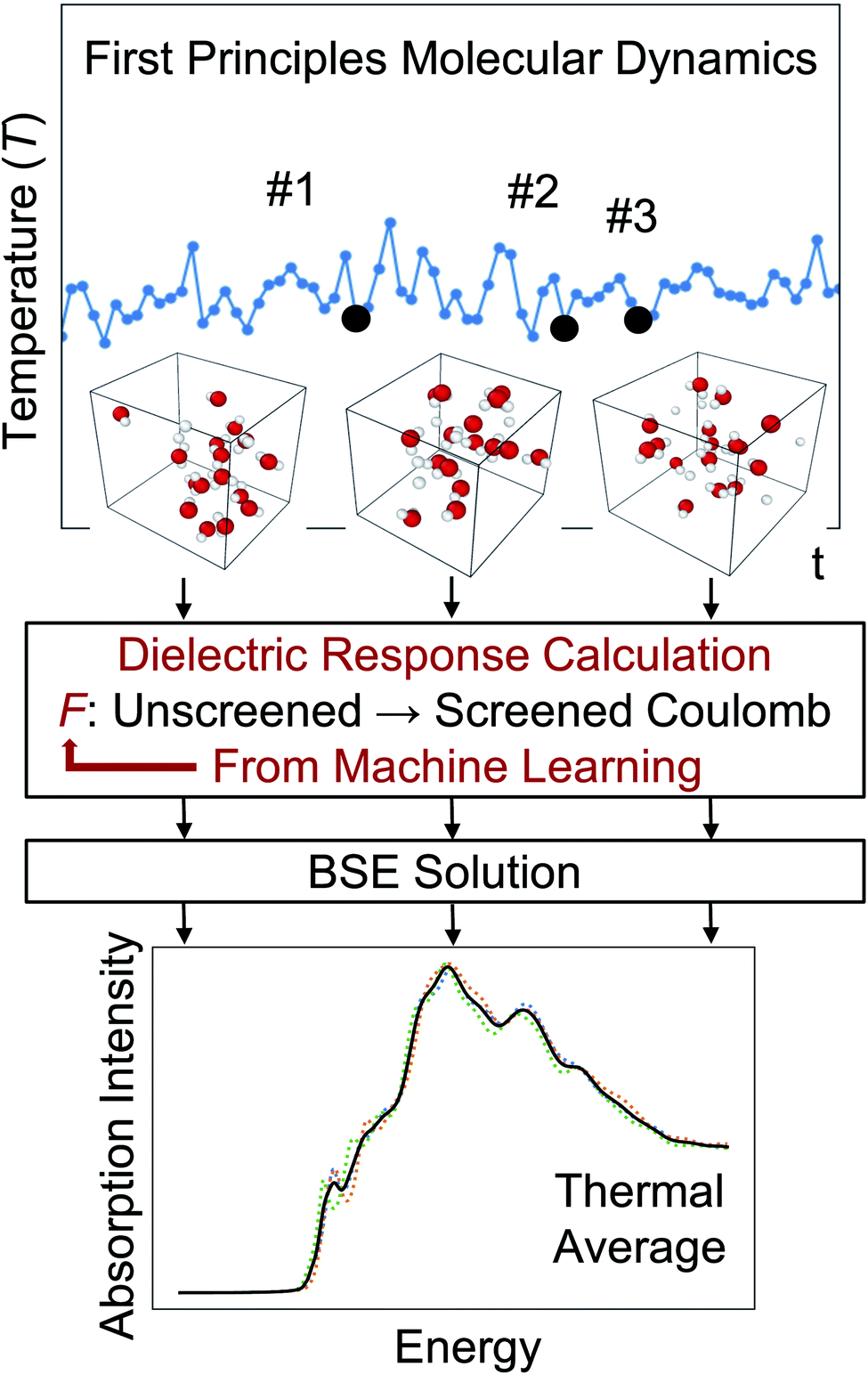 | ||
| Fig. 1 Illustration of the strategy to predict absorption spectra at finite temperature based on the solution of the Bethe–Salpeter equation (BSE) and machine learning techniques. F is the mapping obtained by machine learning. | ||
Results
We now turn to present our results for several systems, starting from liquid water.Liquids
To establish baseline results with small computational cost, we first considered a water supercell containing 16 water molecules. We tested the accuracy of a single convolutional layer with different filter sizes, from (1, 1, 1) to (20, 20, 20). We find that a convolutional model (eqn (10)) can be used to bypass the calculation of Δτ in eqn (9), yielding absorption spectra in good agreement with the FF-BSE method. In particular, we find that a filter size of (1, 1, 1), i.e., a global scaling factor, is sufficient to accurately yield the positions of the lower-energy peaks of the absorption spectra, with an error of only −0.03 eV (see the ESI† for a detailed quantification of the error).We then turned to interpret the meaning of the global scaling factor fML, and we computed the quantity εMLf = (1 + fML)−1. For 20 independent snapshots extracted from a FPMD trajectory of the 16-H2O system, we find that εMLf = 1.84 ± 0.02 is the same, within statistical error bars, as that of the PBE75 macroscopic static dielectric constant computed using the polarizability tensor (as implemented in the Qbox code67): εPT∞ = 1.83 ± 0.01. Therefore, the global scaling factor that we learned is closely related to the long-wavelength dielectric constant of the system. Interestingly, we obtained similar scaling factors for a simulation using a larger cell, with 64-molecules, e.g., εMLf = 1.83 for a given, selected snapshot, for which εPT∞ = 1.86. To further interpret the factor fML obtained by ML, we computed the average of Δτvv′/τuvv′ over all vv′. Specifically, we define 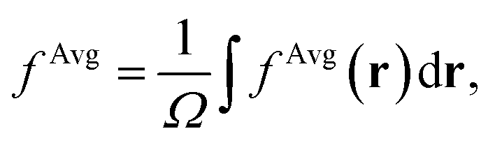 where
where 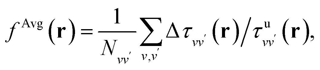 Ω is the volume of the simulation cell, and Nvv′ is the total number of vv′ in the summation. Using one snapshot of the 16-H2O system as an example, we find that εAvgf = (1 + fAvg)−1 = 1.79, similar to εMLf = 1.86 for the same snapshot.
To evaluate how sensitive the peak positions in the absorption spectra of water are to the value of the global scaling factor, we varied εf from 1.67 to 1.92. We find that the position of the lowest-energy peak varies approximately in a linear fashion, from 8.69 eV to 8.76 eV. This analysis shows that a global scaling factor is sufficient to represent the average effect of the body (i.e., short-wavelength part) of the dielectric matrix and that this factor is approximately equal to the head of the matrix (related to the long-wavelength dielectric constant). Hence, our results show that a diagonal dielectric matrix is a sufficiently good approximation to represent the screening of liquid water and to obtain its optical spectrum by solving the BSE. This simple finding is in fact an important result, leading to a substantial reduction in the computational time necessary to obtain the absorption spectrum of water at the BSE level of theory.
In order to understand how the screening varies over a FPMD trajectory, we applied the global scaling factor fML obtained from one snapshot of the 16-H2O system to 10 different snapshots of a 64-H2O system,76 at the same T, 400 K, and we computed an average spectrum. As shown in Fig. 2, we can accurately reproduce the average spectrum computed with FF-BSE. The RMSE between the two spectra is 0.027. These results show that the global scaling factor is transferable from the 16 to the 64 water cell and that the dependence of the global scaling factor on the atomic positions may be neglected, for the thermodynamic conditions considered here. While it was recognized that the dielectric constant of water is weakly dependent on the cell size, it was not known that the average effect of the body of the dielectric matrix is also weakly dependent on the cell size. In addition, our results show that the dielectric screening can be considered independent from atomic positions for water at ambient conditions. This property of the dielectric screening was not previously recognized; it is not only an important recognition from a physical standpoint, but also from an efficiency standpoint, to improve the efficiency of BSE calculations.
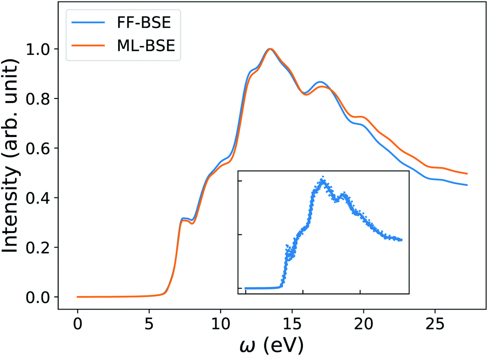 | ||
| Fig. 2 Averaged spectra of liquid water obtained by solving the Bethe–Salpeter equation (BSE) in finite field (FF) and using machine learning techniques (ML). Results have been averaged over 10 snapshots obtained from first principles simulations at 400 K, using supercells with 64 water molecules. The variability of the FF-BSE spectra within the 10 snapshots is shown in the inset. See also Fig. S4 of the ESI† for the same variability when using ML-BSE. | ||
The timing acceleration of ML-BSE compared to FF-BSE is a function of the size of the system (characterized by the number of screened integrals nint and the number of plane waves (PWs) npw). We denote by td the total number of core hours required to compute the net screening Δτ for all pairs of orbitals. We do not include in td the training time, which usually takes only several minutes on one GPU for the systems studied here. Since we perform the training procedure once, we consider the training time to be negligible. We define the acceleration to compute the net effect of the screening as αd = tFF-BSEd/tML-BSEd, and we find that αd increases as nint and npw increase. See the ESI† for details.
For the 64-H2O system discussed above, we used a bisection threshold equal to 0.05, and a bisection level of 2 for each of the Cartesian direction. This reduces nint from 256(256 + 1)/2 = 32896 to 3303. In this case, the gain achieved with our machine learning technique is close to two orders of magnitude: αd = 87.
Solids
We now turn to discussing the accuracy of ML-BSE for several solids, including LiF, MgO, Si, SiC, and C (diamond), for which we found again remarkable efficiency gains, ranging from 13 to 43 times for supercells with 64 atoms. In all cases, we used the experimental lattice constants.77 Similar to water, we found that a convolutional model (eqn (10)) can reproduce the absorption spectra of solids at the FF-BSE level, and that global scaling factors, either from linear regression or from averaging Δτ/τu yield similar accuracy (Fig. S6 snd S7 of the ESI†). As shown in Fig. 3, where we have defined fPT = (εPT∞)−1 − 1, we found that fML is again numerically close to fPT, for εPT∞ computed using the polarizability tensor,67 and the same level of theory and k-point sampling. These results show that, for ordered solids, the average effect of the body (short-wavelength part) of the dielectric matrix, εMLf, is similar to that of the head (long-wavelength limit) of the matrix and hence a diagonal screening is sufficient to describe the absorption spectra, similar to the case of water. This is an interesting result that supports the validity of the approximation chosen to derive the DDH functional.44–46,78–83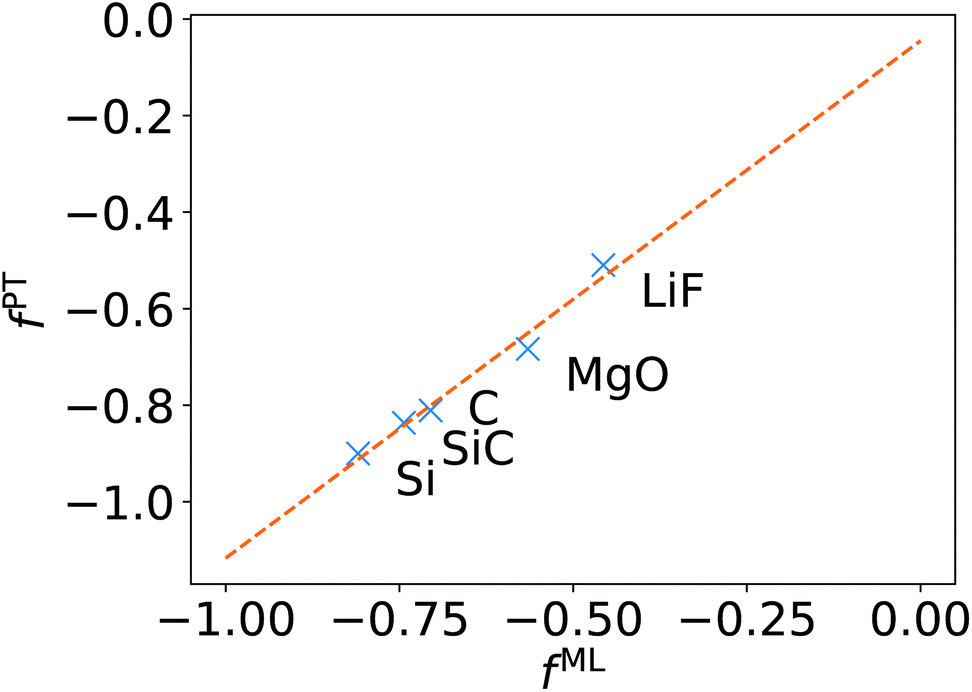 | ||
| Fig. 3 Relationship between the scaling factor obtained by machine learning (fML) and that obtained by computing the dielectric constant at the same level of theory (fPT) (see text). | ||
We note that the FF-BSE algorithm uses the Γ point and is efficient and appropriate for large systems. In order to verify that a diagonal dielectric matrix is an accurate approximation also when using unit cells and fine grids of k-points, we computed the absorption spectrum of Si with a 2-atom cell and a 12 × 12 × 12 k-point grid, using the Yambo84,85 code. We then compared the results with those obtained using a diagonal approximation of the dielectric matrix, and elements derived from the long-wavelength dielectric constant computed with the same cell and k-point grid. Fig. 4 shows that we found an excellent agreement between the two calculations, of the same quality as that obtained for water in the previous section.
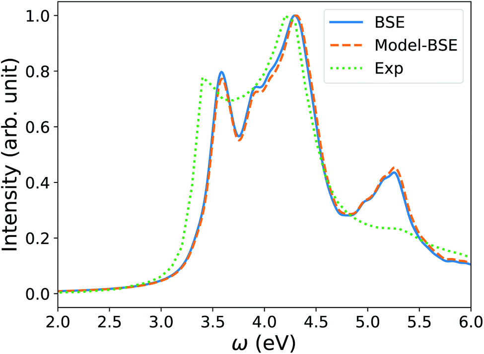 | ||
| Fig. 4 Absorption spectrum of crystalline Si computed by solving the Bethe–Salpeter equation (BSE) starting from PBE75 wavefunctions, using a 2-atom cell and 12 × 12 × 12 k-point sampling (blue line). The orange dashed line (Model-BSE) shows the same spectrum computed using a diagonal dielectric matrix with diagonal elements equal to ε∞ = 12.21 (see text). Experimental results86 are shown by the green dotted line. | ||
It is important to note that the method presented here to learn the filter between unscreened and screened integrals represents a way of obtaining a model dielectric function with ML techniques, and without the need of using ad hoc empirical parameters. Several model dielectric functions have been proposed to speed-up the solution of the BSE for solids over the years.48,87–93 Recently, Sun et al.48 proposed a simplified BSE method that utilizes a model dielectric function (m-BSE). The authors used the model of Cappellini et al.91 with an empirical parameter, which they determined by averaging the values minimizing the RMSE between a model dielectric function and that obtained within the RPA for Si, Ge, GaAs, and ZnSe.94 This simplified BSE method yields good agreement with the results of the full BSE solution. For example, in the case of LiF, the shift between the first peak obtained with m-BSE and BSE is 0.12 eV, to be compared to the shift of 0.04 eV found here, between ML-BSE and FF-BSE. A model dielectric function has been proposed also for 2D semiconductors95 and silicon nanoparticles.96,97 However, the important difference between our work and the models just described is that the latter requires empirical parameterization. One of the advantages of the ML approach adopted here is that it does not require the definition of empirical parameters and, importantly, it may also be applied to nanostructures and heterogeneous systems, such as solid/liquid interfaces, as discussed next.
Interfaces
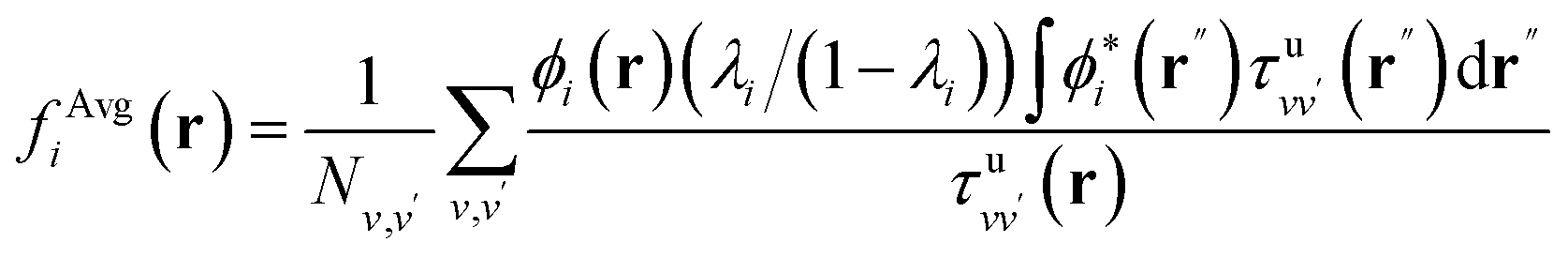
We have shown that for solids and liquids, the use of ML leads to the definition of a global scaling factor that, when utilized to model the screened Coulomb interaction, yields results for absorption spectra in very good agreement with those of the full FF-BSE calculations, at a much lower computational cost. We now discuss solid/liquid interfaces as prototypical heterogeneous systems.We considered two silicon/water interfaces modeled by periodically repeated slabs. One is the H–Si/water interface, a hydrophobic interface with 420 atoms (72 Si atoms and 108 water molecules; Si surface capped by 24 H atoms); the other is a COOH–Si/water interface, a hydrophilic interface with 492 atoms (72 Si atoms and 108 water molecules; Si surface capped by 24 –COOH groups).98 Not unexpectedly, we found that neither a global scaling factor nor a convolutional model is sufficiently accurate to reproduce the spectra obtained with FF-BSE, as shown in Fig. S11 of the ESI.† Therefore, we have developed a position-dependent ML model to describe the variation of the dielectric properties in the Si, water and interfacial regions. We divided the grid of τvv′ into slices, each spanning one xy plane parallel to the interface; we then trained for a model on each slice. In this way we describe translationally invariant features along the x and y directions, and we obtain a z-dependent convolutional filter K(z) or z-dependent scaling factors fML(z). We found that a position-dependent filter, K(z), or a scaling factor for each slice, fML(z), yield a comparable accuracy, and therefore we focus on the fML(z) model, which is simpler.
We found that the z-dependent ML model fML(z) is accurate to represent the screening of the Si/water interfaces when computing absorption spectra (Fig. 5). Together with Fig. S11 in the ESI,† our finding show that a block diagonal dielectric matrix, where all the diagonal elements in the dielectric matrix have the same value, is not a good representation of the screening, unlike the case of water and ordered, periodic solids; instead taking into account the body of the dielectric matrix as in the fML(z) model is critical in the case of an interface.
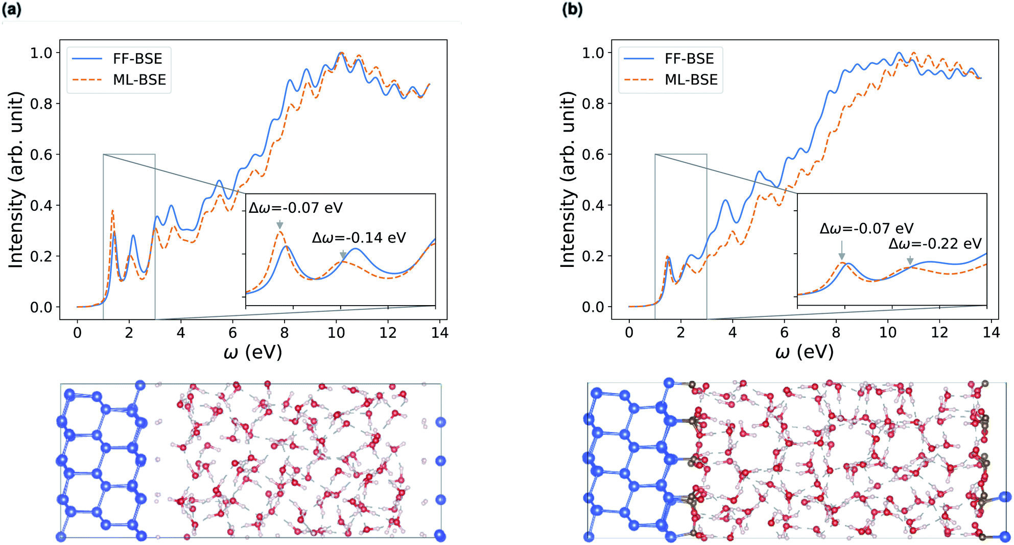 | ||
| Fig. 5 Comparison of absorption spectra obtained by solving the Bethe–Salpeter equation (BSE) in finite field (FF) and using machine learning (ML) techniques for (a) a H–Si/water interface shown in the lower left panel and (b) a COOH–Si/water interface (shown in the lower right panel). Blue, red and white spheres represent Si, oxygen and hydrogen respectively. C is represented by brown spheres. (See the ESI† for results from using a kinetic energy cutoff of 60 Ry for wavefunctions.). | ||
Depending on how the grid of τvv′ are divided, we obtain different fML(z) profiles for Si/water interfaces. Fig. 5 shows the spectra in the case of fML(z) defined by two parameters (a constant value in the Si region, and a different constant value in the water region); we name this profile fMLp2(z). In Fig. S12(a) of the ESI,† we present the spectra obtained using fML(z) in the case of 108 slices evenly spaced in the z direction, which we call fMLp108(z). The function εMLf(z) corresponding to fMLp108(z) presents maxima at the interfaces, and minima at the points furthest away from the interface, in the Si and the water regions (Fig. S12(b) of the ESI†).
In order to interpret our findings, we express Δτ in terms of projective dielectric eigenpotentials, (PDEP)99,100 and we decompose fAvg(r) into contributions from each individual PDEP,101i.e., 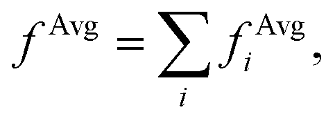 where
where
 | (11) |
Interestingly, fMLp2(z) and fMLp108(z) yield absorption spectra of similar quality. This suggests that the absorption spectrum is not sensitive to the details of the profile at the interface, at least in the case of the H–Si/water interface (Fig. 5(a) and S12 of the ESI†) and the COOH–Si/water interface (Fig. 5(b) and S16 of the ESI†) studied here. However, knowing the functional form of fMLp108(z) is useful to determine the location of the interfaces, and it can be used to define where the discontinuities in fMLp2(z) are located.
We further developed a 3D grid model, fML(r). This is a simple extension of the z-dependent model, where instead of slicing τvv′ in only one direction, we equally divided τvv′ into sub-domains in all three Cartesian directions. We tested cubic sub-domains of side lengths from 0.6 Å to 2.6 Å, and we found that the accuracy of the resulting spectrum is similar to that obtained with the z-dependent model, as shown in Fig. S14 of the ESI.†
In order to verify the transferability of the position-dependent model derived for one snapshot extracted from FPMD to other snapshots, we computed absorption spectra by using the same fML(z) for different snapshots generated at ambient conditions and we found that the screening is weakly dependent on the atomic positions, at these conditions, similar to the case of water discussed above (Fig. S15 of the ESI†).
In summary, by obtaining εMLf(z) from machine learning, we have provided a way to define a position-dependent dielectric function for heterogeneous systems. For the Si/water interfaces, the acceleration to compute the net screening effect is αd = 86 for H–Si/water if bisection techniques are used (nint = 5574), and αd = 224 for COOH–Si/water, again if bisection techniques are used (nint = 8919).
Nanoparticles
As our last example we consider nanoparticles, i.e., 0D systems. We focus on silicon clusters Si35H36 and Si87H76 (ref. 18, 81 and 102) but we start from a small cluster Si10H16 first, to test the methodology. As shown in Fig. 6(b), we found that a global scaling factor is not an appropriate approximation of the screening, e.g., for the spectrum of Si10H16 computed using PW basis set in a simulation cell with a large vacuum (cell length over 25 Å). This finding points at an important qualitative difference with respect to the case of solids and liquids (condensed systems). Interestingly, we found that convolutional models are instead robust to different sizes of vacuum, and give absorption spectra in good agreement with FF-BSE calculations (Fig. 6(a)). The inaccuracy of a global scaling factor stems from two reasons. One is related to the fact that when the volume of the vacuum surrounding the cluster becomes large, the data of the training set is dominated by small matrix elements representing the vacuum region. Because the numerical noise is not translationally invariant, the use of eqn (10) overcomes this issue, as the noise from vacuum matrix elements is canceled out in the convolution process. We note that the presence of nonzero elements in the vacuum region is due to the choice of the PW basis set, which requires periodic boundary conditions. In the case of isolated clusters, the use of periodic boundary conditions could be avoided by choosing localized basis set. However, there are several systems of interest where using PW basis set is preferable and vacuum regions are present, such as nanoparticles deposited on surfaces. The second reason responsible for the inaccuracy of a global scaling factor, even if the noise arising from vacuum is eliminated, (see Fig. S18 of the ESI†), is that the mapping between τu and Δτ being is simply more complex in nanoparticles than in homogeneous systems. Such a complexity can be accounted for when using eqn (10).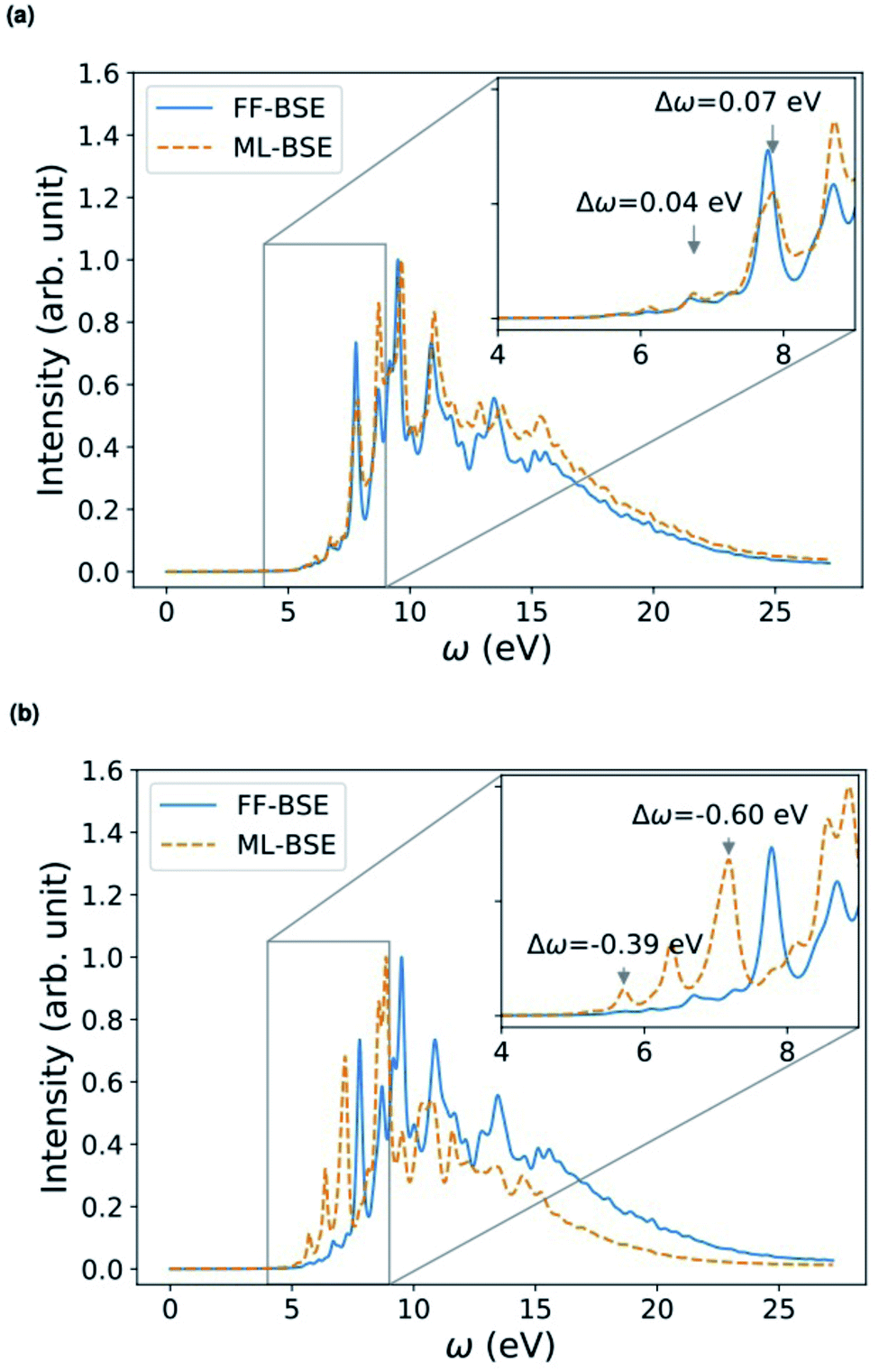 | ||
| Fig. 6 Comparison of absorption spectra of Si10H16 (40 Å cell) obtained by solving the Bethe–Salpeter equation (BSE) in finite field (FF) and using machine learning (ML) techniques for (a) convolutional layer with filter size (7, 7, 7) from a cell of 30 Å, and (b) a global scaling factor. The RMSE value between the FF-BSE and ML-BSE spectra is 0.067 for (a) and 0.141 for (b), respectively. The accuracy of using a convolutional layer with filter size (7, 7, 7) from the 40 Å cell itself is similar to that of (a): RMSE = 0.067. | ||
In order to investigate the dependence of the screening of nanoparticles on temperature, we transferred the ML model trained for one specific snapshot of the Si35H36 cluster, to different snapshots extracted from a FPMD simulation, in order to predict absorption spectra at finite temperature. We applied the convolutional model with filter size (7, 7, 7) obtained from the 0 K Si35H36 cluster to 10 snapshots of Si35H36 from an FPMD trajectory equilibrated at 500 K. As shown in Fig. 7, the average ML-BSE spectrum can accurately reproduce the FF-BSE absorption spectrum at 500 K, with a small peak position shift of 0.08 eV. The ML-BSE spectra of individual snapshots is also in good agreement with the corresponding spectra computed with FF-BSE, shown in Fig. S22 of the ESI.† These results show that for nanoclusters, as for water, the screening is weakly dependent on atomic positions over a 500 K FPMD trajectory; note however that the 0 K spectrum (Fig. S20 of the ESI†) has different spectral features than the one collected at 500 K (Fig. 7).
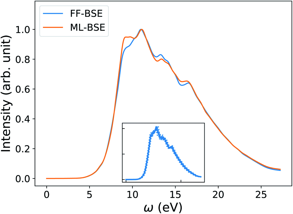 | ||
| Fig. 7 Average spectra of Si35H36 obtained by solving the Bethe–Salpeter equation (BSE) in finite field (FF) and using machine learning techniques (ML). Results have been averaged over 10 snapshots obtained from first principles simulations at 500 K. The variability of the FF-BSE spectra within the 10 snapshots is shown in the inset. See also Fig. S21 of the ESI† for the same variability when using ML-BSE. | ||
We also found that the convolutional model trained for Si35H36 can be applied to Si87H76 with an error within 0.07 eV for peak positions (Fig. 8). The accuracy is comparable to the convolutional model from Si87H76 itself, as shown in Fig. S24 of the ESI.† This shows that the convolutional model captures the nonlocality of the dielectric screening common to Si clusters of different sizes and is transferable from a smaller to a larger nanocluster (Si87H76) within the size range considered here. The FF-BSE calculation of Si87H76 is about 6 times more expensive in terms of core hours than that of Si35H36; hence, being able to circumvent the FF-BSE calculation of Si87H76 by using the model K computed for Si35H36 is certainly an advantage.
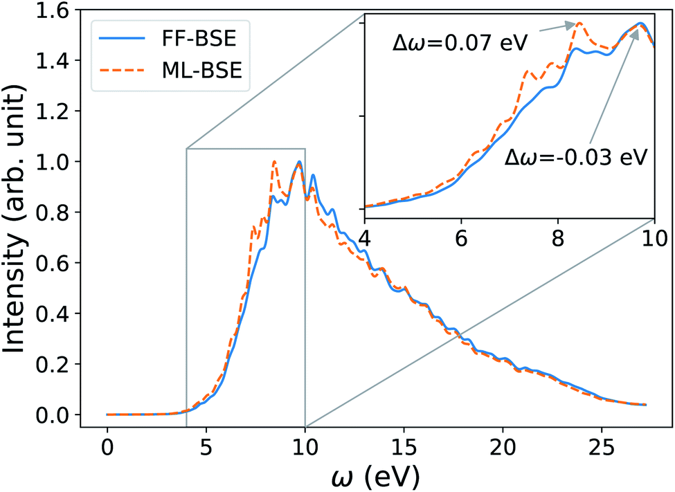 | ||
| Fig. 8 Accuracy of the Si87H76 spectrum obtained from ML-BSE by applying a convolutional model with filter size (7, 7, 7), trained from Si35H36. The RMSE value between the FF-BSE and ML-BSE spectra is 0.033. | ||
Conceptually, the convolutional model yields filters that capture the translational invariant features of the dataset, and in our case they capture the nonlocality of the screening. In other words, the convolutional filters represent features in the mapping from τuvv′ to Δτvv′ that are invariant across the simulation cell. For Si clusters, we found that the RMSE values between ML-BSE and FF-BSE spectra converges as the size of the filter increases. For example, for Si35H36, convergence is achieved at the filter size (7, 7, 7), which corresponds to a cube with side length (2.24 Å), corresponding approximately to the Si–Si bond length in the cluster (2.35 Å). This result suggests that the screening of the Si cluster has features of the length of a nearest-neighbor bond that are translationally invariant.
The timing acceleration αd for calculations of the absorption spectra of the Si35H36 cluster in a cubic cell of 20, 25, or 30 Å in length, is 24, 47, or 90 times, respectively, when using bisection techniques (threshold 0.03, 4 levels in each Cartesian direction), as shown in Fig. S25 of the ESI.† In the case of Si87H76 cluster, αd ≃ 160.
Conclusions
We presented a method based on machine learning (ML) to determine a key quantity entering many body perturbation theory calculations, the dielectric screening; this quantity determines the strength of the electron–hole interaction entering the BSE. In our ML model, the screening is viewed as a convolutional (linear) filter that transforms the unscreened into the screened Coulomb interaction. Our results show that such a model can be obtained for a chosen atomic configuration and then re-used to represent the screening of multiple configurations sampled in a FPMD at finite temperature for several systems, including water, solid/water interfaces, and silicon clusters.In particular, we found that in the case of homogeneous systems, e.g. liquid water and several insulating and semiconducting solids, absorption spectra can be accurately predicted by using a diagonal dielectric matrix. When using such a diagonal form, we found excellent agreement with spectra computed by the full solution of the BSE in finite field. In addition, our results showed that for liquid water the same diagonal approximation can be used to accurately compute spectra for different configurations from FPMD at ambient conditions, thus easily obtaining a thermal average representing a finite temperature spectrum.
In the case of nanostructures and heterogeneous systems, such as solid/liquid interfaces, we found that the use of diagonal matrices or block-diagonal dielectric matrices to describe the two portions of the system (Si and water, in the example chosen here) does not yield accurate spectra; through machine learning of the screening we could define simple models yielding accurate absorption spectra and a simple way of computing thermal averages. For nanostructures, it is necessary to use a convolutional model to properly represent the nonlocality of the dielectric screening. Similar to water and the Si/water interfaces, we found that the function describing the screening for hydrogenated Si-clusters of about 1 nm does not depend in any substantial way on the atomic coordinates of the snapshots sampled during our FPMD simulations, up to the maximum temperature tested here, 500 K.
The time savings in the calculations of the screening using ML are remarkable, ranging from a factor of 13 to 87 for the solids and liquids studied here, with cells varying from 64 to 192 atoms. For the clusters and the interface, we obtained time savings ranging from 30 to 224 times, with cells varying from 26 to 492 atoms.
Finally, we note that the ML-based procedure presented here, in addition to substantially speeding up the calculation of spectra, especially at finite T, represents a general approach to derive model dielectric functions, which are key quantities in electronic structure calculations, utilized not only in the solution of the BSE. For example, our approach provides a strategy to develop dielectric-dependent hybrid functionals (DDH)45,80 for TDDFT calculations, as well as an interpretation of the parameters entering model dielectric functions.48,87–89,91,93,96,97 In particular, for homogeneous systems, our findings points at TDDFT with DDH functionals as an accurate method to obtain absorption spectra, consistent with the results of Sun et al.,48 which were however derived semi-empirically. Work is in progress to further develop a strategy to develop parameters entering hybrid DFT functionals using machine learning.103
Conflicts of interest
There are no conflicts to declare.Acknowledgements
The authors thank Bethany Lusch, He Ma, Misha Salim, and Huihuo Zheng for helpful discussions. The work was supported by Advanced Materials for Energy-Water Systems (AMEWS) Center, an Energy Frontier Research Center funded by the U.S. Department of Energy, Office of Science, Basic Energy Sciences (DOE-BES), and Midwest Integrated Center for Computational Materials (MICCoM) as part of the Computational Materials Science Program funded by DOE-BES. This research used resources of the Argonne Leadership Computing Facility, which is a DOE Office of Science User Facility supported under Contract DE-AC02-06CH11357, and resources of the University of Chicago Research Computing Center (RCC). The GM4 cluster at RCC is supported by the National Science Foundation's Division of Materials Research under the Major Research Instrumentation (MRI) program award no. 1828629.Notes and references
- E. E. Salpeter and H. A. Bethe, Phys. Rev., 1951, 84, 1232–1242 CrossRef.
- L. Hedin, Phys. Rev., 1965, 139, A796 CrossRef.
- W. Hanke and L. Sham, Phys. Rev. B: Condens. Matter Mater. Phys., 1980, 21, 4656 CrossRef CAS.
- G. Onida, L. Reining, R. Godby, R. Del Sole and W. Andreoni, Phys. Rev. Lett., 1995, 75, 818 CrossRef CAS.
- S. Albrecht, G. Onida and L. Reining, Phys. Rev. B: Condens. Matter Mater. Phys., 1997, 55, 10278 CrossRef CAS.
- S. Albrecht, L. Reining, R. Del Sole and G. Onida, Phys. Rev. Lett., 1998, 80, 4510 CrossRef CAS.
- S. Albrecht, L. Reining, R. Del Sole and G. Onida, Phys. Status Solidi A, 1998, 170, 189–197 CrossRef CAS.
- L. X. Benedict, E. L. Shirley and R. B. Bohn, Phys. Rev. Lett., 1998, 80, 4514 CrossRef CAS.
- M. Rohlfing and S. G. Louie, Phys. Rev. Lett., 1998, 81, 2312 CrossRef CAS.
- M. Rohlfing and S. G. Louie, Phys. Rev. B: Condens. Matter Mater. Phys., 2000, 62, 4927 CrossRef CAS.
- X. Blase, I. Duchemin and D. Jacquemin, Chem. Soc. Rev., 2018, 47, 1022–1043 RSC.
- G. Strinati, La Rivista del Nuovo Cimento, 1988, 11, 1–86 CrossRef CAS.
- G. Onida, L. Reining and A. Rubio, Rev. Mod. Phys., 2002, 74, 601–659 CrossRef CAS.
- R. M. Martin, L. Reining and D. M. Ceperley, Interacting electrons, Cambridge University Press, 2016 Search PubMed.
- Y. Ping, D. Rocca and G. Galli, Chem. Soc. Rev., 2013, 42, 2437–2469 RSC.
- M. Govoni and G. Galli, J. Chem. Theory Comput., 2018, 14, 1895–1909 CrossRef CAS.
- D. Golze, M. Dvorak and P. Rinke, Front. Chem., 2019, 7, 377 CrossRef CAS.
- M. Govoni and G. Galli, J. Chem. Theory Comput., 2015, 11, 2680–2696 CrossRef CAS.
- H. Seo, M. Govoni and G. Galli, Sci. Rep., 2016, 6, 1–10 CrossRef.
- A. P. Gaiduk, M. Govoni, R. Seidel, J. H. Skone, B. Winter and G. Galli, J. Am. Chem. Soc., 2016, 138, 6912–6915 CrossRef CAS.
- P. Scherpelz, M. Govoni, I. Hamada and G. Galli, J. Chem. Theory Comput., 2016, 12, 3523–3544 CrossRef CAS.
- H. Seo, H. Ma, M. Govoni and G. Galli, Phys. Rev. Mater., 2017, 1, 075002 CrossRef.
- R. L. McAvoy, M. Govoni and G. Galli, J. Chem. Theory Comput., 2018, 14, 6269–6275 CrossRef CAS.
- T. J. Smart, F. Wu, M. Govoni and Y. Ping, Phys. Rev. Mater., 2018, 2, 124002 CrossRef CAS.
- A. P. Gaiduk, T. A. Pham, M. Govoni, F. Paesani and G. Galli, Nat. Commun., 2018, 9, 1–6 CrossRef CAS.
- M. Gerosa, F. Gygi, M. Govoni and G. Galli, Nat. Mater., 2018, 17, 1122–1127 CrossRef CAS.
- R. Car and M. Parrinello, Phys. Rev. Lett., 1985, 55, 2471 CrossRef CAS.
- V. Garbuio, M. Cascella, L. Reining, R. Del Sole and O. Pulci, Phys. Rev. Lett., 2006, 97, 137402 CrossRef CAS.
- D. Lu, F. Gygi and G. Galli, Phys. Rev. Lett., 2008, 100, 147601 CrossRef.
- L. Bernasconi, J. Chem. Phys., 2010, 132, 184513 CrossRef.
- N. L. Nguyen, H. Ma, M. Govoni, F. Gygi and G. Galli, Phys. Rev. Lett., 2019, 122, 237402 CrossRef CAS.
- M. Marsili, E. Mosconi, F. De Angelis and P. Umari, Phys. Rev. B: Condens. Matter Mater. Phys., 2017, 95, 075415 CrossRef.
- J. D. Elliott, N. Colonna, M. Marsili, N. Marzari and P. Umari, J. Chem. Theory Comput., 2019, 15, 3710–3720 CrossRef CAS.
- F. Henneke, L. Lin, C. Vorwerk, C. Draxl, R. Klein and C. Yang, Comm. App. Math. Comp. Sci., 2020, 15, 89–113 CrossRef.
- D. Rocca, D. Lu and G. Galli, J. Chem. Phys., 2010, 133, 164109 CrossRef.
- D. Rocca, Y. Ping, R. Gebauer and G. Galli, Phys. Rev. B: Condens. Matter Mater. Phys., 2012, 85, 045116 CrossRef.
- H. Ma, M. Govoni, F. Gygi and G. Galli, J. Chem. Theory Comput., 2019, 15, 154–164 CrossRef CAS.
- P. Hohenberg and W. Kohn, Phys. Rev., 1964, 136, B864 CrossRef.
- W. Kohn and L. J. Sham, Phys. Rev., 1965, 140, A1133 CrossRef.
- H. Ma, M. Govoni, F. Gygi and G. Galli, J. Chem. Theory Comput., 2020, 16, 2877–2879 CrossRef CAS.
- H. Ma, M. Govoni and G. Galli, npj Comput. Mater., 2020, 6, 1–8 CrossRef.
- H. Ma, N. Sheng, M. Govoni and G. Galli, Phys. Chem. Chem. Phys., 2020, 22, 25522–25527 RSC.
- F. Gygi, Phys. Rev. Lett., 2009, 102, 166406 CrossRef.
- T. Shimazaki and Y. Asai, J. Chem. Phys., 2009, 130, 164702 CrossRef.
- J. H. Skone, M. Govoni and G. Galli, Phys. Rev. B: Condens. Matter Mater. Phys., 2014, 89, 195112 CrossRef.
- M. Gerosa, C. Bottani, C. Di Valentin, G. Onida and G. Pacchioni, J. Phys.: Condens. Matter, 2017, 30, 044003 CrossRef.
- W. Chen, G. Miceli, G.-M. Rignanese and A. Pasquarello, Phys. Rev. Mater., 2018, 2, 073803 CrossRef CAS.
- J. Sun, J. Yang and C. A. Ullrich, Phys. Rev. Res., 2020, 2, 013091 CrossRef CAS.
- G. Montavon, M. Rupp, V. Gobre, A. Vazquez-Mayagoitia, K. Hansen, A. Tkatchenko, K.-R. Müller and O. A. Von Lilienfeld, New J. Phys., 2013, 15, 095003 CrossRef.
- F. Brockherde, L. Vogt, L. Li, M. E. Tuckerman, K. Burke and K.-R. Müller, Nat. Commun., 2017, 8, 1–10 CrossRef CAS.
- M. Welborn, L. Cheng and T. F. Miller III, J. Chem. Theory Comput., 2018, 14, 4772–4779 CrossRef CAS.
- G. R. Schleder, A. C. M. Padilha, C. M. Acosta, M. Costa and A. Fazzio, JPhys Mater., 2019, 2, 032001 CrossRef CAS.
- K. Ryczko, D. A. Strubbe and I. Tamblyn, Phys. Rev. A, 2019, 100, 022512 CrossRef CAS.
- F. Noé, A. Tkatchenko, K.-R. Müller and C. Clementi, Annu. Rev. Phys. Chem., 2020, 71, 361–390 CrossRef.
- F. Häse, L. M. Roch, P. Friederich and A. Aspuru-Guzik, Nat. Commun., 2020, 11, 1–11 Search PubMed.
- C. Sutton, M. Boley, L. M. Ghiringhelli, M. Rupp, J. Vreeken and M. Scheffler, Nat. Commun., 2020, 11, 1–9 Search PubMed.
- M. Bogojeski, L. Vogt-Maranto, M. E. Tuckerman, K.-R. Müller and K. Burke, Nat. Commun., 2020, 11, 1–11 Search PubMed.
- H. S. Stein, D. Guevarra, P. F. Newhouse, E. Soedarmadji and J. M. Gregoire, Chem. Sci., 2018, 10, 47–55 RSC.
- M. Gastegger, J. Behler and P. Marquetand, Chem. Sci., 2017, 8, 6924–6935 RSC.
- S. Ye, W. Hu, X. Li, J. Zhang, K. Zhong, G. Zhang, Y. Luo, S. Mukamel and J. Jiang, Proc. Natl. Acad. Sci. U. S. A., 2019, 116, 11612–11617 CAS.
- K. Ghosh, A. Stuke, M. Todorović, P. B. Jørgensen, M. N. Schmidt, A. Vehtari and P. Rinke, Adv. Sci., 2019, 1801367 CrossRef.
- M. R. Carbone, M. Topsakal, D. Lu and S. Yoo, Phys. Rev. Lett., 2020, 124, 156401 CrossRef CAS.
- B.-X. Xue, M. Barbatti and P. O. Dral, J. Phys. Chem. A, 2020, 124, 7199–7210 CrossRef CAS.
- E. Runge and E. K. U. Gross, Phys. Rev. Lett., 1984, 52, 997–1000 CrossRef CAS.
- B. Walker, A. M. Saitta, R. Gebauer and S. Baroni, Phys. Rev. Lett., 2006, 96, 113001 CrossRef.
- S. Hirata and M. Head-Gordon, Chem. Phys. Lett., 1999, 314, 291–299 CrossRef CAS.
- F. Gygi, IBM J. Res. Dev., 2008, 52, 137–144 Search PubMed.
- M. Govoni, J. Whitmer, J. de Pablo, F. Gygi and G. Galli, npj Comput. Mater., 2021, 7, 32 CrossRef.
- J. Hutter, J. Chem. Phys., 2003, 118, 3928–3934 CrossRef CAS.
- D. Rocca, R. Gebauer, Y. Saad and S. Baroni, J. Chem. Phys., 2008, 128, 154105 CrossRef.
- O. B. Malcıoğlu, R. Gebauer, D. Rocca and S. Baroni, Comput. Phys. Commun., 2011, 182, 1744–1754 CrossRef.
- X. Ge, S. J. Binnie, D. Rocca, R. Gebauer and S. Baroni, Comput. Phys. Commun., 2014, 185, 2080–2089 CrossRef CAS.
- M. Abadi, A. Agarwal, P. Barham, E. Brevdo, Z. Chen, C. Citro, G. S. Corrado, A. Davis, J. Dean, M. Devin, S. Ghemawat, I. Goodfellow, A. Harp, G. Irving, M. Isard, Y. Jia, R. Jozefowicz, L. Kaiser, M. Kudlur, J. Levenberg, D. Mané, R. Monga, S. Moore, D. Murray, C. Olah, M. Schuster, J. Shlens, B. Steiner, I. Sutskever, K. Talwar, P. Tucker, V. Vanhoucke, V. Vasudevan, F. Viégas, O. Vinyals, P. Warden, M. Wattenberg, M. Wicke, Y. Yu and X. Zheng, TensorFlow: Large-Scale Machine Learning on Heterogeneous Systems, 2015, https://www.tensorflow.org/, Software available from tensorflow.org Search PubMed.
- M. Govoni, M. Munakami, A. Tanikanti, J. H. Skone, H. B. Runesha, F. Giberti, J. de Pablo and G. Galli, Sci. Data, 2019, 6, 190002 CrossRef.
- J. P. Perdew, K. Burke and M. Ernzerhof, Phys. Rev. Lett., 1996, 77, 3865–3868 CrossRef CAS.
- W. Dawson and F. Gygi, J. Chem. Phys., 2018, 148, 124501 CrossRef.
- P. Haas, F. Tran and P. Blaha, Phys. Rev. B: Condens. Matter Mater. Phys., 2009, 79, 085104 CrossRef.
- M. A. Marques, J. Vidal, M. J. Oliveira, L. Reining and S. Botti, Phys. Rev. B: Condens. Matter Mater. Phys., 2011, 83, 035119 CrossRef.
- S. Refaely-Abramson, S. Sharifzadeh, M. Jain, R. Baer, J. B. Neaton and L. Kronik, Phys. Rev. B: Condens. Matter Mater. Phys., 2013, 88, 081204 CrossRef.
- J. H. Skone, M. Govoni and G. Galli, Phys. Rev. B: Condens. Matter Mater. Phys., 2016, 93, 235106 CrossRef.
- N. P. Brawand, M. Vörös, M. Govoni and G. Galli, Phys. Rev. X, 2016, 6, 041002 Search PubMed.
- N. P. Brawand, M. Govoni, M. Vörös and G. Galli, J. Chem. Theory Comput., 2017, 13, 3318–3325 CrossRef CAS.
- T. A. Pham, M. Govoni, R. Seidel, S. E. Bradforth, E. Schwegler and G. Galli, Sci. Adv., 2017, 3, e1603210 CrossRef.
- A. Marini, C. Hogan, M. Grüning and D. Varsano, Comput. Phys. Commun., 2009, 180, 1392–1403 CrossRef CAS.
- D. Sangalli, A. Ferretti, H. Miranda, C. Attaccalite, I. Marri, E. Cannuccia, P. Melo, M. Marsili, F. Paleari and A. Marrazzo, et al. , J. Phys.: Condens. Matter, 2019, 31, 325902 CrossRef CAS.
- D. E. Aspnes and A. Studna, Phys. Rev. B: Condens. Matter Mater. Phys., 1983, 27, 985 CrossRef CAS.
- D. R. Penn, Phys. Rev., 1962, 128, 2093 CrossRef CAS.
- Z. H. Levine and S. G. Louie, Phys. Rev. B: Condens. Matter Mater. Phys., 1982, 25, 6310–6316 CrossRef CAS.
- M. S. Hybertsen and S. G. Louie, Phys. Rev. B: Condens. Matter Mater. Phys., 1988, 37, 2733–2736 CrossRef.
- S. Baroni and R. Resta, Phys. Rev. B: Condens. Matter Mater. Phys., 1986, 33, 7017–7021 CrossRef CAS.
- G. Cappellini, R. Del Sole, L. Reining and F. Bechstedt, Phys. Rev. B: Condens. Matter Mater. Phys., 1993, 47, 9892–9895 CrossRef.
- A. B. Djurišić and E. H. Li, J. Appl. Phys., 2001, 89, 273–282 CrossRef.
- M. Bokdam, T. Sander, A. Stroppa, S. Picozzi, D. D. Sarma, C. Franchini and G. Kresse, Sci. Rep., 2016, 6, 28618 CrossRef CAS.
- J. P. Walter and M. L. Cohen, Phys. Rev. B: Solid State, 1970, 2, 1821 CrossRef.
- M. L. Trolle, T. G. Pedersen and V. Véniard, Sci. Rep., 2017, 7, 39844 CrossRef CAS.
- L.-W. Wang and A. Zunger, Phys. Rev. Lett., 1994, 73, 1039 CrossRef CAS.
- R. Tsu, D. Babić and L. Ioriatti Jr, J. Appl. Phys., 1997, 82, 1327–1329 CrossRef CAS.
- T. A. Pham, D. Lee, E. Schwegler and G. Galli, J. Am. Chem. Soc., 2014, 136, 17071–17077 CrossRef CAS.
- H. F. Wilson, F. Gygi and G. Galli, Phys. Rev. B: Condens. Matter Mater. Phys., 2008, 78, 113303 CrossRef.
- H. F. Wilson, D. Lu, F. Gygi and G. Galli, Phys. Rev. B: Condens. Matter Mater. Phys., 2009, 79, 245106 CrossRef.
- H. Zheng, M. Govoni and G. Galli, Phys. Rev. Mater., 2019, 3, 073803 CrossRef CAS.
- M. Govoni, I. Marri and S. Ossicini, Nat. Photonics, 2012, 6, 672–679 CrossRef CAS.
- S. Dick and M. Fernandez-Serra, Nat. Commun., 2020, 11, 1–10 Search PubMed.
Footnotes |
| † Electronic supplementary information (ESI) available: Computational details, ESI tables and figures. See DOI: 10.1039/d1sc00503k. |
| ‡ Current address: Department of Chemistry and Chemical Biology, Northeastern University, Boston, MA 02115, USA. |
| This journal is © The Royal Society of Chemistry 2021 |