From illumination to prediction: a kinetic model for photoredox catalytic activity

Abstract

Photocatalysis is a powerful tool in synthesis, although the key factors that determine its performance are not fully understood. We present a kinetic model for evaluating photocatalytic performance that can be used both to interpret experiments and to optimize kinetic parameters based on experimental data. We introduce the steady-state reduction potential of the substrate or quencher Q (E_Q) as the descriptor of photocatalytic efficiency. The model relies on key parameters, such as the ground and excited state standard reduction potentials of the photocatalyst (PC) and Q, the reorganization energy, and excitation properties. The model is based on three reversible reactions: excitation of the PC, electron transfer (ET) between Q and the ground state PC, ET between Q and the excited state PC* and an irreversible unproductive PC* + Q → PC + Q step, capturing several key geminate processes. The dependence of E_Q on the standard ground and excited state reduction potentials of the PCs shows that photocatalytic performance is strongly influenced by whether the individual ET steps occur in the Marcus normal or inverted regions. The two-dimensional plot of this function reveals the directions in which the standard ground and excited state reduction potentials should be tuned to enhance photocatalytic performance; these directions are often counterintuitive. The model incorporates cage escape, and we show that it can be treated without introducing additional kinetic substeps. An important finding is that none of the input parameters alone can reliably predict photocatalytic efficiency; this also highlights the significance of the proposed measure E_Q. The model also predicts reduction potential combinations where chemiluminescence is expected. The model is benchmarked against transient and stationary experimental data, demonstrating its ability to recover key kinetic parameters. The model is freely available on GitHub and can be easily extended to incorporate additional processes, making it a versatile tool for qualitative assessment and systematic exploration of emerging photocatalytic strategies.

---

Introduction

Molecular photoredox catalysis is a continuously growing field in chemistry.¹ Photocatalysis harnesses the increased oxidation and reduction power of the photocatalyst (PC) in its excited state formed via absorption of photons, optimally at the visible region. The most common mechanism is the single electron transfer between the excited photocatalyst (PC*) and the reactant or an intermittent quencher (Q). It provides radical intermediates to enable a wide range of transformations that are inaccessible or inefficient under conventional conditions.

A large variety of approaches are employed to obtain insight into the mechanism of molecular photocatalyis.^1b,2 The most important methods are time-resolved spectroscopic techniques, particularly transient absorption spectroscopy,^2d,3 electrochemical methods⁴ as well as chemical probes (e.g. radical clocks, quenching probes),⁵ trapping agents^1c,6 or stoichiometric experiments.⁷

Despite significant advancements in photoredox catalysis, the prediction of reaction rates, selectivity and the influence of system parameters are challenging, as many aspects of the process still remain poorly understood. In fact, photocatalytic efficiency depends on the combined effect of various factors such as the excitation spectrum and the standard ground and excited state reduction potentials of the PC, redox properties of the reactant or the quencher, properties of the solvent, as well as on technical details, such as the illumination design (e.g. lamp intensity or the range of the applied wavelengths).⁸ The correct way to account for the interplay of these factors is to integrate them into a suitable mechanistic framework and build kinetic models to provide a quantitative overview with predictive power.^1b,9 Most models are developed by applying a combination of steady-state photochemistry, transient laser spectroscopy, electrochemistry and electronic structure calculations to obtain kinetic parameters for a particular type of reaction or PC. This limitation on scope is due to the complexity of these techniques, especially if time-resolved properties are pursued (see e.g. ref. 10). In addition, as rate constants are determined by empirical fitting to experimental data, the number of kinetic equations is also limited by data availability, i.e., most side reactions are excluded.

The fundamental equation which must be included in a kinetic model is the electron transfer between the photocatalyst and a quencher or reactant. While it is possible to measure electron transfer rates directly,¹¹ the use of Marcus theory¹² eliminates the need for advanced experimental techniques while providing molecular level insight. It can also be applied to cage escape, which has recently become the center of attention.¹³ The trends also indicate a shift from one-dimensional approaches—where individual parameters are examined independently—to multi-dimensional frameworks capable of capturing the mutual interdependencies among variables.¹⁴ These models are expected to have higher predictive power for a larger reaction scope. For example, the model of Bloh was developed for heterogeneous catalysis with large emphasis on capturing the effect of light intensity¹⁴ but the same model with some simplifications can also be used for homogeneous catalysis. Interestingly, electron transfer is treated there by a simple rate constant instead of Marcus theory and cage escape is included implicitly through the combined effect of a quantum yield parameter introduced for PC* formation and the recombination rate constant. Recent kinetic studies by Swierk and co-workers have shown that the key excited-state quenching and electron-transfer steps can be captured with compact kinetic schemes that successfully rationalize photocatalytic behavior across full cycles.^1b,2b,2g,15

In this study, we aim to develop a general photokinetic model for quantitative prediction of photocatalytic performance. This model is designed to guide the development of new photocatalysts by describing the kinetics of a typical photoredox catalytic sequence. We model the oxidative quenching scenario, where photocatalyst PC transfers an electron to quencher Q after irradiation. The analogous kinetic model for reductive quenching can be derived in a straightforward manner and the final kinetic equations to solve are the same. The inputs are the initial concentrations of PC and Q in their ground states in a given solvent, and the intensity of the incoming beam of light. Q is characterized by its standard ground state reduction potential, whereas PC is characterized by its standard ground state and excited state reduction potentials. The performance of PC under standardized conditions is quantified by E_Q, the steady-state reduction potential of Q. In the present scheme the more negative the predicted steady-state reduction potential of Q the more powerful the PC. We show how the photocatalytically relevant parameters influence the steady-state reduction potential E_Q and how the model can help identify ways to improve photocatalytic performance. To demonstrate its practical relevance, the model is applied to a set of existing photocatalysts characterized in the literature; and we also show how effectively it can be used to fit kinetic parameters to experimental data.

Constructing the kinetic model

Our kinetic formulation is based on the standard excitation and electron-transfer (ET) steps broadly employed in PC/Q models, e.g. in the analyses of Swierk and co-workers. These steps can be treated as reversible when required by thermodynamic considerations, preserving the conventional model architecture while allowing additional flexibility. Hence the following equations are defined:

The key innovation is the addition of an effective step to capture nonproductive solvent-cage dynamics which prior models treated only implicitly. This assumes that a solvent cage containing an initial encounter complex of P* and Q is formed and ET takes place within this cage.¹³ Then, the competition between diffusive escape in eqn (4) and geminate recombination in eqn (5) determines whether Q⁻ can contribute productively to the subsequent photocatalytic process or PC⁺ and Q⁻ are quenched to PC + Q through back-electron transfer.

PC* + Q ⇌ {PC* + Q} ⇌ {PC⁺ + Q⁻} ⇌ PC⁺ + Q⁻ (4)

{PC⁺ + Q⁻} → {PC + Q} → PC + Q (5)

Eqn (4) and (5) can be used to reformulate eqn (3) into two distinct kinetic equations: one for the reversible ET within the solvent cage, and another for the charge recombination that leads to the ground state reactants but expressed in a way that it represents only the overall process, incorporating several individual steps (for derivation, see SI 1.2, in particular, Fig. S1).

The cage-escape yield (ϕ_ce) parameter represents the efficiency of the formation of separate PC⁺ and Q⁻ and it is defined using the rates of cage escape (v₅) and geminate charge recombination (v₇):^13a

The rate eqn (1)–(3) yield the time evolution of the concentrations of all species, and at longer time scales the steady-state concentrations. The concentrations can be used to calculate reduction potentials via the Nernst equation as shown by eqn (7) using quencher Q as an example:

where E_Q is the reduction potential, E⁰_Q is the standard reduction potential of Q, R is the universal gas constant, T is the temperature, z is the number of electrons transferred (in our case z = 1) and F is the Faraday constant. The usefulness of E_Q is seen from its connection to the Nernst equation and specifically its direct dependence on the ratio [Q]/[Q⁻]: it provides a direct measure of how effectively the targeted electron transfer from PC to Q is achieved under the given conditions.

The standard free energy of an ET reaction can be determined from the difference of the standard reduction potentials of the oxidant and the reductant:

ΔG₀ = −zFΔE₀ (8a)

where ΔE₀ and are the standard reduction potential differences for eqn (2) and (3), respectively; whereas ΔG₀ and are the corresponding standard free energy differences.

The rate constants for ET are obtained using transition state theory:

where k_B and h are the Boltzmann and Planck constants, respectively, c^⊖ is the standard concentration (1.0 mol l⁻¹), ΔG^‡ is the barrier of the ET. The preexponential is written in the Eyring formulation which implies the assumption of strong electronic coupling between the donor and acceptor states (adiabatic regime). This way the preexponential that is derived from Marcus theory is simplified,¹² see further discussion in SI (1.1). For the barrier, the Marcus expression for outer sphere ET is used: ΔG^‡ is calculated from the free energy change (ΔG₀) of the actual ET and the reorganization energy λ of the system:

Note that for the barrier of the reverse electron transfer the sign of ΔG₀ in eqn (10) is negative. This formula is also valid for ET from an excited state with in the formula. Scheme 1 depicts illustrative examples of ETs in terms of free energy profiles, reorganization and activation energies.

Scheme 1 Typical ET scenarios for electron transfer from state left to state right in terms of free energy profiles. The reorganization energy λ is shown for each scenario. (A) Exergonic ET; as reaction free energy ΔG₀ increases barrier ΔG^‡ decreases. (B) Ideal case when ΔG^‡ vanishes implying ultrafast ET and very large ET rate constant. (C) Marcus inverted region, as ΔG₀ increases, ΔG^‡ also increases. (D) Endergonic ET.

Note that there is an upper limit for bimolecular rate coefficients, namely the diffusion-limited rate constant, typically of order 10¹⁰ M⁻¹ s⁻¹ in solution.¹⁶ Equivalently, the activation barrier of ET cannot be lower than the barrier associated with diffusion (ΔG_d). This condition is built into our kinetic model: all ET rate coefficients are constrained not to be higher than the diffusion limit, i.e., we set the diffusion barrier as the lower bound for the activation barriers This is visualized in Scheme 2. Details of the implementation of this condition are given in the SI.

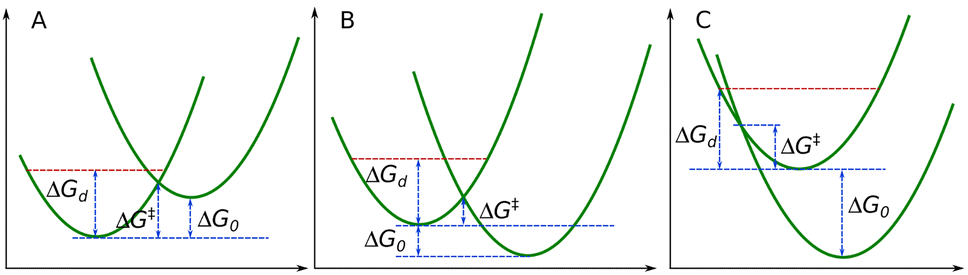Scheme 2 Free energy profiles illustrating endergonic (A) and exergonic ET processes (B) and (C) where the Marcus model predicts smaller barrier for ET (ΔG^‡) than the diffusion limit (ΔG_d, red dashed line). Under these circumstances the ET occurs in the diffusion-controlled limit within a range of reaction free energy ΔG₀.

There is a range of reaction free energies for a given λ which leads to diffusion control. The upper and lower bounds for this range of ΔG₀ values can be estimated by solving eqn (10) where ΔG^‡ is replaced with ΔG_d. Equivalently, employing eqn (8) we can describe the diffusion-controlled region using a reduction potential range: within this range the rate of electron transfer is constant (see SI, Fig. S2 for details). It is clear that diffusion control can occur for both endergonic (Scheme 2A) and exergonic (Scheme 2B and C) ETs.

The steady state established in our photocatalytic model system is due to the constant photon flow from the lamp. For a monochromatic lamp having a given effective power the volumetric photon radiation (I_p, the number of photons entering a unit volume of the system per unit time, i.e., the rate of the photon flux) can be estimated (see SI, 1.4). The rate of photon absorbance (I_a, the rate of the production of PC*) can then be estimated by the following equation obtained from the Beer–Lambert law:

I_a ≈ I_p(1 − 10^{−[small epsilon, Greek, macron][PC]l}) (11)

where [small epsilon, Greek, macron] is the mean or effective absorption coefficient of PC in the narrow frequency region emitted by the lamp and l is the path length of the light in the catalytic system (see SI, 1.5. for the derivations). Therefore, an effective rate coefficient k₁ can be derived from the following equation:

I_a = k₁[PC] (12)

i.e., by dividing I_a with the instantaneous concentration of PC. Note that k₁ depends on [PC] and thus on reaction time t. Another important approximation is using I_a in place of the true v₁. This assumes a quantum yield of unity for the population of the photoactive excited state. Note however, that we have evaluated the impact of this approximation by varying I_a through changes in the mean absorption coefficient; further discussion is provided in the Results section.

PC* participates in ET according to eqn (3), but it can also spontaneously relax to PC following first order kinetics (eqn (1), backward). The corresponding rate constant k₂ can be derived from the lifetime (τ) of the excited state: k₂ = τ⁻¹. We use a default value of 10 ns in the simulations as it is a typical value for organic photcatalysts,^1c but we also explore the effect of changing τ in a dedicated section in Results.

By following the time evolution of the concentrations, the steady-state properties (such as E_Q) can be determined for arbitrary sets of parameters (standard ground and excited state reduction potentials, absorption coefficient, lamp intensity, solvent parameters, such as λ and diffusion barrier, cage-escape yield, lifetime of the excited state). Optimizing photocatalyst selection requires a systematic study of how these parameters influence the photocatalytic performance measured by the steady-state reduction potential E_Q. Our strategy is the following: we define practically relevant ranges for the parameters, and study how the systematic variation of the parameters affects photocatalytic activity. Note that more sophisticated mathematical procedures are available to explore the effects of multiple parameters, such as dimensionality reduction methods (e.g. principal component analysis, partial least squares regression, etc.) or other methods such as response surface methodology.¹⁷ However, the results indicate that a one-by-one analysis is sufficient to understand the relevant dependencies. These findings can help to identify effective photocatalysts for given experimental conditions.

As all PCs are characterized by their ground state and excited state standard reduction potentials, we consider E_Q as the 2D function of these two quantities . Then we systematically study how the variation of other parameters affects this 2D function. Specifically, we seek the region where E_Q reaches its minimum (most negative) value, corresponding to the optimal photocatalytic performance. To that end, we define photocatalytically relevant ranges for E⁰_PC and based on the following observation: for a given quencher Q with standard reduction potential E⁰_Q, a suitable PC cannot have arbitrary E⁰_PC. The fact that PC does not spontaneously reduce Q (otherwise we would not use light for the activation) implies that ET must be very limited between PC and Q. Assuming that at most 1‰ [Q⁻] is present when PC and Q are together without light, we can derive the following expression (the derivation is given in SI, 1.6.):

E⁰_PC > E⁰_Q + 0.35 V (13)

Regarding we can identify the following constraints. For a reductant PC, oxidation of PC* is energetically more favorable than that of PC, hence . This can be further improved based on their relationship:^1c,18

where ε_0,0 is the 0-0 transition energy between the relevant excited and ground states. However, there are two common excited states: the S₁ and the T₁ states. The ground state of most organic photocatalysts is singlet so light absorption initially yields the S₁ state after ultrafast relaxation from higher singlet states. S₁ can remain the photocatalytically active state if the main relaxation pathway is fluorescence (i.e., fluorescence quantum yield near 1) with lifetime around 10 ns.^1c Such PCs are in high demand as they can offer exceptional reductive (or oxidative) power due to their large ε_0,0. Note that for PCs with S₁ lifetimes in the 1–10 ns range a relatively large quencher concentration is required to obtain reasonable reaction rates. PCs with longer-lived T₁ active states allow for lower reactant concentrations. Transition metal catalysts are the typical choice here, but benzophenone derivatives or more recently the targeted design of BODIPY dyes are also a prime example.¹⁹ Our model applies to all active states, irrespective of the nature of the PC, but the correct (S₁ or T₁) ε_0,0 energy of the photocatalyst must be specified to determine the excited state reduction potential. As we focus on absorption in the visible range, the lower and upper bounds on the reduction potential of PC* can be conveniently defined. Regarding the upper bound, a conservative estimation for ε_0,0/F is 1.0 V, i.e. ; because ε_0,0 is located at lower energy than the lowest-energy absorption observed in the spectrum. A plausible lower bound can be set by taking 4.1 eV as the higher energy limit: this sets 300 nm as the lower bound for the 0–0 transition a visible light photocatalyst can have. Hence the range we consider for the excited state reduction potential is:with these constraints, we can set the relevant regions of the reduction potentials, taking also into account the practically accessible range of the ground state reduction potentials of the photocatalysts and quenchers. (For reductive quenching the derivation can be found in the SI, 1.7.) We can also notice that the rate coefficients of all the ETs depend only on reduction potential differences, hence either E⁰_PC or E⁰_Q can be fixed and the other reduction potential as well as can be varied relative to the fixed potential. This is a useful observation because one less parameter is involved in the analysis. The conclusions are transferable to other situations where the differences in reduction potentials are the same. For example, in our analysis E⁰_Q is fixed at −0.45 V (with respect to SCE) to represent moderate oxidative power. Evidently, for another quencher with a different E⁰_Q value the photocatalytically relevant ranges of E⁰_PC and are redefined by eqn (13)–(15).

Computational details

The kinetic modelling is carried out using the COPASI microkinetic software.²⁰ The time evolution of the reactions constituting eqn (1)–(3) is followed. The initial concentration of PC and Q is 1 M. The rate of the forward reaction of eqn (1) is given by eqn (11). The backward rate, i.e., the spontaneous relaxation of the excited state of PC* (comprising various possible channels, such as fluorescence or thermal decay) is set to 1 × 10⁸ s⁻¹ but variation of this value is also tested.²¹ Rate coefficients k₃–k₆ are derived using eqn (6). The instantaneous rates are calculated by the corresponding rate equations using the instantaneous concentrations. The activation barriers are determined using eqn (10) assuming uniform λ for each step. To reach steady state we used 10⁸ s for simulation time; we note that shorter simulation time is sufficient in most cases (see SI, Fig. S3 and S4). The reaction free energies in eqn (10) are computed from the relevant standard reduction potentials using eqn (8). The default parameter values were selected either as midpoints within their feasible ranges or to reflect typical experimental conditions. Additional details of the kinetic modelling are available in the SI and in the files uploaded on github.com/acsstirling/photokinetics.

Results

The principal quantity we are interested in is the value of E_Q (the steady-state reduction potential of Q) as a function of E⁰_PC and . As we consider oxidative quenching where PC is the reducing agent, lower E_Q values indicate stronger reduction power for the PC, so we seek parameter combinations that minimize E_Q. Fig. 1 shows E_Q, as the function of E⁰_PC and when the other photocatalytic parameters (such as E⁰_Q, λ, lamp intensity, cage-effect yield, etc.) are fixed. In particular, cage-escape yield ϕ_ce is set to 1, i.e., we assume that nonproductive recombination (eqn (3b)) does not take place. The effect of ϕ_ce is presented later. The values of E_Q exhibit a very peculiar pattern: for specific values of , E_Q remains constant over a wide range of E⁰_PC as shown by the straight horizontal contour lines; and the same behavior is seen for selected E⁰_PC values, where E_Q remains constant along an interval of . The ideal PCs that yield the lowest E_Q of −0.86 V under the conditions defined by the other parameters are those featuring E⁰_PC ≈ 2.1 V and .

Fig. 1 E_Q (V) as a function of E⁰_PC and when E⁰_Q = −0.45 V. The side graphs show slices at constant values of (top) and E⁰_PC (right). The red countour lines are separated by 0.02 V. Concentration values of [Q⁻] and [PC⁺] smaller than 5 × 10⁻¹³ mol l⁻¹ were set to this threshold for generating the E_Q distribution. Other parameters were kept at the following values: ϕ_ce = 1; I_p = 0.0564 mol dm⁻³ s⁻¹; [small epsilon, Greek, macron] = 0.1 m² mol⁻¹; λ = 0.564 eV; ΔG_d = 0.166 eV; τ = 1 × 10⁸ s⁻¹.

The variation of E⁰_PC and within their respective ranges can induce huge changes (tens of orders of magnitude) in the rate constants, due to their exponential dependence on the free energy barriers as shown in Fig. 2. This is key to understanding the observed variation patterns of E_Q in Fig. 1. We first consider the relative magnitudes of the rate constants under steady-state conditions. k₁ (the effective rate constant of the production of PC*) is of order 10¹⁰ s⁻¹ (obtained from eqn (12)). The annihilation of the excited state by relaxation to the ground state is a fast process, a typical value of k₂ is 10⁸ s⁻¹.²¹ Fig. 2 displays the variation of k₃, k₄, k₅ and k₆ (see eqn (2) and (3) as the function of E⁰_PC and when E⁰_Q is set to −0.45 V. In this case k₃ and k₄ are determined solely by E⁰_PC, whereas k₅ and k₆ are determined solely by as indicated by the vertical and horizontal contours, respectively. For both k₃ and k₄ we can see an exponential decrease with increasing E⁰_PC corresponding to scenarios depicted on Schemes 1A and D, respectively. In contrast, it is seen that as becomes more negative, k₅ first increases until diffusion control and remains constant within an interval of 1.15 V; then, in the Marcus inverted region, it starts to decrease below diffusion control around −1.65 V. The same pattern is seen for k₆: as increases, it first increases reaching the diffusion rate at ; then above 0.75 V it departs from the diffusion-controlled regime within the Marcus inverted region and starts to decrease. Note that in their seminal study Rehm and Weller showed the lack of the inverted region for selected bimolecular reactions.²² Later however the existence of the inverted region for bimolecular reactions has been conclusively demonstrated.²³

Fig. 2 Calculated rate constants (mol l⁻¹ s⁻¹) of eqn (2) and (3) as the functions of E⁰_PC and when E⁰_Q = −0.45 V, I_p = 0.0564 M s⁻¹; [small epsilon, Greek, macron] = 0.1 m² mol⁻¹; λ = 0.564 eV; ΔG_d = 0.166 eV; τ = 1 × 10⁸ s⁻¹. Coloring is logarithmic. The largest values (dark red regions) are of order 10¹⁰ M⁻¹ s⁻¹, corresponding to diffusion control. It is seen that since the rate constants are obtained from eqn (9), they depend strictly on either E⁰_PC or .

A closer inspection of the rate landscape (Fig. 2) shows that in the region where lies above roughly −1 V while E⁰_PC shifts toward strongly positive values (≈+1.5 V and beyond), the backward electron-transfer pathway leading to PC* (k₆) becomes markedly more favorable than the corresponding path regenerating PC (k₄). In this domain, recombination of PC⁺ and Q⁻ can directly populate the excited state even in the absence of photoexcitation, consistent with known chemiluminescent and electrochemiluminescent mechanisms.²⁴ A classic example is the Ru(bpy)₃²⁺ system, where back electron transfer produces the emissive excited state.²⁵

Interplay between the forward and backward rates of eqn (2) and (3) governs the equilibrium ratio [Q⁻]/[Q] and thus E_Q. The specific patterns (straight contours) seen on Fig. 1 can be understood by identifying the actual source of [Q⁻] at a given pair. Horizontal contours indicate that reaction (2) has negligible role in producing and consuming Q⁻, whereas vertical contours point to the negligible role of excitation. For example, the vertical contours on the left side of Fig. 1 signal that the actual E_Q is higher than E⁰_Q (−0.28 eV when E⁰_PC = −0.1 eV and it increases as E⁰_PC increases), i.e., [Q⁻] is order of magnitudes smaller than [Q]. In this region reaction (2) is the main source of Q⁻, both the forward and backward rates (v₃ and v₄) are significantly higher than the rates of eqn (1) and (3) (see SI, Fig. S5 and S6 for the actual values). For larger values of E⁰_PC, v₃ and v₄ rapidly become very small and reaction (3) becomes the main source of Q⁻. The local maximum plateau at E_Q = −0.12 eV indicates a shift in the relative importance of reactions (2) and (3). In particular, it is crucial that v₄ diminishes significantly as this allows the accumulation of Q⁻. In contrast, around the minimum region of E_Q, Q⁻ is dominantly formed via reaction (3). In this region [Q⁻] is orders of magnitude higher than [Q] yielding E_Q potentials far more negative than E⁰_Q. In this region the largest rates are those of the photoexcitation and deexcitation, followed by the rate of the photoredox production of [Q⁻] and the backward ET in reaction (2) (see SI, Fig. S5–S7 for the plots). The other rates are orders of magnitude smaller in this region. Along the rest of the contours both the ground and excited states play equally important roles in determining E_Q.

Effect of the reorganization energy

A crucial parameter affecting the performance of a photocatalyst is the reorganization energy (λ) in the actual solvent. Reorganization energy λ can be expressed as the sum of two terms: λ = λ_i + λ_s; where λ_i arises from the structural changes of the solvated reactants to match the structure of the products at the moment the ET takes place; the other term λ_s is the energy required for the accompanying solvent rearrangements. The significance of dividing the reorganization energy into two components is that they impact photocatalytic efficiency differently: λ_i is large, when ET requires significant structural changes, such as when ET gives rise to Jahn–Teller distortion;²⁶ however this is not typical in most situations, and solvent contribution λ_s is the dominant.^13a,27,28 eqn (9) and (10) indicate complicated nonlinear relation between λ and the ET rates.²⁹ As the rates also depend on the ΔG₀ free energies of the ETs, the final E_Q is very difficult to predict in advance (see SI, Fig. S2 for illustrative plots). This dependence implies that ΔG^‡ is minimal if λ = |ΔG₀|; for either larger or smaller λ values the activation barrier increases, i.e. the rate of ET continuously decreases (note that this effect is masked in the diffusion-controlled region, see earlier discussion). As the ΔG₀-s of the ET-s depend on E⁰_PC or (see eqn (8a) and (8b)), the changes in the ET rates brought by variation in λ can be very diverse. We have performed the same simulation discussed for Fig. 1 considering a wide range of relevant λ values and determined the optimal (lowest) E_Q for each λ. The results are plotted on Fig. 3. The individual plots (analogous to that of Fig. 2) are in the SI, Fig. S8.

Fig. 3 Optimal E_Q as a function of the reorganization energy λ. The right axis indicates the corresponding concentration ratio of the reduced and oxidized form of Q. The dashed horizontal line indicates the standard reduction potential E⁰_Q of Q (−0.45 V, when [Q] = [Q⁻]). Variation of λ has been carried out with the same parameter setup as for Fig. 2. The lowest E_Q (−0.88 V) is obtained at λ = 0.58 eV. The blue line is a guide to the eye.

Fig. 3 clearly shows that large reorganization energies are detrimental to photocatalytic activity. In fact, above λ = 1.4 eV, the photocatalysts become ineffective as E_Q is above E⁰_Q (i.e., [Q⁻] < [Q]). In contrast, we can find an ideal λ where the strongest possible reductive power can be obtained under the given conditions. Looking at the underlying 2D plots for each point in Fig. 3 (see SI, Fig. S7) we can infer that as λ increases, the position of the optimal E_Q shifts toward larger values of E⁰_PC, beyond the photocatalytically relevant domain (to regions where the excitation of PC requires UV energy). It is also seen that as λ increases, the relevant domain features a larger region where their variations do not affect the steady-state E_Q value. This is related to the fact that larger λ results in broader reduction potential ranges where the rate of ET is diffusion controlled (see SI, eqn (S15)). This implies that higher λ leads to stronger leveling effects and an overall adverse impact on the catalytic efficiency of visible-light photocatalysts. Specifically, employing a solvent where λ is more than 1 eV larger than its optimal value for a given PC–Q pair, less than half of Q can be reduced under the given circumstances. For small reorganization energies the efficiency again decreases, the optimal E_Q values are less negative. This is related to the fact that for small λ values the rate constants for most pairs are smaller. It is also seen that around the optimal reorganization energies, a change of 0.5 eV in λ results in a decrease of ∼0.2 V in E_Q. This is a significant change that highlights the importance of the reorganization energy for photocatalysis. From a practical point of view, it shows that the solvent selection strategy for photocatalysis must carefully consider reorganization energy. Also note that in real-world applications the choice of the solvent affects the value of not only λ but also E⁰_PC and .

Effect of the intensity of the lamp

The effect of lamp intensity is straightforward as seen in Fig. 4. The stronger the light intensity I_p the more effective the photocatalyst is in terms of reduction power. Note that the pair that characterizes the optimal PCs (i.e., where E_Q is minimal) remains in the same region, indicating that its dependence on the light intensity is marginal (see SI, Fig. S9). The slope of the line is −39 mV, i.e. it is close to the ideal Nernstian slope (59 mV). This suggests that the observed trend is partly governed by Nernst-type behavior; however, the deviation from the ideal value points to additional kinetic and transport effects, and no simple analytical relationship could be identified. It follows that orders of magnitude change in the intensity results in fractions of eV change in the reduction potential. The model therefore suggests that lamp intensity is not the primary factor to consider for improving photocatalytic performance. In turn, only a significant loss of intensity can lead to an observable loss of steady-state performance, as far as the light setup is concerned.

Fig. 4 Optimal E_Q (V) as a function of the photon intensity of the illuminating lamp (I_p). The horizontal scale is logarithmic. The dashed blue line is the linear regression fit to the data.

Effect of the mean absorption coefficient of the PC

Another important property related to the activity of a PC is its mean absorption coefficient ([small epsilon, Greek, macron]) in the frequency region of the illuminating light. The exponential dependence of the absorbed light on [small epsilon, Greek, macron] translates to a near linear dependence of the optimal E_Q on the logarithm of [small epsilon, Greek, macron] as seen in Fig. 5 (slope is −43 mV). Similarly to the case of light intensity, if the other parameters are fixed, then changes in the optimal values are minimal when [small epsilon, Greek, macron] is varied (see Fig. S10 for the corresponding plots). Indeed, we can see that three orders of magnitude change in [small epsilon, Greek, macron] results in only a ∼0.1 V change in the optimal reduction potential.

Fig. 5 Optimal E_Q (V) as a function of the effective absorption coefficient of the PC. The horizontal scale is logarithmic. The dashed blue line is the linear regression fit to the data.

Effect of the excited state lifetime

The lifetime of the excited state of the photocatalysts (τ) is the crucial timescale defining how long the catalyst remains in its active state. For higher efficiency, this lifetime should be longer than the diffusion-controlled timescale to ensure reactive encounters. PCs with triplet active states usually satisfy this condition which is the reason why transition-metal photocatalysts are widely employed in photocatalysis.³⁰ The design of organic PCs is evidently more challenging for this reason, however, there are already several scaffolds like cyanoarene, acridinium, phenazine, etc. that offer either a longer-lived active S₁ state, access to higher lying triplets or even super reducing excited radicals.^1a Note that this does not mean that PCs with short lifetimes cannot react. To compare the timescales of diffusion and fluorescence decay, the diffusion rate constant first needs to be converted to effective first order using k_eff = k_d[Q] so it can be compared to k₂ (we can do this because [Q] ≫ [PC*]). This implies that promoting the probability of collisions by increasing the initial concentrations of the reactants (preferably Q), PCs with short lifetimes can also be effective. Also note that while τ has an important limiting effect, this parameter alone is not a reliable predictor of photocatalytic activity.³¹

Our simulations indicate that τ and equivalently the rate constant of deexcitation of PC* has again a straightforward effect on the strongest attainable reduction potential when the other parameters are fixed: the longer the lifetime (i.e., the smaller the corresponding annihilation rate constant k₂) the deeper the optimal potential is as shown by Fig. 6 (full plots are in SI, Fig. S11). Indeed, longer excited state lifetimes yield larger PC* concentrations which in turn result in concentration increase for Q⁻. The linearity on the logarithmic k₂ scale (slope is 36 mV) is again related to the logarithmic dependence of the reduction potential on concentrations via the Nernst equation.

Fig. 6 Optimal E_Q (V) as a function of k₂ (i.e., the inverse of the lifetime (τ) of PC*) when the rate of diffusion is 1 × 10¹⁰ l mol⁻¹ s⁻¹. The horizontal scale is logarithmic. The dashed blue line is the linear regression fit to the data.

Effect of the diffusion-controlled rate

An important factor that influences the optimal reduction potential E_Q is the maximal possible rate of the reaction steps. For the ET steps this rate is the diffusion-controlled rate. The rate constant of diffusion (k_D) can be given in typical situations under reasonable assumptions (such as neutral reactants and similar sizes; see ref. 16): k_D = 8k_BT/3η, where η is the viscosity of the solvent. Clearly, as viscosities do not have orders of magnitude differences for typical solvents, the diffusion limit predicted by the above equation varies in a small range. However, when long range interactions are important, such as when charged species are involved, then the previous formula is not valid and k_D can change significantly.^16,32 We therefore set the range of the diffusion-controlled rate constant considered here to span 7 orders of magnitude (from 1 × 10⁴ to 1 × 10¹¹ l mol⁻¹ s⁻¹) and determined the optimal E_Q, when the other parameters were unchanged. We can see in Fig. 7 (full plots are in SI, Fig. S12) that departure from the typical diffusion-controlled limit (∼10¹⁰ l mol⁻¹ s⁻¹) starts to influence the performance below the threshold of 10⁸ l mol⁻¹ s⁻¹ (with a slope of −55 mV). From this value onwards the diffusion-controlled rate is smaller than the deexcitation rate hence the formation of Q⁻ is suppressed. Indeed, k₂ can be decreased to compensate for the effect of the decreasing diffusion rate (see SI, S13). This is in accord with our observations that a longer lifetime for PC* results in better E_Q (i.e. more negative; see Fig. 6).

Fig. 7 Optimal E_Q (V) as a function of the diffusion-controlled rate constant when k₂ = 10⁸ s⁻¹. The horizontal scale is logarithmic. The blue line is drawn to guide the eye.

Effect of cage-escape yield ϕ_ce

We have performed kinetic simulations with various ϕ_ce values. Fig. 8 shows how the optimal E_Q obtained under steady-state conditions depends on ϕ_ce. Clearly, as shown in Fig. 8 the magnitude of E_Q decreases with decreasing ϕ_ce exhibiting a linear dependence when plotted as a function of log(ϕ_ce). We can also see that under steady-state conditions, the photocatalytic process approaches the optimal performance even for smaller ϕ_ce values.

Fig. 8 Optimal E_Q (V) as a function of the cage-effect yield under steady-state conditions. The linear regression line is dashed blue. The horizontal scale is logarithmic.

Discussion

Kinetic modelling offers significant utility in catalysis;³³ it can help understand the effect of the various parameters that define a photocatalytic setup and it can identify the optimal photocatalysts for that particular setup. As an example, Fig. 9 displays the distribution of selected photocatalysts as a function of their E⁰_PC and values projected onto the computed E_Q surface. Note that displaying a set of photocatalysts on the same plot assumes identical reorganization energies, cage-effect yields, excited-state lifetimes, and absorption properties, all measured in the solvent associated with the plot. Still, the distribution in the figure clearly shows that the different photocatalysts form well-defined groups based on their core structures.

Fig. 9 Distribution of organic PCs from the database of ref. 18 as a function of their standard ground state (E⁰_PC) and excited state reduction potentials relevant for oxidative quenching projected onto the computed E_Q surface. Colors indicate the molecular scaffolds of the photocatalysts. Experimental data are taken from ref. 18.

The contour patterns seen for specific regions in Fig. 1 and the distribution of the photocatalysts represented by the colored circles on Fig. 9 give pragmatic hints for achieving higher photocatalytic efficiencies. First, it is quite clear that the compounds with the same scaffold form well-defined clusters on the plot indicating that the role of the side chains is more about fine-tuning. (Note, that independent tuning of E⁰_PC and in practice may not be possible, as both are inherently linked to the molecular structure.) Horizontal contours imply that strategic modifications of a PC affect E_Q only via the induced variations in its but changes in E⁰_PC has no effect along the horizontal contours. Vertical contours imply the same perspective but swapping the role of and E⁰_PC. This, in turn, signifies design flexibility, as the straight vertical and horizontal contours indicate that in those regions, variations in the corresponding reduction potential do not affect the photocatalytic potential. In particular, the vertical contour pattern at the region 1.0 V ≤ E⁰_PC ≤ 1.6 V suggests a counterintuitive strategy to improve the efficiency of a PC by increasing its ground state reduction potential: indeed, this strategy exploits the fact that at very large E⁰_PC values the increasing exergonicity of the backward ET of reaction (2) shifts its rate to the Marcus inverted region and it becomes less effective to oxidize Q⁻ back to Q. Overall, Fig. 9 shows that both the standard ground state and the excited state potential of a photocatalysts have to be taken into account for optimizing the photocatalytic efficiency.

The selection of solvent plays a critical role,⁸ as it impacts several key parameters – such as excitation energies, reduction potentials, reorganization energy, diffusion limit, cage-escape yield, excitation state lifetime – that, in turn, influence the efficiency of photocatalysis. We now take a closer look at each relevant parameter separately. For the model to be applicable, the reduction potentials must be determined in the selected solvent, as solvents with different polarity stabilize the oxidized and reduced forms differently.^8b Similarly, the diffusion limit that determines the maximum achievable reaction rate can be very different in typical solvents used for photocatalytic reactions, but as we have shown, this effect is limited. We note that in traditional catalysis mass transfer limitations must be carefully considered.³⁴ Our kinetic model assumes ideal mixing for proper diffusion. Regarding the lifetime of the excited state of the photocatalyst, it has been found that polar media can enhance it,³⁵ but this effect is often limited.³⁶ Another key parameter affected by the solvent is the reorganization energy that is comprised of two components: the outer-sphere λ_s reorganization energy of the solvent and the inner-sphere λ_i reorganization energy of the reactants. According to classical solvation models, the solvent reorganization energy for the electron-transfer reaction is expected to decrease with decreasing solvent polarity.¹² However, nonpolar solvents often exhibit significant reorganization energies, challenging earlier assumptions.³⁷ In fact, it can reach 0.3 eV in typical nonpolar solvents.^37d Inner sphere reorganization energies can also vary significantly depending on the oxidant and reductant³⁸ but specific ligand-sphere designs can effectively decrease them³⁹ by minimizing the extent of geometrical stabilization required during electronic relaxation upon ET. Note that the reorganization energy can be readily calculated using quantum chemical methods with implicit solvation models, based on Marcus’ theory.⁴⁰ Altogether, the solvent is a pivotal factor in photocatalytic systems, because it influences key electron-transfer parameters, i.e., it affects both the mechanism and the efficiency.

In the following, we discuss how the cage escape yield (ϕ_ce), which is the main descriptor of the cage effect,^13a,b can be derived within the framework of our model. The cage-escape yield is independent of how the cage is formed; it describes the competition between charge recombination and diffusive escape processes. These main substeps are highlighted using the relevant parts of the simple Marcus parabolas shown in Fig. 10 and the energy profile in Fig. 11.

Fig. 10 Marcus parabolas depicting the ET-s occurring between PC and Q as well as between PC* and Q, indicating the energy penalties required by the cage effect, shown somewhat overstated for clarity. Dashed lines indicate the original parabolas. Curly brackets indicate solvated species. The excited state parabola is lighter to indicate the limited role of the excitation state in the cage-effect.

Fig. 11 Schematic free energy profiles representing the two competing processes in a solvent cage shortly after the ET from PC* occurred. Curly brackets indicate solvated species. The new free energy quantities shown in the figure are as follows: ΔG^‡_cr is the barrier for charge recombination, ΔG^‡_ce is the barrier for cage-escape, whereas ΔΔG^‡ is the difference between the former two activation energies. The barrier of the formation of {PC + Q} is not shown for simplicity (cf. Fig. 10). Note that ΔG^‡ denotes here the barrier for ET from the ground state PC to Q.

The cage-escape yield (ϕ_ce) characterizes the efficiency of the separation of the target PC⁺ and Q⁻ ion pair as shown by eqn (6). For the purpose of kinetic modeling, simple algebraic manipulation yields an expression that allows cage-escape to be characterized by experimentally available quantities:

Here we assume the validity of eqn (9) (Eyring formula) for the rate constants. As Fig. 11 indicates: ΔΔG^‡ = ΔG^‡ − ΔG_d − ΔG₀. Using eqn (10) it can be further transformed into the following expression: ΔΔG^‡ = (λ + ΔG₀)²/4λ − ΔG_d − ΔG₀; i.e., ϕ_ce is a nonlinear function of the properties of PC, Q and the solvent. Substituting eqn (8) into this expression reveals the link between cage-escape efficiency and the standard reduction potential difference of PC and Q: ΔΔG^‡ = (λ − zFΔE₀)²/4λ − ΔG_d + zFΔE₀. Eqn (17) shows the final formula for cage-escape yield:

An important observation is that ϕ_ce does not depend on 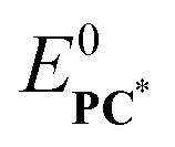, only on the ground state reduction potentials E⁰_PC and E⁰_Q. It is quite remarkable, that ϕ_ce can be predicted for a given PC–Q pair from eqn (17) within the assumptions of the kinetic framework introduced above, if reorganization energy λ is available. Given the importance of ΔΔG^‡, Fig. 12 shows its distribution as a function of E⁰_PC–E⁰_Q and ΔG_d.

Fig. 12 Distribution of ΔΔG^‡ (eV) as a function of E⁰_PC–E⁰_Q and ΔG_d. λ = 0.564 eV.

Fig. 12 provides several insights. ΔΔG^‡ is mostly positive, becoming negative only in the upper left region of the plot where the ΔE₀ values are very small and diffusion barriers are large. In typical photocatalytic processes ΔE₀ exceeds 0.8–1 eV,⁴¹ therefore negative ΔΔG^‡ values are expected only in viscous solvents that exhibit high diffusion barriers. From a reaction kinetics perspective, a negative ΔΔG^‡ indicates that the activation barrier for the reverse ET reaction (eqn (2)) is higher than that predicted by Marcus theory. Conversely, a positive ΔΔG^‡ indicates that the simple Marcus model is valid for the reverse ET process. In fact, this is the situation depicted by both Fig. 10 and 11. Chemical intuition and also formal analysis indicate that the net rate of a reversible reaction remains unchanged if it is replaced by a sequence of lower-barrier substeps, provided all newly introduced intermediates are less stable than the original reactant and product states (preequilibrium assumption).^42,43 This implies that the intermediate states do not accumulate and remain kinetically inaccessible on the timescale of the overall process. Therefore, as long as ΔΔG^‡ is positive and the assumptions of the Marcus model hold, our model can deliver its central quantity E_Q without explicitly including the cage-bound ion pair in the kinetic equations. Despite treating the cage effect at an effective level, the model still captures essential features of the cage effect and allows us to extract mechanistic insight, as shown below.

Having justified the approach taken to account for the cage effect, we now show that the model can reproduce experimental observations including steady-state as well as transient measurements. As a benchmark, we selected the [Ru(bpy)₃]²⁺–tri-p-tolylamine (TTA) system and collected experimental data from ref. 13b and 28. We use our kinetic model to reproduce the experimental kinetic measurements associated with the photoinduced reaction of this photoredox system. Note that the underlying process is reductive quenching, but the same formalism can be applied. Using COPASI, we fit the key kinetic parameters (ϕ_ce, τ, k₄, k₅), along with additional experimental parameters (such as the initial concentration of [Ru(bpy)₃]²⁺ and the laser pulse duration) required to reproduce the measurement conditions. The absorption coefficients ε were taken from the literature. The parameters were determined using a global fit to obtain a consistent description of the spectroscopic data published in ref. 13b and 28, simultaneously considering measurements at different laser intensities and quencher concentrations (for details see SI, chapter 4). Given that ground-state electron transfer and excited-state regeneration via back electron transfer are expected to be negligible under the present conditions, and that the corresponding rate constants cannot be reliably determined from the available experimental data, we employ a simplified version of the model and set k₃ and k₆ to zero. The results of the fitting procedure are summarized in Fig. 13 and Table 1.

Fig. 13 Reproduction of spectroscopic measurements of the photoinduced reaction [Ru(bpy)₃]²⁺* + TTA = [Ru(bpy)₃]⁺ + TTA⁺. (A) Excited state absorbance (at 450 nm) decay of [Ru(bpy)₃]²⁺* produced by different laser powers. (B) Photoluminescence quenching of [Ru(bpy)₃]²⁺* in the presence of increasing amounts of TTA in CH₃CN. (C) Experimental and fitted Stern–Volmer plots. (D) Simulated transient concentrations of the different Ru species. Note that for this plot the horizontal scale is logarithmic. The length of the laser-pulse is 25 ns (also obtained from fitting). Its duration is indicated by the vertical dashed grey line.

Table 1 Most important kinetic parameters for the photochemical reaction of [Ru(bpy)₃]²⁺* + TTA. Reported values are best-fit parameters; the accompanying values represent standard deviations as obtained from the parameter estimation procedure in COPASI. Note that the reported parameter uncertainties do not fully address parameter identifiability or covariance issues inherent to multiparameter kinetic fitting

Parameter	Fitted value	Experiment^a
a Experimental values are from ref. 13b and 28.b Experimental value is not available.
ϕce	0.96 ± 0.01	0.84
τ (ns)	880 ± 8	890
c0([Ru(bpy)3]^2+) (µM)	7.4 ± 0.1	—^b
k4 (M^−1 s^−1)	6.15 × 10^10 ± 7 × 10^8	—^b
k5 (M^−1 s^−1)	5.23 × 10^8 ± 9 × 10^6	6.4 × 10^8; 8.5 × 10^8

---

Fig. 13(A)–(C) display the results of kinetic parameter fitting to experimental measurements. We can see that the fitted datapoints closely match the experimental curves, demonstrating that the fitted parameters reliably capture the observations. This also supports that the kinetic model captures the key steps and species, and can accurately describe the behavior of the photocatalytic system even without explicitly including the cage-bound ion pair. Table 1 lists the fitted parameters together with values derived directly from experiment. Fig. 13D displays the simulated concentration changes of the Ru species. The concentration of [Ru(bpy)₃]²⁺* increases until 25 ns (i.e., during the excitation time), and roughly 65% of the photocatalyst molecules become excited. Based on the peak maxima, 67% of [Ru(bpy)₃]²⁺* transforms to [Ru(bpy)₃]⁺, which relaxes back to [Ru(bpy)₃]²⁺ on the ms timescale. It is seen that the back electron transfer is significant during the formation of the oxidized quencher, which explains the difference between the globally fitted cage escape yield and the experimentally determined value (0.96 vs. 0.84).

This kinetic analysis provides a unified mechanistic interpretation of all transient spectroscopic data for the Ru complex. An important advantage of the model is its explicit treatment of excited-state formation: instead of assuming instantaneous population of [Ru(bpy)₃]²⁺*, it accounts for the finite laser-pulse duration by integrating the absorbed photon flux. This yields a physically accurate estimate of the initial [Ru(bpy)₃]²⁺* concentration, avoids systematic errors inherent in delta-function excitation approximations and improves the reliability of all downstream kinetic parameters. The model also enables quantitative determination of back electron transfer, a process that overlaps with several microscopic pathways in the experiment, making it difficult to measure directly. Hence, the model can provide a good estimate of the fraction of the TTA⁺ lost prior to a potential photocatalytic turnover. In summary, the kinetic modeling furnishes mutually consistent and physically meaningful rate constants, while offering predictive capability beyond what can be inferred from experiment alone, thereby enabling a more complete mechanistic understanding of the Ru-based photoredox cycle.

A crucial issue for our kinetic model is to use reliable values for those parameters which are not fitted to experiment.^8b These parameters can be taken from measurements or can be derived from analogous systems. Temperature dependent cyclic voltammetry can yield reduction potentials and reorganization energies.⁴⁴ The lifetime of a PC* can be determined by time-resolved spectroscopic methods.³ Optical measurements provide the Beer–Lambert coefficients. The technical details of the illumination setup can be used for determining the light intensity to input into the kinetic model. Computational chemistry can be a complementary source of key parameters and its integration with kinetic modeling often provides a powerful strategy for preliminary screening.³³

Conclusions

We have presented a kinetic model to assess the dependence of the performance of photocatalysts on several, photocatalytically relevant parameters including the ground and excited state reduction potentials of the photocatalysts and the quencher (or substrate), reorganization energy, excitation properties of the photocatalysts and other parameters. In addition, we have also highlighted its capability to extract kinetic parameters by fitting the simulations to experimental measurements. The model comprises the kinetics of the following processes: photoexcitation and subsequent decay, electron transfer (ET) between the photocatalyst (in both ground and excited states) and the quencher with explicit treatment of solvent-cage escape, and the unproductive quenching of the excited-state photocatalyst. We use steady-state reduction potential E_Q as an effective measure of photocatalytic performance. To demonstrate the utility of the model, we have systematically mapped the dependence of E_Q on the ground and excited state reduction potentials of the photocatalyst within their catalytically relevant ranges while keeping the remaining parameters at fixed values selected to reflect typical photocatalytic conditions. The plot of can be effectively used to identify the directions in which the ground and excited state reduction potentials can be tuned to improve photocatalytic efficiency. To demonstrate this, we have presented an example that employs photocatalysts commonly used in practice. Our analysis reveals that the dependence of E_Q on the reduction potentials is far from trivial: it is critically shaped by whether each electron-transfer step occurs in the Marcus normal or inverted region. This further suggests that the performance of a photocatalyst cannot be reliably assessed using only one parameter (e.g., only the excited state reduction potential, or the free energy of an ET). It is also clear that, of all the parameters considered in the model, only the reorganization energy affects the photocatalytic performance in a non-intuitive way. The model was also applied to a set of known photocatalysts, providing a practical demonstration of how it can assist in evaluating and comparing real systems. We have also presented an example where the model performance has been tested by fitting crucial kinetic parameters to transient and stationary measurements, and predicting other key experimental observables, as well as accessing information that was not directly available from the experiments. The model can also be used to predict reduction potential combinations to obtain chemiluminescence. The kinetic model presented here can be easily modified or extended with additional reaction steps as it is available freely on Github. It can be used for a rapid qualitative assessment of photocatalytic performance or for systematic exploration of how key parameters influence new photocatalytic strategies and reactivities.

In cases where a specific quencher is targeted, optimal photocatalyst can be identified by considering multiple parameters simultaneously, which the model integrates in a unified framework. Beyond catalyst selection, the model can also support the optimization of experimental setups, such as the choice of solvent, light intensity, or reactant concentrations. Furthermore, by fitting the model to experimental data, it may help interpret measurements or estimate parameters that are otherwise difficult to access. The steady-state reduction potential E_Q introduced here thus acts as a comprehensive descriptor of photocatalytic efficiency, suitable for rational design of new photocatalytic systems. We also note that the actual kinetic model can be straightforwardly extended to heterogeneous photocatalysis.

Author contributions

The manuscript was written through contributions of all authors. All authors have given approval to the final version of the manuscript.

Conflicts of interest

The authors declare no competing financial or non-financial interests.

Data availability

Supplementary information is available. See DOI: https://doi.org/10.1039/d6cp00976j.

The supporting data (additional derivations, discussions, and plots of E_Q as a function of systematic changes of parameters, Fig. S1–S13) have been provided as part of the supplementary information (SI). Simulation files are uploaded on github.com/acsstirling/photokinetics.

Acknowledgements

We acknowledge useful discussion with Prof. G. Lente. This work was supported by the National Research, Development and Innovation Office of Hungary (NKFI, Grant No. K132236).

References

1. (a) M. V. Bobo, J. J. Kuchta and A. K. Vannucci, Org. Biomol. Chem., 2021, 19, 4816–4834; (b) E. D. Talbott, N. L. Burnett and J. R. Swierk, Chem. Phys. Rev., 2023, 4, 031312; (c) N. A. Romero and D. A. Nicewicz, Chem. Rev., 2016, 116, 10075–10166; (d) N. Holmberg-Douglas and D. A. Nicewicz, Chem. Rev., 2021, 122, 1925–2016.
2. (a) N. Kandoth, J. Pérez Hernández, E. Palomares and J. Lloret-Fillol, Sustainable Energy Fuels, 2021, 5, 638–665; (b) A. A. Lee and J. R. Swierk, J. Am. Chem. Soc., 2024, 146, 34900–34908; (c) V. M. Huxter, J. Phys. Chem. Lett., 2024, 15, 7945–7953; (d) C. Wang and A. Malinoski, J. Chem. Phys., 2022, 157, 160901; (e) W. B. Swords, S. J. Chapman, H. Hofstetter, A. L. Dunn and T. P. Yoon, J. Org. Chem., 2022, 87, 11776–11782; (f) N. A. Till, S. Oh, D. W. C. MacMillan and M. J. Bird, J. Am. Chem. Soc., 2021, 143, 9332–9337; (g) B. G. Stevenson, E. H. Spielvogel, E. A. Loiaconi, V. M. Wambua, R. V. Nakhamiyayev and J. R. Swierk, J. Am. Chem. Soc., 2021, 143, 8878–8885; (h) N. Hosokawa, K. Ozawa, K. Koike, Y. Tamaki and O. Ishitani, Chem. Sci., 2025, 16, 4279–4289; (i) A. Aydogan, R. E. Bangle, S. De Kreijger, J. C. Dickenson, M. L. Singleton, E. Cauët, A. Cadranel, G. J. Meyer, B. Elias, R. N. Sampaio and L. Troian-Gautier, Catal. Sci. Technol., 2021, 11, 8037–8051; (j) N. W. Rosemann, P. Chábera, O. Prakash, S. Kaufhold, K. Wärnmark, A. Yartsev and P. Persson, J. Am. Chem. Soc., 2020, 142, 8565–8569.
3. (a) D. M. Arias-Rotondo and J. K. McCusker, Chem. Soc. Rev., 2016, 45, 5803–5820; (b) J. Zhang, B. Zhu, L. Zhang and J. Yu, Chem. Commun., 2023, 59, 688–699; (c) S. De Kreijger, M. Gillard, B. Elias and L. Troian-Gautier, ChemCatChem, 2023, 16, e202301100; (d) W. B. Swords and T. P. Yoon, Photochemistry, Royal Society of Chemistry, Cambridge, 2022, vol. 49, pp. 428–457.
4. (a) P. McDonagh, N. Skillen, P. K. J. Robertson and D. McCrudden, Curr. Opin. Electrochem., 2024, 47, 101570; (b) P. Enders, M. Májek, C. M. Lam, R. D. Little and R. Francke, ChemCatChem, 2022, 15, e202200830.
5. (a) D. Griller and K. U. Ingold, Acc. Chem. Res., 1980, 13, 317–323; (b) A. Luridiana, D. Mazzarella, L. Capaldo, J. A. Rincón, P. García-Losada, C. Mateos, M. O. Frederick, M. Nuño, W. Jan Buma and T. Noël, ACS Catal., 2022, 12, 11216–11225; (c) N. G. W. Cowper, C. P. Chernowsky, O. P. Williams and Z. K. Wickens, J. Am. Chem. Soc., 2020, 142, 2093–2099; (d) C. K. Prier and D. W. C. MacMillan, Chem. Sci., 2014, 5, 4173–4178.
6. (a) P. J. H. Williams, G. A. Boustead, D. E. Heard, P. W. Seakins, A. R. Rickard and V. Chechik, J. Am. Chem. Soc., 2022, 144, 15969–15976; (b) S. J. Horsewill, G. Hierlmeier, Z. Farasat, J. P. Barham and D. J. Scott, ACS Catal., 2023, 13, 9392–9403.
7. N. Hölter, N. H. Rendel, L. Spierling, A. Kwiatkowski, R. Kleinmans, C. G. Daniliuc, O. S. Wenger and F. Glorius, J. Am. Chem. Soc., 2025, 147, 12908–12916.
8. (a) T. Noël and E. Zysman-Colman, Chem Catal., 2022, 2, 468–476; (b) S. B. Beil, S. Bonnet, C. Casadevall, R. J. Detz, F. Eisenreich, S. D. Glover, C. Kerzig, L. Næsborg, S. Pullen, G. Storch, N. Wei and C. Zeymer, JACS Au, 2024, 4, 2746–2766; (c) M. A. Bryden, F. Millward, O. S. Lee, L. Cork, M. C. Gather, A. Steffen and E. Zysman-Colman, Chem. Sci., 2024, 15, 3741–3757.
9. (a) R. J. Rama, A. Nova and M. C. Nicasio, ChemCatChem, 2024, 16, e202400224; (b) A. K. Sharma and F. Maseras, Inorg. Chem., 2024, 63, 13801–13806; (c) T. Žibert, B. Likozar and M. Huš, Small Struct., 2025, 6, 2500221.
10. F. Strieth-Kalthoff, C. Henkel, M. Teders, A. Kahnt, W. Knolle, A. Gómez-Suárez, K. Dirian, W. Alex, K. Bergander, C. G. Daniliuc, B. Abel, D. M. Guldi and F. Glorius, Chem, 2019, 5, 2183–2194; A. J. Rieth, M. I. Gonzalez, B. Kudisch, M. Nava and D. G. Nocera, J. Am. Chem. Soc., 2021, 143, 14352–14359; N. Baris, M. Dračínský, J. Tarábek, J. Filgas, P. Slavíček, L. Ludvíková, S. Boháčová, T. Slanina, B. Klepetářová and P. Beier, Angew. Chem., Int. Ed., 2023, 63, e202315162.
11. A. Bhattacherjee, M. Sneha, L. Lewis-Borrell, O. Tau, I. P. Clark and A. J. Orr-Ewing, Nat. Commun., 2019, 10, 5152.
12. (a) R. A. Marcus, Annu. Rev. Phys. Chem., 1964, 15, 155–196; (b) R. A. Marcus, Angew. Chem., Int. Ed. Engl., 1993, 32, 1111–1121; (c) R. A. Marcus and N. Sutin, Biochim. Biophys. Acta, Rev. Bioenerg., 1985, 811, 265–322.
13. (a) M. J. Goodwin, J. C. Dickenson, A. Ripak, A. M. Deetz, J. S. McCarthy, G. J. Meyer and L. Troian-Gautier, Chem. Rev., 2024, 124, 7379–7464; (b) A. Ripak, S. De Kreijger, B. Elias and L. Troian-Gautier, STAR Protoc., 2023, 4, 102312; (c) S. De Kreijger, F. Glaser and L. Troian-Gautier, Chem Catal., 2024, 4, 101110; (d) A. Ripak, S. De Kreijger, R. N. Sampaio, C. A. Vincent, É. Cauët, I. Jabin, U. K. Tambar, B. Elias and L. Troian-Gautier, Chem Catal., 2023, 3, 100490; (e) J. Olmsted III and T. J. Meyer, J. Phys. Chem., 1987, 91, 1649–1655; (f) E. Rabinowitch and W. C. Wood, Trans. Faraday Soc., 1936, 32, 1381; (g) S. DiLuzio, T. U. Connell, V. Mdluli, J. F. Kowalewski and S. Bernhard, J. Am. Chem. Soc., 2022, 144, 1431–1444; (h) F. Draper, S. DiLuzio, H. J. Sayre, L. N. Pham, M. L. Coote, E. H. Doeven, P. S. Francis and T. U. Connell, J. Am. Chem. Soc., 2024, 146, 26830–26843; (i) C. Wang, H. Li, T. H. Bürgin and O. S. Wenger, Nat. Chem., 2024, 16, 1151–1159; (j) A. Y. Chan, A. Ghosh, J. T. Yarranton, J. Twilton, J. Jin, D. M. Arias-Rotondo, H. A. Sakai, J. K. McCusker and D. W. C. MacMillan, Science, 2023, 382, 191–197; (k) D. Koyama, H. J. A. Dale and A. J. Orr-Ewing, J. Am. Chem. Soc., 2018, 140, 1285–1293.
14. J. Z. Bloh, Front. Chem., 2019, 7, 128.
15. (a) X. L. Soto and J. R. Swierk, ACS Omega, 2022, 7, 25532–25536; (b) J. R. Swierk, Org. Process Res. Dev., 2023, 27, 1411–1419.
16. B. Peters, Reaction Rate Theory and Rare Events, Elsevier Science, 2017.
17. M. A. Bezerra, R. E. Santelli, E. P. Oliveira, L. S. Villar and L. A. Escaleira, Talanta, 2008, 76, 965–977.
18. P. P. Fehér, Á. Madarász and A. Stirling, J. Chem. Theory Comput., 2023, 19, 4125–4135.
19. (a) Z. Wang, A. Toffoletti, Y. Hou, J. Zhao, A. Barbon and B. Dick, Chem. Sci., 2021, 12, 2829–2840; (b) X. Zhang, A. A. Sukhanov, X. Liu, M. Taddei, J. Zhao, A. Harriman, V. K. Voronkova, Y. Wan, B. Dick and M. Di Donato, Chem. Sci., 2023, 14, 5014–5027.
20. S. Hoops, S. Sahle, R. Gauges, C. Lee, J. Pahle, N. Simus, M. Singhal, L. Xu, P. Mendes and U. Kummer, Bioinformatics, 2006, 22, 3067–3074.
21. M. Y. Berezin and S. Achilefu, Chem. Rev., 2010, 110, 2641–2684.
22. D. Rehm and A. Weller, Isr. J. Chem., 1970, 8, 259–271.
23. (a) S. Fukuzumi, K. Ohkubo, H. Imahori and D. M. Guldi, Chem. – Eur. J., 2003, 9, 1585–1593; (b) M. Murakami, K. Ohkubo and S. Fukuzumi, Chem. – Eur. J., 2010, 16, 7820–7832; (c) N. Takeda and J. R. Miller, J. Am. Chem. Soc., 2020, 142, 17997–18004.
24. M. M. Richter, Chem. Rev., 2004, 104, 3003–3036.
25. N. E. Tokel and A. J. Bard, J. Am. Chem. Soc., 1972, 94, 2862–2863.
26. (a) K. M. Rosso and J. R. Rustad, J. Phys. Chem. A, 2000, 104, 6718–6725; (b) E. J. Piechota and G. J. Meyer, J. Chem. Educ., 2019, 96, 2450–2466.
27. (a) D. Moia, V. Vaissier, I. López-Duarte, T. Torres, M. K. Nazeeruddin, B. C. O’Regan, J. Nelson and P. R. F. Barnes, Chem. Sci., 2014, 5, 281–290; (b) M. Kuss-Petermann and O. S. Wenger, Chimia, 2016, 70, 177–181.
28. A. Ripak, A. K. Vega Salgado, D. Valverde, S. Cristofaro, A. de Gary, Y. Olivier, B. Elias and L. Troian-Gautier, J. Am. Chem. Soc., 2024, 146, 22818–22828.
29. T. P. Silverstein, J. Chem. Educ., 2012, 89, 1159–1167.
30. (a) C. K. Prier, D. A. Rankic and D. W. C. MacMillan, Chem. Rev., 2013, 113, 5322–5363; (b) S. DiLuzio, V. Mdluli, T. U. Connell, J. Lewis, V. VanBenschoten and S. Bernhard, J. Am. Chem. Soc., 2021, 143, 1179–1194.
31. J. R. Ochola and M. O. Wolf, Org. Biomol. Chem., 2016, 14, 9088–9092.
32. G. Lente, Deterministic Kinetics in Chemistry and Systems Biology, Springer, Cham, Switzerland, 2015.
33. (a) M. Besora and F. Maseras, Wiley Interdiscip. Rev.: Comput. Mol. Sci., 2018, 8, e1372; (b) A. H. Motagamwala and J. A. Dumesic, Chem. Rev., 2020, 121, 1049–1076.
34. U. Caudillo-Flores, M. J. Muñoz-Batista, M. Fernández-García and A. Kubacka, Catal. Rev., 2022, 66, 531–585.
35. S. Xie, L. Ma, T.-F. Xiao, J. Zhang, J. Kong, Z. Kuang, M. Zhou, G.-Q. Xu, Y. Li and A. Xia, J. Phys. Chem. B, 2023, 127, 9813–9821.
36. J. V. Caspar and T. J. Meyer, J. Am. Chem. Soc., 1983, 105, 5583–5590.
37. (a) R. A. Holroyd and J. R. Miller, J. Phys. Chem. B, 2019, 123, 9206–9211; (b) C.-H. Yang, C.-I. Wang, Y.-S. Wang and C.-P. Hsu, J. Chem. Theory Comput., 2024, 20, 6981–6991; (c) P. Chen and T. J. Meyer, Chem. Rev., 1998, 98, 1439–1478; (d) D. V. Matyushov, Phys. Chem. Chem. Phys., 2020, 22, 10653–10665.
38. (a) Significant inner-sphere reorganization energies are predicted: K. M. Rosso and J. R. Rustad, J. Phys. Chem. A, 2000, 104, 6718–6725; (b) Small inner-sphere reorganization energies are predicted: X. Amashukeli, N. E. Gruhn, D. L. Lichtenberger, J. R. Winkler and H. B. Gray, J. Am. Chem. Soc., 2004, 126, 15566–15571.
39. S. Chattopadhyay, M. Mukherjee, B. Kandemir, S. E. J. Bowman, K. L. Bren and A. Dey, Chem. Sci., 2021, 12, 11894–11913.
40. (a) K. Sakanoue, M. Motoda, M. Sugimoto and S. Sakaki, J. Phys. Chem. A, 1999, 103, 5551–5556; (b) V. Vaissier, P. Barnes, J. Kirkpatrick and J. Nelson, Phys. Chem. Chem. Phys., 2013, 15, 4804; (c) D. Moia, V. Vaissier, I. López-Duarte, T. Torres, M. K. Nazeeruddin, B. C. O’Regan, J. Nelson and P. R. F. Barnes, Chem. Sci., 2014, 5, 281–290; (d) A. de Aguirre, I. Funes-Ardoiz and F. Maseras, Angew. Chem., Int. Ed., 2019, 58, 3898–3902.
41. See SI, Table S1 collecting representative examples of such PC–Q pairs.
42. E. Feliu and C. Wiuf, J. Math. Biol., 2013, 67, 1571–1597.
43. S. Kozuch and J. M. L. Martin, ChemPhysChem, 2011, 12, 1413–1418.
44. (a) C. Costentin, C. Louault, M. Robert and J.-M. Savéant, Phys. Chem. Chem. Phys., 2012, 14, 1581–1584; (b) S. Chattopadhyay, M. Mukherjee, B. Kandemir, S. E. J. Bowman, K. L. Bren and A. Dey, Chem. Sci., 2021, 12, 11894–11913.

---