Enhancing energy transport utilising permanent molecular dipoles
Received
23rd October 2025
, Accepted 15th December 2025
First published on 17th December 2025
Abstract
We study exciton energy transfer along a molecular chain while accounting for the effects of permanent dipoles induced by charge displacements in the molecular orbitals. These effects are typically neglected as they do not arise in conventional atomic quantum optics; however, they can play an important role in molecular systems. We further demonstrate how permanent dipoles can preferentially arrange energy eigenstates to support excitation transport, such as by creating energetic barriers and adding structure to the eigenspectrum. Putting all this together, we show how permanent dipoles can enhance the ability of the molecular chain to support excitation transport across a range of environmental and system configurations.
1 Introduction
Energy transport is a fundamental process in physics, essential for numerous technological applications and biochemical reactions.1 Of particular interest are nanoscale transport mechanisms, where classical and quantum-mechanical descriptions overlap. Key examples include molecular wires that can support the fast transport of electronic excitations,2–5 as well as early-stage photosynthesis, where solar energy is captured, transported, and stored as chemical energy,6,7 and artificial photovoltaic devices.8 The role of quantum coherence in enhancing natural photosynthetic efficiency remains debated.9–13 Still, its benefits in artificial systems have been established.14–25 These insights motivate further exploration of quantum interference effects in nanoscale energy transport. In many cases, excitons—electron–hole pair quasiparticles—are the primary energy carriers. However, exciton recombination, which leads to energy loss, limits efficiency in organic photovoltaic devices by affecting exciton diffusion lengths.1,26,27 The two main loss channels are nonradiative recombination, where energy dissipates as heat through phonon emission,28 and radiative recombination, where energy is lost via photon emission.29 A relevant quantum effect in these processes is collective light–matter coupling,30–32 where wavefunction interference causes uneven distributions of radiative loss rates among excitonic eigenstates. Some such states, known as “bright” states, are more prone to radiative losses, while “dark” states exhibit reduced losses. Significant research has focused on using dark states to mitigate losses and improve transport efficiency, with several proposals examining small systems with degenerate on-site energies.18,33–36
The interaction of atomic systems with light via transition dipoles is generally well understood, with the optical master equation—describing exciton creation and annihilation through photon emission and absorption—derived in many introductory texts on open quantum systems.29,37–39 Atomic systems typically have highly symmetric electron orbitals, resulting in negligible permanent dipoles. However, many other physical systems possess permanent dipoles that can be comparable if not stronger than their transition dipole moments. Examples of such systems include molecules with parity mixing of the molecular state,40–47 quantum dots with asymmetric confining potentials,48–58 and the rapidly growing field of 2D van der Waals heterostructures.59,60 In the latter case, the size of the permanent dipoles can be scaled for interlayer excitons by the layer separations with separations as large as 1 nm generating permanent dipoles of around 50 D.
Permanent dipoles introduce additional interaction terms into the system Hamiltonian due to polarising the local electromagnetic field dependent on their excitation state. The non-additive nature of permanent dipole induced pure-dephasing-like and transition dipole hopping interactions leads to unique physical effects, including modifications to decoherence of energy levels possessing permanent dipoles,47,61–65 steady-state coherence,61,66,67 and in systems that contain strong permanent dipoles, optical polarons can greatly modulate decoherence processes.68,69
Permanent dipole effects are naturally included in ab initio approaches,70 but are usually neglected within the commonly employed open system framework.1,27,34,36,71–76 Such open quantum system frameworks are attractive due to their scalability to larger structures,36,77 while providing valuable qualitative insights.78 In this context, understanding the role of permanent dipoles and their impact on energy transport is crucial for developing new quantum technologies, as decoherence induced by local electromagnetic fields limits the capabilities of many quantum technology implementations. In addition, this understanding may provide insight into the highly efficient energy transport mechanisms observed in molecular systems.
An intriguing class of such excitonic transport systems is molecular wires, quasi-one-dimensional assemblies of repeating molecular units that support fast transport of electronic excitations.2–5 These systems are of particular interest in the development of optoelectronic and photovoltaic devices, where control over exciton diffusion length, coherence, and recombination dynamics is critical.79,80 The nature of electronic coupling between units—tunable through molecular spacing, torsion angles, and linker chemistry—governs the transport regime, ranging from hopping-like motion to wave-like coherent propagation.5,81,82
An example of a transport chain featuring units with pronounced static dipoles83 is pseudoisocyanine (PIC) J-aggregates templated within DNA.84,85 Recent studies have emphasised the role of long-range dipole–dipole interactions and vibronic coupling in shaping exciton dynamics in these molecular wire systems, enabling the engineering of faster couplings and enhanced energy transport.
We use these systems, among other directional energy transport systems, as a broad motivation for our modelling. Fig. 1(a) depicts the schematic of the DNA templated PIC J-aggregate structure. The energy transferring PIC systems are then shown in Fig. 1(b), which have been shown in aggregate to possess moderate permanent dipoles, due to the polar nature of the molecular structure, shown in Fig. 1(c).83 In this exciton transfer system, excitations traverse the network of PIC molecules, being shuttled along the wire-like superstructures. This motivates studying directional exciton energy transfer across a molecular network featuring permanent as well as transition dipoles. The simplest such arrangement is that of a one-dimensional chain of molecular dipoles, which we address in this work.
 |
| | Fig. 1 A motivating example for the study of exciton transport in molecular chains possessing permanent dipoles. (a) Pseudoisocyanine dyes are molecular dyes that exhibit strong exciton transport. Recently, they have been embedded within DNA templates, further enhancing this transport.84,85 (b) The same structure with the DNA template omitted. These dyes act as molecular dipoles and channel excitations through the system. (c) A single pseudoisocyanine dye has been shown to have large aggregate permanent dipoles83 and moderate individual transition dipoles of around 6 D.3 (d) These systems exhibit strong directional transport along rod-like assemblies, typical in many energy transport systems, motivating the study of the 1D directional transport system in the form of a molecular dipole chain. (e) Permanent dipoles can significantly restructure the energy eigenspectrum, greatly influencing transport efficiency. | |
In this article, we study the effects of permanent dipoles on the ability of a molecular chain to perform efficient exciton transport. We consider a representative set of relative orientations for the permanent dipoles and transition dipoles and compare their steady-state exciton current as a figure of merit of transport efficiency. We vary the most relevant parameters in our simulations that inhibit energy transport and show that for certain eigenstructures induced by the permanent dipoles, exciton transport can be significantly suppressed or enhanced. To explore these effects, we utilise an open quantum systems formalism.29,34,36,72–74
2 Permanent dipole molecular chain Hamiltonian
In energy transport models, it is natural to consider systems wherein energy is input at one part of the quantum network and extracted at another. Here, we investigate the simplest case of such a network, a 1D molecular dipole chain with each dipole possessing the purely quantum transition dipoles and the classical permanent dipoles.
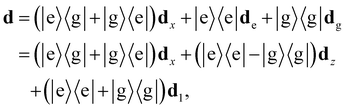
The full dipole operator for a single molecular emitter is given by
| |  | (1) |
where |e〉, |g〉 are the excited and ground state of the two-level electronic system,
dx is the transition dipole moment associated with the transition between ground and excited state of the dipole and
de(g) is the permanent dipole associated with the excited (ground) state of the dipole. The transition dipoles
dx may have a different orientation than the permanent dipoles associated with the vectors
. In
Fig. 1(d), we show a schematic of how such a chain may look.
We may then define the N-dipole chain single-excitation Hamiltonian as
| | | H = HS + Hopt + HI,opt + Hvib + HI,vib, | (2) |
where the system Hamiltonian describes the energies associated with just the dipoles, in units where
ħ = 1,
| |  | (3) |
where
σ(n)x = |0〉〈
n| + h.c and
σ(n)z = 2|
n〉〈
n| −
1, with

. We have also defined the transition energy of the
Nth site to be
ω0 and introduced a site-to-site detuning of
Δ, such that an energy gradient can be generated along the chain, with the highest energy at site 1. Here the mixed dipole coupling matrix
κijα,β is defined by
| | 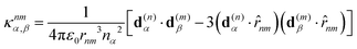 | (4) |
and is generated by the direct Coulombic dipole–dipole coupling with
![[r with combining circumflex]](https://www.rsc.org/images/entities/i_char_0072_0302.gif) nm
nm and
rnm being the unit direction vector and the magnitude of the distance between dipoles
n and
m, respectively. Further,
nz,
nx are the static and optical refractive index of the medium the dipoles are embedded respectively, screening the fields of each dipole.
86 Finally, |
n〉 is the state with the
nth dipole excited and |0〉 is the ground state of the
N dipole system.
The optical Hamiltonian term is of the form
| | 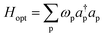 | (5) |
with
ωp representing the energy associated with the p-mode of the electromagnetic field and
a(†)p the p-modes annihilation (creation) operator. The optical bath couples to the dipoles through the interaction Hamiltonian
| | 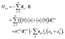 | (6) |
where
fp determines the strength with which the p-photon mode couples to the dipoles with vector dipole
dn with polarisation vector
ep. For convenience of analysis, we have chosen to neglect the identity dipole term
d1, as has been done in.
87,88 The remaining permanent dipole
d(n)z, the so-called difference dipole – as it captures the difference in the permanent dipoles from the excited and ground state of the molecule – will be from this point on what we refer to when discussing the permanent dipoles of these systems. Neglecting
d1 can be justified by noting that
d1–
d1 terms contribute an identity term to the Hamiltonian and can be immediately discounted.
d1–
dz terms introduce a small shift of energy levels, which could be absorbed into the uncoupled Hamiltonian. Finally, the
d1–
dx terms effectively introduce weak site-level driving. However, compared to the energetic splitting between the ground and excited states of the individual dipole systems, these terms will have a very limited impact on the eigenstructure. Furthermore, it has been shown that
d1 decouples from the
E-field for a single dipole,
69 a similar unitary transformation could be done for all the dipoles here to remove the
d1 term from the interaction Hamiltonian. For these reasons and narrative simplicity, we neglect
d1 from our analysis.
We constrain the dipoles such that they maintain a nearest neighbour interaction of 30 meV for H-aggregate configurations, appropriate for around 2 nm separations of dipoles with radiative lifetimes of nanoseconds. In this case, they can be considered to be spatially indistinguishable by the local electromagnetic field for relevant optical frequencies (≈700 nm ≫ 2 nm). A discussion detailing the derivation of this Hamiltonian is given in the SI. Finally, each dipole couples to its own vibrational environment, with the corresponding Hamiltonian
| |  | (7) |
and
| | 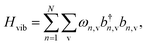 | (8) |
where
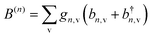
is the phonon displacement operator for the
nth dipole,
ωn,v,
gn,v and
b(†)n,v respectively represent the energy, the coupling strength, and the annihilation (creation) operator of the v-mode of the
nth dipole's vibrational bath.
By accounting for the permanent dipoles in these molecular systems, we have acquired multiple additional terms in our Hamiltonian. First, in the system Hamiltonian, we have new permanent-dipole permanent-dipole interactions, as well as permanent dipole-transition dipole interactions. The operator form of these interactions are σ(n)zσ(m)z and σ(n)xσ(m)z, respectively. The former term has the property of constituting a level shifting of the site energies of the molecular dipoles through a quasi-magnetic interaction. Depending on the sign of the interaction, the gaps between excitation manifolds can be modulated. Modulating the level splitting will affect the transitions between manifolds as given by Fermi's golden rule. Furthermore, the finite length of the chain entails that we will be able to induce asymmetric site-energy modulations along the chain. This can have a profound effect on the resonant conditions required for energy transport. This idea is laid out in Fig. 1(e). The second new term arising from permanent dipole-transition dipole interactions effectively induces driving of nearby dipoles based on the state of the dipole. However, by invoking a rotating wave approximation, these terms shall be neglected and their investigation left for future work. Furthermore, we have new interaction Hamiltonian terms arising from the interaction of the permanent dipoles with the electromagnetic field. The coupling to the electromagnetic field is through the σ(n)z operators, leading to qualitatively similar effects to vibrational dephasing. However, there are two pertinent differences between the two interactions. First, such ‘optical’ dephasing occurs through a shared environment between the molecular dipoles, and second, this interaction is with the same field as the transition dipoles, leading to additional decay channels for the system through non-additive effects. We explore these points in greater detail in the SI. There, we find that the addition of permanent dipoles allows for the accessibility of dark states through purely electromagnetic interactions, as well as modulations of the relevant decay rates strongly determined by the orientation of the constituent dipoles and rates that scale extensively compared to vibrational rates. However, due to weak coupling to the optical field, we anticipate that these effects will become more relevant for very large systems where the number of dipoles approaches the ratio of the vibrational and optical coupling strengths. We introduce notation for the various dipole configurations we consider throughout the rest of the text, this is depicted in Table 1. The notation is such that for a dipole configuration, e.g. ↑↑, the left arrow depicts the configuration of the transition dipole and the right arrow the permanent dipole; in the example given, these dipoles point in the same direction, orthogonal to the chain. In the following sections, we will restrict ourselves to the single excitation and ground state manifolds—though not necessary—this is sufficient for the weak injection regimes we study in the following. This amounts to replacing the full space system creation and annihilation operators by σ(n)+ → |n〉〈0| and σ(n)− → |0〉〈n|, where |0〉 is the zero excitation state and |n〉 is the state with the nth dipole excited.
Table 1 A graphical depiction (left columns) of the dipole configurations considered throughout this article and their corresponding text-based keys (right columns). For the rendered schematic, transition dipoles are depicted in blue and permanent dipoles in green. The first (left) character of the keys corresponds to transition dipole direction and the second (right) character denotes the permanent dipole configuration
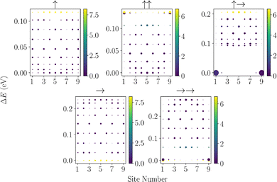
3 Eigenstructure
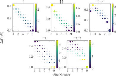
Having defined the many-body dipole Hamiltonian, it is informative to consider the eigenspectrum associated with the free Hamiltonian due to the permanent dipoles reorganising the bare energy levels. In Fig. 2, we depict a collection of such spectra for an emblematic set of dipole configurations in chains with 15 dipoles, where we have numerically diagonalised the system Hamiltonian. We have omitted the →↑ configuration due to similarities to the ↑↑ case, and not portraying additional interesting physics.
 |
| | Fig. 2 Plots of the eigenspectrum spreading across sites of a molecular chain, given different configurations of the permanent and transition dipoles. ΔE denotes the energy splitting from the lowest energy state in the single-excitation manifold. The optical brightness of each state is also depicted in the relative brightness of each state. | |
Another important factor for the efficiency of energy transport is the strength of the coupling between eigenstates with respect to the optical environment. Excitations in the chain can be lost due to spontaneous emission of photons, and the rate at which this occurs is determined by the brightness.29,77 For any particular eigenstate ψn within the single excitation manifold of the chain Hilbert space, we can determine its brightness by considering how the dipole-electromagnetic field interaction maps that state to the ground state and can be defined as
This is used to calculate the eigenstates' brightness, also shown in
Fig. 2. We can see that the vast majority of the eigenstates are suppressed optically due to destructive interference between transition dipoles, and a single bright state exists, which accumulates the transition strength from these dark states.
When examining the dipole–dipole chain eigenspectrum, it is useful to separate the roles of the permanent and transition dipoles. Neglecting mixed transition–permanent dipole terms, the permanent dipole–permanent dipole interaction does not couple different site-basis states; instead, it simply shifts their energies, as seen from
| | 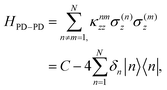 | (10) |
where

is the effective energy shift of the
nth site due to all the other sites permanent dipoles and

is a constant offset. A simple topological feature emerges: if the permanent-dipole couplings are dominated by nearest-neighbor terms and the dipoles are symmetric, then
δn =
δn+1 for all non-end sites. Only the first and last sites differ, as they each have a single neighbor, breaking the degeneracy at the chain boundaries by an amount proportional to the permanent dipole strength. We will see below how this boundary effect influences energy transport. The transition dipole–dipole interaction, by contrast, mixes the site basis and enables delocalization, an essential ingredient for transport in the Bloch–Redfield model discussed in the following section.
Using standard perturbation theory, the first-order correction to the eigenstates is
| | 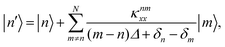 | (11) |
and the corresponding second-order energy correction is
| | 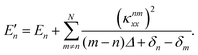 | (12) |
For small explicit detuning
Δ ≈ 0 the degree of end-site delocalization is therefore controlled by the ratio
κnmxx/
κnmzz. Moreover, the transition dipole-induced energy shifts inherit the same boundary-sensitive structure as the permanent dipole shifts, further enhancing this effect.
Returning to the numerically calculated eigenstates in Fig. 2. Consider the eigenstate's delocalisation for a H-aggregate configuration (↑). In the presence of no permanent dipoles and detuning in the system, all the eigenstates are delocalised across the chain, and we see that the optically brightest state lies at the highest energy in the single excitation manifold.82,89 Conversely, if we consider the configuration →→, we see that structure emerges from the spreading of eigenstates and the first and last sites are energetically the lowest in the manifold, with a large splitting between the rest of the central states within the manifold. This splitting is on the order of 10 s of meV. Such an eigenstructure may prove beneficial for transport as the relaxation processes associated with phonons, as well as permanent dipole-photon interactions, will guide the excitations towards these end nodes if an excitation makes it to the central manifold. Further to this, we can see that the specific transition dipole configuration positions the optically bright state in the central manifold, either positioning it at the bottom of the central manifold (as in configuration →→) or at the top (as in configuration ↑→). The positioning of this bright state is relevant for increasing chain sizes; its optical coupling strength is enhanced due to superradiance. As such, we would wish to position it at the top of the manifold, making it less accessible by absorption of phonons and thus introducing fewer optical losses. The other extreme is also achieved in the configuration ↑↑, wherein the end sites are at the top of the manifold, and we anticipate that such a configuration will have prohibitive transport as excitations are trapped along the chain within the central manifold.
Beyond simply guiding excitations to the end sites via relaxation processes, due to the splitting in the manifold being on the order of 10–100 meV we also anticipate that this structuring will make these permanent dipole chains more robust to static disorder of the site energies, as a large fluctuation would be required to significantly reorganise the energy levels. Similarly, small fluctuations in the local geometry of the dipoles do not greatly modify the eigenenergy structure. This is due to its origin from the asymmetry of the end dipoles coupling to fewer dipoles than dipoles towards the centre of the chain. Conversely, too large a separation between the end sites and the central manifold could be prohibitive for thermal fluctuations to promote excitations onto the central manifold. This will be explored further in Section 5. Alternatively, if one were in such a system where extraction was taken from within the central manifold and not from the end site, we would expect that the regimes with the lower central manifold would perform significantly better.
4 Open quantum systems modelling
In order to compare different dipole chain configurations we model the open quantum dynamics of these by utilising a weak-coupling Born–Markov approximation leading to the Bloch–Redfield equations.29 Such a master equation generates non-unitary dynamics for the reduced density matrix of the quantum dipoles due to decoherence and relaxation into the vibrational and photon baths. The Bloch-Redfield equation takes the form| | 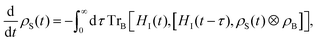 | (13) |
where HI(t) = HI,opt(t) + HI,vib(t), and using that S(t) denotes an operator S in the interaction picture. Noting that we can decompose our interaction Hamiltonian 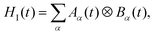 where operators Aα and Bα act on the chain system and baths, respectively, we can rewrite the second term on the right-hand side of the Bloch–Redfield master equation as
| | 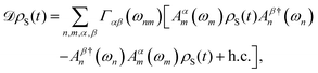 | (14) |
where Aαn are projections of Aα onto the nth eigenstate of the system Hamiltonian HS and Γαβ are the rates associated with the transition between eigenstates with energy ωn and ωm due to the interactions Bα and Bβ, and it is sampled at ωmn = ωm – ωn and h.c. is the Hermitian conjugate. These rate functions are related to the bath operators by Fourier transforms of the two-time correlations| | 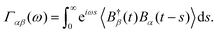 | (15) |
Under the assumption of thermalised environments, these correlation functions decompose into linear combinations of rates for both the optical and vibrational baths and are of the form| | 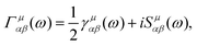 | (16) |
where μ ∈ {v, o}. The real-valued component γμnm is associated with the rate of the transition and the imaginary component Sμnm is associated with a Lamb shift which we neglect due to the inclusion of dipole–dipole couplings90 and the symmetric vibrational environments.91 The remaining rate contribution then takes the formwhere Jμ(ω) is the spectral density associated with the bath and N(ω) is related to the Bose–Einstein distribution n(ω) = 1/(exp![[thin space (1/6-em)]](https://www.rsc.org/images/entities/char_2009.gif) βω − 1) for the bosonic vibrational and optical bath modes, as
βω − 1) for the bosonic vibrational and optical bath modes, as| | 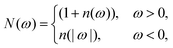 | (18) |
where β = 1/kBT is the inverse temperature. These relations ensure detailed balance for our transitions. To remove effects associated with specific structures in the environment leading to enhancements, we choose flat spectral densities for both the phonon and optical environments such thatwhere we have taken γo = 1 µeV and γv = 1 meV, which are typical for biomolecular systems with nanosecond lifetimes. For specific condensed phase molecular systems, these values may be modulated47 due to polarisation of the material environment. For a general linear dielectric environment γo → nrγo, where nr is the refractive index of the dielectric medium, a common approach for modelling protein environments86 and solid-state systems. In realistic condensed-phase systems, the degree of delocalization depends on system-specific factors such as dipole strengths, molecular geometry, solvent environment, and the magnitudes of static and dynamic disorder; sufficiently strong disorder may drive localization and lead to hopping-dominated transport. The key competition is between the transition–dipole couplings and the disorder fluctuations, with the former being enhanced by reduced subunit spacing. Our framework captures the resulting interplay between permanent and transition dipoles within plausible molecular arrangements. As we explore below, the qualitative effects we identify persist even in regimes where static disorder exceeds the dipole couplings. Due to the decomposition of the correlations into optical and vibrational contributions, we too can decompose the Redfield dissipator into a linear combination of optical and vibrational dissipators as
We employ a model for extracting excitons from the chain system for conversion to useful energy. This is achieved by adding a Lindblad dissipator to the end site of the chain
| | 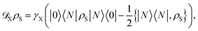 | (21) |
where
γX is the rate of extraction from the end site. Such a transport process can be considered as excitations reaching a reaction site and then being utilised for chemical processes relevant to light-harvesting systems or conversion into an electrical current in photovoltaic systems.
Similarly, we introduce an excitation injection process via another Lindblad operator, causing incoherent excitations to enter the first site of the chain. This takes the form
| | 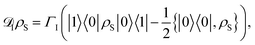 | (22) |
where
ΓI is the rate of injection. This models the input of excitations into the network.
In many realistic physical systems, non-radiative decay processes will lead to a loss of excitations as they are transported along the chain, which can be caused by the emission of many phonons through heat.28 In this model, we incorporate non-radiative decay by adding a Lindblad decay process at each site in the system
| |  | (23) |
with
ΓNR the rate of non-radiative decay.
We can then construct the total master equation for the reduced density matrix of the dipole ring by summation of these dissipators
| | 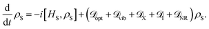 | (24) |
The injection and extraction processes generate an effective quantum (flow) heat engine that enables the study of relevant functional properties of these transport networks.
74 We use as a figure of merit the induced steady state current through the end of the chain, which is given by ref.
34,
36,
74,
91 and
92where 〈|
N〉〈
N|〉 is the expectation value of the steady state population for the excited state of the final site in the chain. The steady state is calculated by finding the nullspace of the Liouvillian operator
![[scr D, script letter D]](https://www.rsc.org/images/entities/char_e523.gif)
defined by

. This steady-state current quantifies the number of excitons extracted per unit time when the system is in equilibrium. Whilst the Bloch-Redfield formalism developed here is necessarily a weak-coupling master equation, it can offer powerful explanatory power for qualitatively understanding the dynamics of a large range of systems relevant to energy transport systems.
93–95
5 Energy transport
We now utilise the open quantum systems model outlined above to compare different setups for the relative orientations between the permanent dipoles and the transition dipoles within the chain. In the following, we focus on studying some of the most obvious and generic features of the model that can deleteriously impact the transport in these systems.
For all the results in this section, unless specified, we have utilised the parameters laid out in Table 2, with a default of equal relative magnitude of permanent dipoles to the transition dipoles as indicated by the value dSCz = 1. The inclusion of a finite level of non-radiative decay is useful as it allows for the neglecting of explicit discussions about the speed at which energy transport occurs. This is because, in those systems in which transport is slow (compared to the non-radiative decay rates), the steady-state current will be suppressed.
Table 2 Table of the parameters used in the simulations, unless specified otherwise
| Parameter |
Value |
|
The nearest neighbour coupling in an H-aggregate (↑) setting an effective distance scale.
|
|
ε
|
1.8 eV |
|
T
o
|
300 K |
|
T
v
|
300 K |
|
Γ
I
|
10−6 meV |
|
γ
X
|
0.002 meV |
|
N
|
9 |
|
Γ
NR
|
0.001 meV |
|
Δ
|
0 |
|
κ
ii+1
x,xa |
30 meV |
|
d
SC
z
|
1 |
5.1 Length of molecular chain
We start by considering molecular chains of varying length made up of N molecular dipole elements. In Fig. 3, we show how the transport is modulated for various configurations of the permanent and transition dipoles by calculating the steady-state current due to extraction at the final site in the chain. We can readily see that across the range of chain lengths N, the J-aggregate transition dipole and permanent dipole system (→→) greatly outperforms the J-aggregate transition dipole configuration without permanent dipoles (→), exhibiting an order of magnitude greater exciton transport. Showing that permanent dipoles can introduce new energetic pathways for excitations to transfer through the network. Further across a collection of chain lengths, the J–J aggregate system yields the highest degree of transport. The discrepancy between different dipole configurations can be understood by the relative splitting between the central and end-state energies, too large a splitting makes transport prohibitive. Conversely, we can see that the dipole configuration ↑↑ performs poorly which has its central manifold lower in energy compared with the edge sites, leading to the trapping of excitations. Furthermore, we can see that the drop-off in the current across the chain is also greatly modulated with chain length, for some optimal configurations we see very little decay in this steady-state current. We see fluctuations for the ↑→ configuration for small chain lengths due to the spacing between the central manifold and the end sites fluctuating for short chains, this effect smoothens out for larger chains due to the 1/r3 dipole–dipole coupling reducing the impact of additional dipoles in the chain to any particular chains energy splitting, furthermore, the splitting it induces is large compared to thermal fluctuations and thus can be prohibitive to exciton transport, causing it to fall off quickly.
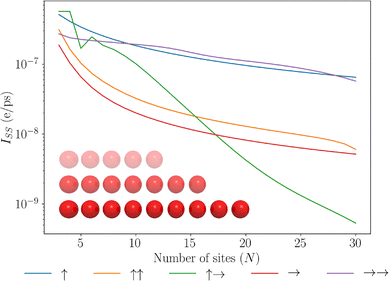 |
| | Fig. 3 A plot of the steady state current against different lengths of molecular dipole chains. Different configurations of transition (left) and permanent (right) dipoles are considered. See Table 1, for details of the legend. The inset depicts a collection of dipole chains of different lengths and equal dipole energies. | |
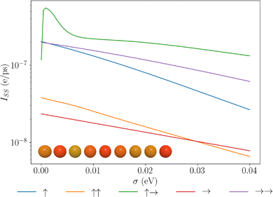
5.2 Static noise
In most physical systems relevant to condensed matter physics, solid-state and biological settings, we anticipate that there will be some degree of static disorder in the site energies across the chain, due to local fluctuations of structure and orientation about the positions of the dipoles.96,97 To understand the implications of this static disorder, we now consider the effects of static disorder and how permanent dipoles play an important role in mitigating these effects. In Fig. 4, we see that the dipole chains are relatively robust against moderate static noise in the system. This can be understood from the eigenspectrum, seen from Fig. 2, that due to strong dipole–dipole couplings, structure appears in these systems with separations between eigenstates on the order of 10 s of meV, where a large energy gap must be overcome to modulate the overall structure in the eigenspectrum greatly. The most intriguing feature is observed for the ↑→ configuration, wherein a small degree of static disorder conveys a large increase in the current. We can understand this by looking at the eigenspectra for such fluctuations. Fig. 5, shows the eigenspectrum localisation for a single instance of 0.1 meV fluctuations in the site basis. Almost all of the configurations exhibit no change at this level. However, the ↑→ configuration exhibits strong localisation of the end site eigenstates that were brought about due to a perfect zero detuning between these states and small but non-zero coupling. This localisation may seem detrimental to transport, but localising the two end sites allows for slight enhancements of the end sites' delocalisation between adjacent sites, enhancing their ability to enter the central manifold states. This is exemplified by considering the zero-temperature environment, such that no thermal fluctuations may occur. This is shown in the SI, wherein we see the opposite effect occurring for this configuration, small static noise greatly hinders transport as the excitations have no mechanism to enter the central manifold. This zero detuning long-ranged delocalised state is non-physical as a finite degree of static noise will always be present and as such this configuration proves unstable to this noise. Furthermore, after the initial jump, the energy transport is the most weakly suppressed by the static disorder over the regime studied here. We can also see that the →→ configurations outperform the no permanent dipole case across almost the entire range of static noise introduced, exhibiting slow decay with respect to the static disorder. These enhancements can be almost an order of magnitude greater than those in the transition dipole J-aggregate setup. Furthermore, we anticipate the same trends to be true for geometric disorder, due to the preservation of the eigenenergy structure under moderate geometric fluctuations as seen in the SI.
 |
| | Fig. 4 Plots of the steady state current due to extraction of the end site of a molecular dipole chain for different dipolar configurations. Varying the magnitude of static noise between site energies. Results are an average of 1000 different random iterations wherein all energy levels are shifted by a zero mean normally distributed value with standard deviation σ. The inset shows a dipole chain, with colours denoting the transition energies of the dipoles, the transition energies for a single sample are uniformly distributed as shown here. | |
 |
| | Fig. 5 Plots of the eigenstates localisation onto the site basis and the associated optical brightness of each state for different molecular dipole configurations. Results are for a single instantiation of static noise at a level of 0.1 meV. | |
5.3 Detuning
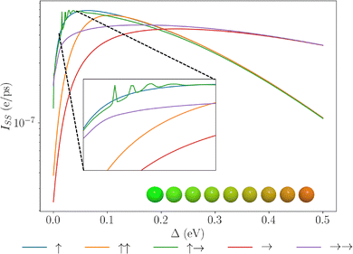
Similarly, it is natural to consider dipolar chains with explicit energy level biases such that phonon-relaxation processes can guide excitations along an energetic gradient.34,36 In Fig. 6, we show how different magnitudes of detuning from site to site impact the effectiveness of each of the dipole configurations.
 |
| | Fig. 6 Plots of the steady state current due to the extraction of the end site of a molecular dipole chain for different dipolar configurations. Varying the site-to-site detuning introduces an energetic gradient. The inset shows a dipole chain, with colours denoting the transition energies of the dipoles, going from green (high energy) to red (low energy). | |
Unsurprisingly, introducing a bias along the chain improves exciton transport, though this benefit is only up to a certain magnitude of detuning before eigenstate localisation overwhelms any possible transport between the eigenstates. For large detuning, the dominant effects are due to the transition dipole as evidenced by the saturation of the curves to the purely transition dipole ones. This is due to the detuning exceeding the permanent dipole energy reorganisation. Intriguingly, the ↑→ configuration exhibits sharp-peaked features. This can be understood by considering the eigenspectrum, of this state: as we increase the site-to-site detuning, due to the strong permanent-dipole–permanent-dipole couplings, we introduce energetic barriers in the spectrum wherein the dipole–dipole coupling is of a similar magnitude to the detuning. This is depicted in Fig. 7, where the ↑→ configuration, can induce a local energetic barrier into the chain due to strong dipole–dipole coupling. The other configurations do not have sufficient dipole–dipole coupling strengths to induce such structures and as such do not admit such barriers. The effect of site-level energy barriers has been previously explored in ref. 34 and has been shown to aid in reducing radiative decay through dark-state protection and thus enhancing energy transport. We see strong oscillations about these local maxima, and when the detuning overcomes the dipole–dipole coupling >70 meV, we note that these bumps can no longer exist in these systems. This unique effect emerging naturally within these systems is further evidence that permanent dipoles play an important effect in the nature of energy transport in dipolar chains.
 |
| | Fig. 7 Distribution of eigenstates of molecular dipole chains onto the local site basis for an optimum detuning of Δ = 48 meV as determined from Fig. 6. | |
5.4 Non-radiative decay
Many physical systems for which our model is relevant will suffer from additional non-radiative recombination processes during transport that are, in principle, avoidable but, in practice, often dominant over the (intrinsically unavoidable) radiative loss mechanism.98,99 Such mitigation strategies include the removal of impurities in fabricated solid-state systems, cooling the system to reduce stimulated phonon effects or in molecular systems utilising strong dipole couplings between sites to inhibit the formation of localised polarons.100 Since non-radiative leakage rates may span many orders of magnitude depending on the physical system in question, we consider a large scale of non-radiative decay rates. In Fig. 8, we investigate the effects of non-radiative decay along the chain with different rates. We can see that the J–J aggregate system experiences significantly lower losses due to the non-radiative rates. We can understand this by considering the time evolution of the population into the end site. In the SI, we show the time evolution for zero non-radiative decay rate, and we see that the J–J system reaches a high value for the end site population the fastest amongst the various configurations, which enables excitations to be extracted before excitons are lost due to radiative and non-radiative decay.
 |
| | Fig. 8 Plots of the steady state current due to extraction of the end site of a molecular dipole chain for different dipolar configurations. Varying the strength of non-radiative decay in the system. Inset depicts site local non-radiative decay across dipole chain. | |
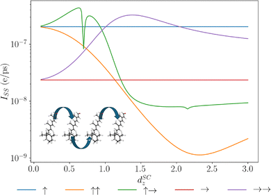
5.5 Permanent dipole strength
Another relevant degree of freedom within these permanent dipole chain systems is the magnitude of the permanent dipoles, and then how this impacts the transport efficiency. Different molecular systems that form the transport network will possess different permanent dipoles associated with the specific structure of their molecular orbitals. The magnitude of these permanent dipoles can vary starkly: e.g., retinal, a common chromophore, possesses permanent dipoles of 15.6 D101 whereas moiré excitons possess permanent dipoles up to 48 D.60 From the eigenstructures seen previously in Fig. 2, we noted that the permanent dipoles can arrange the energy eigenspectrum preferentially, by lowering states in the centre of the chain. However, if that splitting becomes too large, the thermal fluctuations required to promote states from the central manifold states to the end states may be suppressed. To understand the effects, we have plotted the results of simulations for chains with varying permanent dipole strength in Fig. 9. Here, we see a few interesting properties. First, we note a clear non-monotonic effect in the permanent dipole magnitude across the configurations. This can be understood by considering two competing effects. The permanent dipole-permanent dipole interactions single out the two end sites, and the magnitude of the permanent dipoles is directly proportional to the splitting. For small splitting between the central manifold and end sites, thermal fluctuations will act almost bi-directionally [as n(ω) ≫ 1], for the raised central manifold enhancing transport, and will quickly populate the central manifold for the lowered central manifold systems, trapping excitations and thus reducing transport. Growing spacing between the end sites and the central manifold leads to a breakdown of the bidirectional flow and a breaking of delocalisation of the end sites with central manifold states, inhibiting transport into the centre of the chain. This breakdown of delocalisation into the centre of the chain does, however, increase delocalisation directly between the two end sites as they become further separated from the other sites' energies.
 |
| | Fig. 9 Plots of the steady state current due to extraction of the end site of a molecular dipole chain for different dipolar configurations. Varying the relative strength of the permanent dipoles to the transition dipoles. Inset shows a chain of chromophore retinal, retinal has been shown to possess large permanent dipole moments in the excited state 15.6 D.101 | |
We also note the sharp feature for the ↑→ configuration for permanent dipole strength of ≈0.697 that of the transition dipole strength. This feature can be directly understood by determining the eigenspectrum for this configuration. At this value, we find that the bottom two states are delocalised dark and bright states between the end sites that become entirely degenerate and the phonon-assisted transport has no support at zero frequency under our choice of spectral density. This feature again exhibits the rich properties that permanent dipoles can have on energy transport.
We have refrained from taking the permanent dipole strengths arbitrarily large as this could break down the efficacy of the perturbative framework deployed in this work. Previous work has studied the effects of strong permanent dipole effects and has shown that these can lead to optical decay rate suppression.69
5.6 Phonon coupling strength
The strength of phonon interactions can vary greatly depending on the system considered, in solid-state systems, such as quantum dots, the reorganisation energy of the environment can be 10 s of µeV,102 conversely, for biological systems this can be as large as 100 s of meV.103 Therefore, we perform simulations across many orders of magnitude by scaling γv → αγv and varying α. To study the celebrated Environmental Noise-Assisted Quantum Transport (ENAQT) effect104–108 we fix the length of the chain to N = 7 as in ref. 109. The results of these simulations are shown in Fig. 10, and we see many intriguing features within these results. First, in Fig. 10(a) we show the current generated for the standard configuration with extraction taken from the end site. Here we note that there is a monotonic behaviour for most configurations except for the ↑→ configuration that exhibits a local maximum ENAQT peak. All configurations perform best at lower vibrational couplings. This can be understood by the delocalised states that form in the zero disorder systems meaning it is easier to extract directly from end sites. In Fig. 10(b), we consider extraction from the penultimate site in the chain as in ref. 109, as this breaks the inversion symmetry in the network. Here, we see that for the H-aggregate system without permanent dipoles and the double H-aggregate system, the ENAQT peaks appear to show an optimal regime for environmental noise. However, this is in no sense a general feature of these networks, with many showing monotonic losses due to vibrational coupling. Furthermore, we can see that the J-aggregate systems without permanent dipoles no longer exhibit an ENAQT peak due to the additional dissipation channels through radiative and non-radiative decay. In the SI, we explore the same scenario as in Fig. 10(b) without non-radiative decay, we see similar features to the case with non-radiative decay, though with some of the configurations exhibiting multiple peaks in the current akin to the effects seen in ref. 72. We also removed all exciton loss channels and we see the restoration of the ENAQT peak for the J-aggregate transition dipole system, but this feature is not present for systems with permanent dipoles. These results suggest that there is a very strong interplay between vibrational and radiative/non-radiative decay when considering optimal environmental noise conditions. We note that a full analysis of strong coupling to the bath would require a framework beyond the second-order perturbations developed here, and we anticipate suppression of transport at higher coupling strengths due to polaron formation.91 Such a framework could include numerically exact process tensor approaches,110–112 or variational master equation approaches.100
 |
| | Fig. 10 Plots of the steady state current due to extraction of the end site of a molecular dipole chain for different dipolar configurations. Varying the relative strength of the vibrational coupling to the dipoles. (a) With extraction from the end site (b) With extraction from the penultimate site. The inset depicts a dipole chain with independent vibrational effects at each site along the chain. | |
6 Conclusion
In this article, we have studied the effects of permanent dipoles in molecular systems on their ability to transport excitations along a wire. We have shown that permanent dipoles allow for the effective structuring of eigenenergies in the single excitation manifold, which are suitable for enabling the transport of excitations. This was then followed by a robust study of how various factors, that are detrimental to transport such as non-radiative decay, local static noise in energy levels, detunings and vibrational decay rates still allowed for molecular systems with permanent dipoles to outperform, in some cases, those without in their ability to admit excitation transport. This advantage was conveyed by the generation of a central manifold separated from the end sites where injection and extraction are performed. This separation of localised eigenstates onto the end sites has been shown to enhance energy transport by removing population nodes in the chain.109 Such an energy structure is preserved under moderate static noise in on-site energy splittings and makes permanent dipole configurations more robust to this noise compared to chains that only possess transition dipoles. For detuned chains, permanent dipoles can introduce local energetic barriers that enhance transport efficiency,34 manifesting in a multiply peaked current profile. For systems with a large degree of non-radiative decay, permanent dipoles enhance the speed of transport, overcoming the site-local losses, greatly increasing the steady-state current available. A natural question to ask is whether such dipole configurations occur in any molecular transport systems. In the case of pseudoisocyanin dyes, collective large permanent dipoles have been seen.83 This is a general feature of many dye and chromophore molecules, such as bacteriachlorophyll, which possesses permanent dipoles and has been found and measured at a relative angle to the transition dipole of around 11°, almost entirely parallel. As well as permanent dipole strengths on the same order of magnitude as the transition dipoles.113 Similar permanent dipoles are seen for the chromophore in phycobilisomes, suggesting that permanent dipoles may have a key role to play in energy transport. Here, we have studied highly symmetric configurations of dipole geometries. It is natural to expect that optimised configurations of permanent dipoles and transition dipoles could have greatly enhanced transport capabilities and that nature may exploit such configurations. Furthermore, for the more complex configurations, techniques of dipole–dipole interaction engineering could be deployed to induce the desired eigenstructure.114,115 Another outlook for this work would be to consider the many-exciton currents wherein new features such as exciton–exciton annihilation are expected to play an important role.99 Finally, by leveraging mature molecular dynamics simulations, one could directly compute the relevant dipole Hamiltonians needed to study specific molecular systems and directly validate the mechanisms discussed here. The effects of permanent dipoles are often neglected in quantum optics studies, and here we have shown that they can play an important role in charge transport, thus warranting their further study.
Conflicts of interest
There are no conflicts to declare.
Data availability
The data supporting this article has been generated using the open source package QuTiP116 and all parameters used have been included within Table 2.
The data supporting this article have been included as part of the supplementary information (SI). Supplementary information is available. These include a derivation of the Hamiltonian used, additional rate calculations, effects of detuning at zero temperature, the dynamics of excitons with non-radiative decay and further ENAQT studies. See DOI: https://doi.org/10.1039/d5cp04076k.
Acknowledgements
A. Burgess and E. M. Gauger thank the Leverhulme Trust for support through grant number RPG-2022-335.
Notes and references
- D. Balzer and I. Kassal, Chem. Sci., 2024, 15, 4779–4789 RSC.
- G. D. Scholes, Annu. Rev. Phys. Chem., 2003, 54, 57–87 CrossRef CAS.
- W. P. Bricker, J. L. Banal, M. B. Stone and M. Bathe, J. Chem. Phys., 2018, 149, 024905 CrossRef PubMed.
-
T. L. Andrew and T. M. Swager, Structure Property Relationships for Exciton Transfer in Conjugated Polymers, John Wiley & Sons, Ltd, 2011, ch. 10, pp. 271–310 Search PubMed.
- F. C. Spano and C. Silva, Annu. Rev. Phys. Chem., 2014, 65, 477–500 CrossRef CAS PubMed.
-
H. van Amerongen, R. van Grondelle and L. Valkunas, Photosynthetic Excitons, World Scientific, 2000 Search PubMed.
-
R. Blankenship, Molecular Mechanisms of Photosynthesis, Wiley, 2021 Search PubMed.
-
J. Nelson, The Physics Of Solar Cells, World Scientific Publishing Company, 2003 Search PubMed.
- H.-G. Duan, V. I. Prokhorenko, R. J. Cogdell, K. Ashraf, A. L. Stevens, M. Thorwart and R. J. D. Miller, Proc. Natl. Acad. Sci. U. S. A., 2017, 114, 8493–8498 CrossRef CAS.
- A. Halpin, P. J. M. Johnson, R. Tempelaar, R. S. Murphy, J. Knoester, T. L. C. Jansen and R. J. D. Miller, Nat. Chem., 2014, 6, 196–201 CrossRef CAS PubMed.
- P. Nalbach, D. Braun and M. Thorwart, Phys. Rev. E: Stat., Nonlinear, Soft Matter Phys., 2011, 84, 041926 CrossRef CAS PubMed.
- S. Tomasi and I. Kassal, J. Phys. Chem. Lett., 2020, 11, 2348–2355 CrossRef CAS PubMed.
- J. Strümpfer, M. Åžener and K. Schulten, J. Phys. Chem. Lett., 2012, 3, 536–542 CrossRef PubMed.
- M. O. Scully, Phys. Rev. Lett., 2010, 104, 207701 CrossRef PubMed.
- J. Schachenmayer, C. Genes, E. Tignone and G. Pupillo, Phys. Rev. Lett., 2015, 114, 196403 CrossRef.
- G. D. Scholes, G. R. Fleming, L. X. Chen, A. Aspuru-Guzik, A. Buchleitner, D. F. Coker, G. S. Engel, R. van Grondelle, A. Ishizaki, D. M. Jonas, J. S. Lundeen, J. K. McCusker, S. Mukamel, J. P. Ogilvie, A. Olaya-Castro, M. A. Ratner, F. C. Spano, K. B. Whaley and X. Zhu, Nature, 2017, 543, 647–656 CrossRef CAS PubMed.
- K. E. Dorfman, D. V. Voronine, S. Mukamel and M. O. Scully, Proc. Natl. Acad. Sci. U. S. A., 2013, 110, 2746–2751 CrossRef CAS.
- W. M. Brown and E. M. Gauger, J. Phys. Chem. Lett., 2019, 10, 4323–4329 CrossRef CAS PubMed.
- N. Werren, W. Brown and E. M. Gauger, PRX Energy, 2023, 2, 013002 CrossRef.
- J. Q. Quach, K. E. McGhee, L. Ganzer, D. M. Rouse, B. W. Lovett, E. M. Gauger, J. Keeling, G. Cerullo, D. G. Lidzey and T. Virgili, Sci. Adv., 2022, 8, eabk3160 CrossRef CAS.
- K. D. B. Higgins, S. C. Benjamin, T. M. Stace, G. J. Milburn, B. W. Lovett and E. M. Gauger, Nat. Commun., 2014, 5, 4705 CrossRef CAS PubMed.
- K. D. B. Higgins, B. W. Lovett and E. M. Gauger, J. Phys. Chem. C, 2017, 121, 20714–20719 Search PubMed.
- Y. Zhang, S. Oh, F. H. Alharbi, G. S. Engel and S. Kais, Phys. Chem. Chem. Phys., 2015, 17, 5743–5750 RSC.
- G. D. Scholes, Proc. R. Soc. A, 2020, 476, 20200278 CrossRef PubMed.
- N. C. Chávez, F. Mattiotti, J. A. Méndez-Bermúdez, F. Borgonovi and G. L. Celardo, Phys. Rev. Lett., 2021, 126, 153201 CrossRef PubMed.
- O. V. Mikhnenko, P. W. M. Blom and T.-Q. Nguyen, Energy Environ. Sci., 2015, 8, 1867–1888 RSC.
- D. Balzer and I. Kassal, J. Phys. Chem. Lett., 2023, 14, 2155–2162 CrossRef CAS.
- V. Perebeinos and P. Avouris, Phys. Rev. Lett., 2008, 101, 057401 CrossRef.
-
H.-P. Breuer and F. Petruccione, et al., The Theory of Open Quantum Systems, Oxford University Press on Demand, 2002 Search PubMed.
- P. Kirton, M. M. Roses, J. Keeling and E. G. Dalla Torre, Adv. Quantum Technol., 2019, 2, 1800043 CrossRef.
- S. Baghbanzadeh and I. Kassal, J. Phys. Chem. Lett., 2016, 7, 3804–3811 CrossRef CAS PubMed.
- R. H. Dicke, Phys. Rev., 1954, 93, 99–110 CrossRef CAS.
- A. Fruchtman, R. Gómez-Bombarelli, B. W. Lovett and E. M. Gauger, Phys. Rev. Lett., 2016, 117, 203603 CrossRef.
- S. Davidson, A. Fruchtman, F. A. Pollock and E. M. Gauger, J. Chem. Phys., 2020, 153, 134701 CrossRef PubMed.
- A. Mattioni, F. Caycedo-Soler, S. F. Huelga and M. B. Plenio, Phys. Rev. X, 2021, 11, 041003 Search PubMed.
- S. Davidson, F. A. Pollock and E. Gauger, PRX Quantum, 2022, 3, 020354 CrossRef.
-
Z. Ficek and S. Swain, Quantum Interference and Coherence: Theory and Experiments, Springer Science & Business Media, 2005, vol. 100 Search PubMed.
- A. J. Leggett, S. Chakravarty, A. T. Dorsey, M. P. Fisher, A. Garg and W. Zwerger, Rev. Mod. Phys., 1987, 59, 1 CrossRef.
- G. S. Agarwal, Quantum Opt., 1974, 1–128 Search PubMed.
- P.-H. Chung, C. Tregidgo and K. Suhling, Methods Appl. Fluoresc., 2016, 4, 045001 CrossRef PubMed.
- C. Filippi, F. Buda, L. Guidoni and A. Sinicropi, J. Chem. Theory Comput., 2012, 8, 112–124 CrossRef PubMed.
- V. Kovarski and O. Prepelitsa, Opt. Spectrosc., 2001, 90, 351–355 CrossRef.
- J. Deiglmayr, A. Grochola, M. Repp, O. Dulieu, R. Wester and M. Weidemüller, Phys. Rev. A: At., Mol., Opt. Phys., 2010, 82, 032503 CrossRef.
- R. Guérout, M. Aymar and O. Dulieu, Phys. Rev. A: At., Mol., Opt. Phys., 2010, 82, 042508 CrossRef.
- C.-Y. Lin and S. G. Boxer, J. Am. Chem. Soc., 2020, 142, 11032–11041 Search PubMed.
- B. Jagatap and W. J. Meath, J. Opt. Soc. Am. B, 2002, 19, 2673–2681 CrossRef.
- J. Gilmore and R. H. McKenzie, J. Phys.: Condens. Matter, 2005, 17, 1735 CrossRef.
- L. Garziano, V. Macr, R. Stassi, O. Di Stefano, F. Nori and S. Savasta, Phys. Rev. Lett., 2016, 117, 043601 CrossRef PubMed.
- I. Y. Chestnov, V. Shakhnazaryan, I. A. Shelykh and A. P. Alodjants, JETP Lett., 2016, 104, 169–174 CrossRef.
- M. Shim and P. Guyot-Sionnest, J. Chem. Phys., 1999, 111, 6955–6964 CrossRef.
- M. Antón, F. Carreño, O. Calderón, S. Melle and E. Cabrera, J. Opt., 2016, 18, 025001 Search PubMed.
- P. Fry, I. Itskevich, D. Mowbray, M. Skolnick, J. Barker, E. O'Reilly, L. Wilson, P. Maksym, M. Hopkinson and M. Al-Khafaji,
et al.
, Phys. E, 2000, 7, 408–412 Search PubMed.
- I. Y. Chestnov, V. A. Shahnazaryan, A. P. Alodjants and I. A. Shelykh, ACS Photonics, 2017, 4, 2726–2737 CrossRef.
- P. W. Fry, I. E. Itskevich, D. J. Mowbray, M. S. Skolnick, J. J. Finley, J. A. Barker, E. P. O'Reilly, L. R. Wilson, I. A. Larkin, P. A. Maksym, M. Hopkinson, M. Al-Khafaji, J. P. R. David, A. G. Cullis, G. Hill and J. C. Clark, Phys. Rev. Lett., 2000, 84, 733 CrossRef PubMed.
- M. A. Antón, S. Maede-Razavi, F. Carreño, I. Thanopulos and E. Paspalakis, Phys. Rev. A, 2017, 96, 063812 CrossRef.
- A. Patane, A. Levin, A. Polimeni, F. Schindler, P. Main, L. Eaves and M. Henini, Appl. Phys. Lett., 2000, 77, 2979–2981 CrossRef CAS.
- R. J. Warburton, C. Schulhauser, D. Haft, C. Schäflein, K. Karrai, J. M. Garcia, W. Schoenfeld and P. M. Petroff, Phys. Rev. B: Condens. Matter Mater. Phys., 2002, 65, 113303 CrossRef.
- I. A. Ostapenko, G. Hönig, C. Kindel, S. Rodt, A. Strittmatter, A. Hoffmann and D. Bimberg, Appl. Phys. Lett., 2010, 97, 063103 CrossRef.
- L. A. Jauregui, A. Y. Joe, K. Pistunova, D. S. Wild, A. A. High, Y. Zhou, G. Scuri, K. D. Greve, A. Sushko, C.-H. Yu, T. Taniguchi, K. Watanabe, D. J. Needleman, M. D. Lukin, H. Park and P. Kim, Science, 2019, 366, 870–875 CrossRef CAS PubMed.
- S. Feng, A. J. Campbell, M. Brotons-Gisbert, D. Andres-Penares, H. Baek, T. Taniguchi, K. Watanabe, B. Urbaszek, I. C. Gerber and B. D. Gerardot, Nat. Commun., 2024, 15, 4377 CrossRef CAS PubMed.
- G. Guarnieri, M. Kolár and R. Filip, Phys. Rev. Lett., 2018, 121, 070401 CrossRef CAS.
- Y. S. Greenberg, Phys. Rev. B: Condens. Matter Mater. Phys., 2007, 76, 104520 CrossRef.
- J. B. Gilmore and R. H. McKenzie, Chem. Phys. Lett., 2006, 421, 266–271 CrossRef CAS.
- M. Schut, H. Bosma, M. Wu, M. Toroš, S. Bose and A. Mazumdar, Phys. Rev. A, 2024, 110, 022412 CrossRef CAS.
- M. Freed, D. M. Rouse, A. Rocco, J. S. Al-Khalili, M. Florescu and A. Burgess, New J. Phys., 2025 DOI:10.1088/1367-2630/ae2a61.
- R. Román-Ancheyta, M. Kolár, G. Guarnieri and R. Filip, Phys. Rev. A, 2021, 104, 062209 CrossRef.
- A. Purkayastha, G. Guarnieri, M. T. Mitchison, R. Filip and J. Goold, npj Quantum Inf., 2020, 6, 1–7 CrossRef.
- A. Mandal, S. Montillo Vega and P. Huo, J. Phys. Chem. Lett., 2020, 11, 9215–9223 CrossRef CAS.
- A. Burgess, M. Florescu and D. M. Rouse, AVS Quantum Sci., 2023, 5, 031402 CrossRef.
- R. Car and M. Parrinello, Phys. Rev. Lett., 1985, 55, 2471–2474 CrossRef CAS PubMed.
- Y. Zhang, A. Wirthwein, F. H. Alharbi, G. S. Engel and S. Kais, Phys. Chem. Chem. Phys., 2016, 18, 31845–31849 RSC.
- A. R. Coates, B. W. Lovett and E. M. Gauger, Phys. Chem. Chem. Phys., 2023, 25, 10103–10112 RSC.
- A. Kolli, A. Nazir and A. Olaya-Castro, J. Chem. Phys., 2011, 135, 154112 CrossRef.
- N. Killoran, S. F. Huelga and M. B. Plenio, J. Chem. Phys., 2015, 143, 155102 CrossRef CAS.
- S.-J. Yang, D. J. Wales, E. J. Woods and G. R. Fleming, Nat. Commun., 2024, 15, 8763 CrossRef CAS.
- C. Leonardo, S.-J. Yang, K. Orcutt, M. Iwai, E. A. Arsenault and G. R. Fleming, J. Phys. Chem. B, 2024, 128, 7941–7953 CrossRef CAS.
- E. J. Dodson, N. Werren, Y. Paltiel, E. M. Gauger and N. Keren, J. R. Soc., Interface, 2022, 19, 20220580 CrossRef CAS PubMed.
- A. Ishizaki and G. R. Fleming, J. Chem. Phys., 2009, 130, 234111 CrossRef PubMed.
- M. R. Bryce, J. Mater. Chem. C, 2021, 9, 10524–10546 RSC.
-
D. Kim, Multiporphyrin arrays: Fundamentals and applications, Pan Stanford Publishing PTE. Ltd., 2011 Search PubMed.
- E. A. Weiss, M. J. Ahrens, L. E. Sinks, A. V. Gusev, M. A. Ratner and M. R. Wasielewski, J. Am. Chem. Soc., 2004, 126, 5577–5584 CrossRef CAS PubMed.
- N. J. Hestand and F. C. Spano, Chem. Rev., 2018, 118, 7069–7163 CrossRef CAS.
- T. Kobayashi, Mol. Cryst. Liq. Cryst. Sci. Technol., Sect. A, 1998, 314, 1–11 CrossRef CAS.
- S. M. Hart, W. J. Chen, J. L. Banal, W. P. Bricker, A. Dodin, L. Markova, Y. Vyborna, A. P. Willard, R. Haner, M. Bathe and G. S. Schlau-Cohen, Chem, 2021, 7, 752–773 CAS.
- S. Mandal, X. Zhou, S. Lin, H. Yan and N. Woodbury, Bioconjugate Chem., 2019, 30, 1870–1879 CrossRef CAS PubMed.
- L. Li, C. Li, Z. Zhang and E. Alexov, J. Chem. Theory Comput., 2013, 9, 2126–2136 CrossRef CAS PubMed.
- T. Hattori and T. Kobayashi, Phys. Rev. A: At., Mol., Opt. Phys., 1987, 35, 2733–2736 CrossRef CAS.
- J.-Y. Zhao, L.-G. Qin, X.-M. Cai, Q. Lin and Z.-Y. Wang, Chin. Phys. B, 2016, 25, 044202 CrossRef.
- X. Chang, M. Balooch Qarai and F. C. Spano, J. Phys. Chem. C, 2022, 126, 18784–18795 CrossRef CAS.
- A. Stokes and A. Nazir, New J. Phys., 2018, 20, 043022 CrossRef.
- D. M. Rouse, E. Gauger and B. W. Lovett, New J. Phys., 2019, 21, 063025 CrossRef CAS.
- A. Fruchtman, R. Gómez-Bombarelli, B. W. Lovett and E. M. Gauger, Phys. Rev. Lett., 2016, 117, 203603 CrossRef.
- J. Jeske, D. J. Ing, M. B. Plenio, S. F. Huelga and J. H. Cole, J. Chem. Phys., 2015, 142, 064104 CrossRef.
- M. d Rey, A. W. Chin, S. F. Huelga and M. B. Plenio, J. Phys. Chem. Lett., 2013, 4, 903–907 CrossRef CAS.
- D. M. Rouse, A. Kushwaha, S. Tomasi, B. W. Lovett, E. M. Gauger and I. Kassal, J. Phys. Chem. Lett., 2024, 15, 254–261 CrossRef CAS PubMed.
- P. W. Anderson, Phys. Rev., 1958, 109, 1492–1505 CrossRef CAS.
- S. Mostarda, F. Levi, D. Prada-Gracia, F. Mintert and F. Rao, Nat. Commun., 2013, 4, 2296 CrossRef PubMed.
- B. Scharf and U. Dinur, Chem. Phys. Lett., 1984, 105, 78–82 CrossRef CAS.
- V. May, J. Chem. Phys., 2014, 140, 054103 CrossRef PubMed.
- F. A. Pollock, D. P. McCutcheon, B. W. Lovett, E. M. Gauger and A. Nazir, New J. Phys., 2013, 15, 075018 CrossRef.
- R. Mathies and L. Stryer, Proc. Natl. Acad. Sci. U. S. A., 1976, 73, 2169–2173 CrossRef CAS.
- D. P. S. McCutcheon and A. Nazir, New J. Phys., 2010, 12, 113042 CrossRef.
- S. Kundu, R. Dani and N. Makri, Sci. Adv., 2022, 8, eadd0023 CrossRef CAS PubMed.
- M. B. Plenio and S. F. Huelga, New J. Phys., 2008, 10, 113019 CrossRef.
- M. Mohseni, P. Rebentrost, S. Lloyd and A. Aspuru-Guzik, J. Chem. Phys., 2008, 129, 174106 CrossRef PubMed.
- F. Caruso, A. W. Chin, A. Datta, S. F. Huelga and M. B. Plenio, J. Chem. Phys., 2009, 131, 105106 CrossRef.
- P. Rebentrost, M. Mohseni, I. Kassal, S. Lloyd and A. Aspuru-Guzik, New J. Phys., 2009, 11, 033003 CrossRef.
- I. Kassal and A. Aspuru-Guzik, New J. Phys., 2012, 14, 053041 CrossRef.
- E. Zerah-Harush and Y. Dubi, Phys. Rev. Res., 2020, 2, 023294 CrossRef.
- M. Cygorek and E. M. Gauger, J. Chem. Phys., 2024, 161, 074111 CrossRef.
- A. D. Somoza, O. Marty, J. Lim, S. F. Huelga and M. B. Plenio, Phys. Rev. Lett., 2019, 123, 100502 CrossRef.
- B. Le De, A. Jaouadi, E. Mangaud, A. W. Chin and M. Desouter-Lecomte, J. Chem. Phys., 2024, 160, 244102 CrossRef.
- D. J. Lockhart and S. G. Boxer, Proc. Natl. Acad. Sci. U. S. A., 1988, 85, 107–111 CrossRef PubMed.
- C. M. Cisowski, M. C. Waller and R. Bennett, Phys. Rev. A, 2024, 109, 043533 CrossRef.
- A. Burgess, M. C. Waller, E. M. Gauger and R. Bennett, Phys. Rev. Lett., 2025, 134, 113602 CrossRef PubMed.
-
N. Lambert, E. Giguere, P. Menczel, B. Li, P. Hopf, G. Suarez, M. Gali, J. Lishman, R. Gadhvi, R. Agarwal, A. Galicia, N. Shammah, P. Nation, J. R. Johansson, S. Ahmed, S. Cross, A. Pitchford and F. Nori, arXiv, 2024, preprint DOI:10.48550/arXiv.2412.04705.
|
| This journal is © the Owner Societies 2026 |
Click here to see how this site uses Cookies. View our privacy policy here. 
 Open Access Article
 This Open Access Article is licensed under a
  * and
Erik M.
Gauger
* and
Erik M.
Gauger


 . In Fig. 1(d), we show a schematic of how such a chain may look.

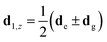
 . We have also defined the transition energy of the Nth site to be ω0 and introduced a site-to-site detuning of Δ, such that an energy gradient can be generated along the chain, with the highest energy at site 1. Here the mixed dipole coupling matrix κijα,β is defined by


 is the phonon displacement operator for the nth dipole, ωn,v, gn,v and b(†)n,v respectively represent the energy, the coupling strength, and the annihilation (creation) operator of the v-mode of the nth dipole's vibrational bath.


 is the effective energy shift of the nth site due to all the other sites permanent dipoles and
  is a constant offset. A simple topological feature emerges: if the permanent-dipole couplings are dominated by nearest-neighbor terms and the dipoles are symmetric, then δn = δn+1 for all non-end sites. Only the first and last sites differ, as they each have a single neighbor, breaking the degeneracy at the chain boundaries by an amount proportional to the permanent dipole strength. We will see below how this boundary effect influences energy transport. The transition dipole–dipole interaction, by contrast, mixes the site basis and enables delocalization, an essential ingredient for transport in the Bloch–Redfield model discussed in the following section.


 where operators Aα and Bα act on the chain system and baths, respectively, we can rewrite the second term on the right-hand side of the Bloch–Redfield master equation as


 . This steady-state current quantifies the number of excitons extracted per unit time when the system is in equilibrium. Whilst the Bloch-Redfield formalism developed here is necessarily a weak-coupling master equation, it can offer powerful explanatory power for qualitatively understanding the dynamics of a large range of systems relevant to energy transport systems.93–95


