DOI:
10.1039/D5SM01005E
(Paper)
Soft Matter, 2025,
21, 9058-9069
A minimal mechanism for flocking in phoretically interacting active particles
Received
1st October 2025
, Accepted 30th October 2025
First published on 3rd November 2025
Abstract
Coherent collective motion is a widely observed phenomenon in active matter systems. Here, we report a flocking transition mechanism in a system of chemically interacting active colloidal particles sustained purely by chemo-repulsive torques at low to medium densities. The basic requirements to maintain the global polar order are excluded volume repulsions and long-ranged repulsive torques. This mechanism requires that the time scale for individual colloids to move a unit length be dominant with respect to the time they deterministically respond to chemical gradients, or equivalently, pair colloids slide together a minimal unit length before deterministically rotating away from each other. Switching on the translational repulsive forces renders the flock a crystalline structure. Furthermore, liquid flocks are observed for a range of chemo-attractive inter-particle forces. Various properties of these two distinct flocking phases are contrasted and discussed. We complement these results with stability analysis of a hydrodynamic model, which reveals the transition corresponding to destabilization of the flocking state observed in particle-based simulations.
I. Introduction
The collective swarming behaviour of interacting agents – also called flocking1 – has been a topic of sustained interest in the field of non-equilibrium statistical physics. Flocking is also a ubiquitous phenomenon in the natural world, widely reported in groups of animals, such as birds, fish, and mammals.2–4 Paradigmatic models that incorporate local alignment interactions to study flocking have been extensively studied1,5–8 and continue to be investigated.9–12 Most notably, in the Vicsek model,5 local alignment interactions among the individual agents can lead to transition from a disordered state to one with large-scale, coordinated movement. The flocking transition in these models with short-range alignment interactions has been widely studied, along with extensive investigation of the nature of the order-to-disorder transition6,8,13,14 and universality of critical exponents.1
The possibility of attaining an emergent global polar order (flocking) arising purely out of dynamical particle-based models, without any explicit alignment interaction, is a subject of recent interest and recently reviewed in ref. 15. Systems where such a phase has been observed are typically over-damped16–18 and include those with velocity alignment interactions,17,19–21 distance-dependent interactions,22 history (trail) dependence23,24 and those with repulsive torques and forces between the particles without volume exclusion.25,26 A separate class of inertial models have also reported such a transition,27–30 including those with attractive interactions.31
Though various possible mechanisms deviating from the Vicsek-like rule have been established, the explicit relevance of the separate contributions of the long-ranged interparticle forces and torques between active particles in producing a global polar order has not been clearly established. For instance, migrating cells that display a global polarity have been known to display chemo-tactic attractive interactions in addition to (among others) either a contact “inhibited” or “attracted” locomotion – akin to a long-ranged torque of either repulsive or attractive nature.18,32,33 Studies on translational and rotational diffusiophoretic motion of active particles (with a self-generated chemical field) with attractive torques indicate collapse of particles into dense clusters.34 In addition, extensive studies on repulsive torques in these systems are rare. Thus, open questions remain on the minimal ingredients and mechanism at play arising from the forces and torques of inter-particle phoretic interactions.
In this paper, we report a minimal mechanism for the formation of liquid flocks, which we herein denote as “chemorepulsive liquid flocks” (CLF). The basic ingredients that are sufficient to produce such a flock are: (i) short-ranged excluded volume repulsive and (ii) long-ranged (chemo) repulsive torques. There is no need for any additional (chemo)repulsive translational forces between the particles, nor is there a requisite role for noise in destabilizing the flock. Furthermore, the incorporation of long-ranged translational chemo-repulsive forces between the particles induces instead crystalline flocks (with regular lattice spacing), which we denote this herein as “chemorepulsive crystalline flocks” (CCF). Our work thus adds insights into investigations on attaining a global polar order via dynamical mechanisms without any explicit alignment interaction, by providing a minimal mechanism, both for flock formation and destabilization, which, to our best knowledge, has not been reported elsewhere.
The remainder of the paper is organized as follows. In Section II, we describe our model to study phoretic (chemical) interactions of active particles and enumerate various important dimensionless parameters of our study. In Section III, we report various simulation results for the CLF, and likewise for the CCF in Section IV. A comparison of these two phases is done in Section V by studying the pair correlation, hexatic order, order-to-disorder transition, density fluctuations and finite-size effects. In Section VI, we demonstrate that flocking persists even for chemo-attractive forces between particles which turn away from each other. Further, we complement the results from particle-based simulation with a stability analysis of a continuum model of coupled density and polarization fields in Section VII. Finally, conclusions and a discussion of our work in relation to other findings are presented in Section VIII.
II. Model
The model consists of two dynamical parts: (a) the dynamics of particles and (b) the dynamics of the chemical concentration field; these are described in the following subsections.
A. Dynamics of the particles
We consider a set of N chemically interacting active colloids of radius b. We model the ith active particle as a colloid particle centered at ri = (xi, yi), confined to move in two-dimensions, which self-propels with a speed v0, along the directions ei = (cos![[thin space (1/6-em)]](https://www.rsc.org/images/entities/char_2009.gif) θi, sinθi). Here i = 1, 2, 3, …, N and θi is the angle made by the orientation ei with respect to the positive x-axis. The orientation ei of the ith particle, given in terms of the angle θi, changes due to coupling its dynamics to the dynamics of a phoretic (scalar) field c, as we describe below. The position ri and orientation ei of the ith particle are given as:
θi, sinθi). Here i = 1, 2, 3, …, N and θi is the angle made by the orientation ei with respect to the positive x-axis. The orientation ei of the ith particle, given in terms of the angle θi, changes due to coupling its dynamics to the dynamics of a phoretic (scalar) field c, as we describe below. The position ri and orientation ei of the ith particle are given as:| | | ṙi = v0ei + χtJi + μFi + ηti, | (1a) |
| | | ėi = χr[(ei × Ji) + ηri] × ei. | (1b) |
Here, v0 is the self-propulsion speed of an isolated active particle. The terms ηti and ηri are white noises with zero mean and no temporal correlation. The variance of noises ηti and ηri is, respectively, 2Dt and 2Dr. These noise terms are included for the sake of completion and to demonstrate that the results are robust against weak fluctuations. The term Ji is chemical flux on the location of the ith particle, which gives the inter-particle interaction (of chemical origin). The phoretic flux is given as: Ji(t) = −[∇c(r,t)]r=ri, where c(r,t) is the concentration of the chemicals (e.g. filled micelles in an oil-emulsion system23,35,36).
The term proportional to χr in eqn (1) drives orientational changes (turning particles away from each other if χr > 0) through interparticle chemical interactions. In this paper, we only consider the case of χr > 0 when particles turn away from each other due to chemical interactions.23,24 Similarly, the term proportional to χt ensures repulsion in the positional dynamics if χt > 0. If both χr and χt are positive, then the system is said to be chemo-repulsive. A schematic representation of the dynamics due to the model is given in Fig. 1 to describe the physical meaning of parameters χr (which controls rotation) and χt (which controls translation) for chemical interactions between the particles.
 |
| | Fig. 1 Schematic description of the chemical interactions between the particles based on eqn (1). The black dot on the orange circles indicates the orientation of the particles. Black curved arrows show rotations from chemical interactions, while solid red arrows show translations from chemical interactions. The particles turn away from each other if χr > 0, while they turn towards each other if χr < 0. Similarly, particles translate away from each other if χt > 0, while they translate towards each other if χt < 0. | |
In eqn (1), to preclude overlap of the particles, there is a short-ranged purely repulsive body force Fi on the particles. The expression of the body force on the ith particle is given as:
| |  | (2) |
With
b as the colloidal radius and
rij = |
ri −
rj|, we choose

to be of the form:
Here,
κ is a constant, which determines the strength of the excluded volume repulsion.
B. Dynamics of the chemical field
Though the focus of this paper is on chemical interactions, we note that our analysis is general and maybe applied to other phoretic fields as well. The chemical concentration field c(r,t) around the particles located at ri is obtained by solving:| |  | (3) |
Here, Dc is the diffusion coefficient and c0 is the emission constant of the chemical. In the above, we have assumed that the chemical interaction between the particles is instantaneous.24,34,37–42 In addition, we assume that each particle is a point source of the chemical field. Finally, the chemical flux Ji on the ith colloid, in the point particle limit, can be written from the solution of eqn (3) as:| |  | (4) |
Here, rij = |rij|, with rij = ri − rj. It is worthwhile to note that in our model, the chemical field diffuses in an infinite three-dimensional half-space, and thus, the chemical field decays as 1/r. Assuming a no-flux boundary condition at the bounding surface, the 1/r dependence of the chemical field remains valid. On the other hand, the particles are confined to move in two-dimensions, such that they move in the plane of the bounding surface. Consequently, the dimensions of chemical concentration are [c] = [L−3] and chemical flux are [J] = [L−4]. So, the dimensions of parameters are [χr] = [L4 T−1] and [χt] = [L5 T−1].
C. Important dimensionless parameters
We note that τ = b/v0 is the propulsion time scale. In addition, we define τr = b4/χr, which sets the time scale for deterministic rotation of the particle due to phoretic interactions. The phenomenology of the CLF can also be understood by studying the dynamics as per the dimensionless numbers of the problem that arise out of the equations of motion (1). They are:| |  | (5) |
Here, Λr is the ratio of propulsion time scale τ and time scale τr which controls rotations of the particle orientations from chemical interactions between particles. On the other hand, Λt is the ratio of translation due to chemical interactions between particles and one-body propulsion. The key parameters of this model are the dimensionless numbers Λr, Λt and ϕ. Here, ϕ is the area fraction. ϕ is related to the number density ρ, as ϕ = (Nπb2)/L2 = ρπb2. The simulation results are henceforth presented as a function of these three parameters.
We note that in principle, there are other relevant dimensionless numbers; e.g. and
and  , which would alter the flocking transition. Our results are presented for effectively noiseless systems; thus, the aforementioned Pe1,2 → ∞. Indeed, the novelty of the mechanism presented here, as we will show below, is its purely deterministic destabilization of the polar phase, independent of any noise contributions.
D. Simulation details
The position and orientations of the particles are updated using a forward Euler–Maruyama method from the dynamical equations given in eqn (1). Initially particles are distributed randomly over the two-dimensional space. The initial orientations are also randomly distributed over the range of angles [−π, +π] (angles are computed with respect to the positive x-axis). Periodic boundary conditions are applied on both the x-axis and y-axis. To compute chemical interactions using the expression of Ji, we need to sum over periodic images. We have used a regular summation convention (using minimum image convention) for all results reported here, and checked these with the full Ewald summation convention for selected parameter values. In this paper, the fluctuations (noise terms) are set to be negligibly small to emphasize that flocks can be formed and destroyed by deterministic causes. Indeed, the polar order is expected to be destroyed at larger values of fluctuations.5 But we do not explore the role of the noise in the positional and rotational sectors in this paper. Instead, we choose their strengths to be sub-dominant compared to deterministic effects due to chemical interactions and self-propulsion. We have taken particle radius b = 1, and the total number of particles varies in the range N = [239, 20000]. The steady-state time averages of the observables are taken over 2 × 10⁵ time steps. The time-stepping of the Euler–Maruyama integrator dt is taken as 0.01. A summary of all of the values of parameters used for the simulation is given in Table 1 in the Appendix.
Table 1 Parameter values used for respective figures of the paper. Here L is the system size, b is the radius of the particle, N is the number of particles, dt is the time-stepping of the Euler–Maruyama integrator. The remaining parameters are defined after eqn (1). We have kept  in all the simulations. Note that we consider noise to be less dominant to deterministic effects. Indeed, for the results in this paper, the Péclet number Pe = v0/(bDr) is around 109
| Figure no. |
L
|
dt |
b
|
v
0
|
κ
|
N
|
ϕ
|
χ
t
|
Λ
t
|
χ
r
|
Λ
r
|
D
r
|
D
t
|
|
Fig. 2
|
100 |
0.01 |
1 |
50 |
175 |
(319, 2578) |
(0.1, 0.8) |
0 |
0 |
(0, 7) |
(0.0, 0.14) |
10−6 |
10−8 |
|
Fig. 3(a)
|
100 |
0.01 |
1 |
50 |
175 |
1024 |
0.32 |
(0, 5) |
(0.0, 0.1) |
(0, 10) |
(0.0, 0.2) |
10−6 |
10−8 |
|
Fig. 4(a) and (c)
|
186 |
0.01 |
1 |
50 |
175 |
4000 |
0.36 |
0 |
0 |
0.75 |
0.015 |
10−6 |
10−8 |
|
Fig. 4(b) and (c)
|
186 |
0.01 |
1 |
50 |
175 |
4000 |
0.36 |
3 |
0.06 |
6 |
0.12 |
10−6 |
10−8 |
|
Fig. 5(a)
|
(77, 354) |
0.01 |
1 |
50 |
175 |
1600 |
(0.04, 0.84) |
0 |
0 |
(0, 9) |
(0, 0.18) |
10−6 |
10−8 |
|
Fig. 5(b)
|
118 |
0.01 |
1 |
50 |
175 |
1600 |
0.36 |
(0, 12) |
(0, 0.6) |
(0, 32) |
(0, 0.64) |
10−6 |
10−8 |
|
Fig. 6(a)
|
100 |
0.01 |
1 |
50 |
175 |
(637, 1592) |
(0.2, 0.5) |
0 |
0 |
(0, 8) |
(0.0, 0.16) |
10−6 |
10−8 |
|
Fig. 6(c)
|
100 |
0.01 |
1 |
50 |
175 |
(637, 1592) |
(0.2, 0.5) |
(0, 10) |
(0.0, 0.2) |
27 |
0.54 |
10−6 |
10−8 |
|
Fig. 7(a)
|
100 |
0.01 |
1 |
50 |
175 |
1024 |
0.32 |
(−1, 0) |
(−0.02, 0.0) |
(0, 10) |
(0.0, 0.2) |
10−6 |
10−8 |
III. CLF via chemo-repulsive torques
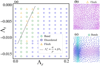
We first consider the case of Λt = 0 (or, equivalently, χt = 0). Thus, repulsions are exclusively short-ranged viaeqn (2) which prevents overlap of particles. First, we vary Λr and ϕ and determine the polar order of the system. The phase diagram delimiting the CLF phases (polar flocks, bands, and disordered states) is shown in Fig. 2(a). The states are delimited via the mean global polarization of the system at the steady state, Pss = 〈|P|〉ss, where the polarization P is defined as the average of sum of the orientation of all the particles:| |  | (6) |
The different phases shown in the phase diagram are distinguished by different values of the magnitude of Pss: flock (Pss > 0.9), bands (0.1 < Pss < 0.9) and disordered (Pss < 0.1). The snapshots of these three phases are presented in Fig. 2(b)–(d) respectively. The dynamics of |P| of the respective cases is shown in Fig. 2(e). On the (ϕ, Λr) plane (Fig. 2(a)), we see that low-density flocks are sustained, which are eventually destabilized at sufficiently high repulsion and densities. These flocks have evidently a liquid-like spatial structure (Fig. 2(b)).25,43,44 The density field ρ is thus not homogeneous across the system (see Fig. 2(b)). Density bands often occur in these systems, where particles move perpendicular to the length of these bands and travel, Fig. 2(c)). For larger systems, many of these dense bands are observed over the space. See Movie I45 for dynamics to obtain CLF starting with a disordered state.
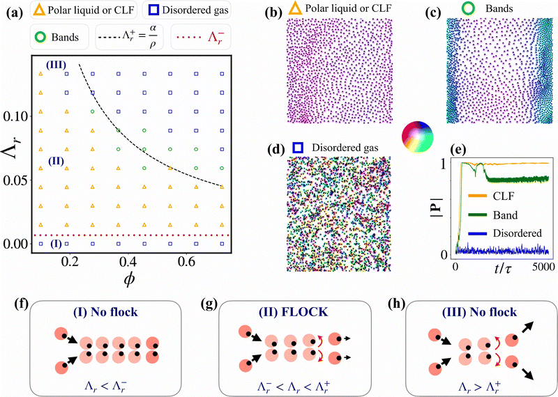 |
| | Fig. 2 CLF for Λt = 0. (a) Phase diagram in the (ϕ, Λr) plane, where ϕ is the area fraction of particles. Here, Λr− is annotated as a dotted red line, while the density dependent Λr+ as a dashed black line. Symbols here and throughout the paper denote a flock (yellow triangle), bands (green circles), and disordered states (blue squares). Marked (I)–(III) scenario and transition lines (black and red) are described in panels (f)–(h). Snapshots of the respective phases are shown in (b)–(d) respectively (color coding for orientation of each particle is in the middle panel). (e) The evolution of the polarization is displayed for the corresponding states (similarly colored). Panels (f)–(h) are a series of scenarios depicted corresponding to parameter choices labelled in panel (a). Scenarios (I) and (III) have chemical response that are either too slow or too quick, such that a stable flock cannot be formed. Panel (g) – scenario (II) – shows the regime in which the chemical response is in an optimal range such that the pair collision mechanism would produce a flock. See Section III A for details of the three distinct cases and mechanism of flocking. | |
A. Mechanism for the formation of CLF
The CLF flock forming region on Fig. 2(a) can be understood by consideration of competing effects between various length (time) scales of the problem. To this end, it is useful to consider the idealization of pair colloidal collision, where the pair collides move along a co-moving frame a distance lsl within a time τsl, whilst rotating away (chemorepulsive). This can be interpreted as a sliding length and time scales respectively, and can be written as:| | 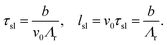 | (7) |
Let us denote Λr− as the smallest value of Λr to sustain the CLF (corresponding to the lowest transition line in Fig. 2a), and Λr+ as the largest value of Λr above which the CLF is not sustained. Λr+ is density dependent, as will be described below. The mechanism for the CLF can then be understood as a competition between Λr and Λr+, Λr−; this is illustrated in Fig. 2(f)–(h) (annotated accordingly in the phase diagram of Fig. 2(a)). From (7), the mechanism can be understood in terms of sliding time scale τsl along with τsl− and τsl+. There are three distinct cases (see the corresponding label on the phase diagram in Fig. 2(a)):
Case I: when Λr < Λr− (corresponding to τsl > τsl−), the orientational changes of the colloids are too slow compared to the free movement time and pair colloids slide excessively long; hence, local polar order cannot be sustained (Fig. 2(f)).
Case II: in the regime of Λr− < Λr < Λr+ (equivalently τsl+ < τsl < τsl−), we have that the chemical response time is fast enough such that local polar order is sustained, but still sufficiently slow such that the forward–backward symmetry at the pair collision level is broken (Fig. 2(g)).
Case III: finally, for Λr > Λr+ (equivalently τsl < τsl+), the chemical response is sufficiently quick such that there is no symmetry breaking at the pair collision level, and hence no local alignment (see Fig. 2(h)).
B. Flocking by sliding an optimal distance while turning away
Using eqn (7), we may also describe the mechanism for CLF in terms of sliding length scale lsl, corresponding to τsl+ and τsl−. These are:
| lsl+ = v0τsl+, lsl− = v0τsl−. |
Note that in this choice of notations, lsl− > lsl+ as the time scale τsl− > τsl+. From simulations at ϕ ≈ 0.31, we find these values to be lsl+ ∼ 8.3b (Λr+ ∼ 0.12) and lsl− ∼ 100b (Λr− ∼ 0.01), and thus for low densities lsl+ of a few times the colloidal radius is feasible, whereas the upper limit spans the box size, which prohibits any flock formation. As we will show (and derive) below, lsl+ is directly proportional to density (with lsl− fixed by the system size), thus CLF formation can be equivalently understood by the competing effects of density-dependent inter-particle (pair) collisions and sliding. We see that the phase boundary in Fig. 2(a) takes the functional form Λr+ = α/ρ. Here, α is a constant that we will later quantify and derive. For densities above a critical density 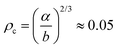 , lsl+ always exceeds the mean free path
  so that flock formation can happen uninhibited. Indeed for very dilute systems (ρ < 0.05, smaller than the densities displayed in Fig. 2), there is no flock formation as there is a large free path movement and thus pair sliding is infrequent (not shown here). For high densities, though pair collisions are more frequent, lsl > lsl+ cannot be satisfied. Indeed, at these densities, lsl+ and lsl− converge and flock formation is prohibited. Thus, for a finite range of densities the CLF can form and stably persist. Equivalently, there is no CLF if the pair colloid slide is too short (lsl < lsl+) or too long (lsl > lsl−).
We clarify at this juncture that such a pair collision mechanism is constructed as an idealization; in actual simulation, pair colloids may not slide an entire lsl before leaving a given collision radius. However, such an abstraction helps us understand the polar alignment mechanism at the pair colloidal level, and in addition agrees fully with simulation results at the collective level. A key feature of this mechanism to be emphasized is the requirement of short-ranged repulsion (provided here via excluded volume interactions), without which CLF formation at χt = 0 would not occur; this instead would have to be supplemented with χt > 0.26 Thus, (i) short-ranged translational repulsion and (ii) long-range orientational torques are the minimal requisite ingredients required for the formation of CLF.
IV. CCF via chemo-repulsive forces and torques
We now switch on χt and ask how the properties of the flock differ. On the (Λr, Λt) plane, we find that there is a clear region of flocking for non-zero χt (see Fig. 3(a)). We further find that the flocks have crystalline order (see Fig. 3(b)). Such crystalline flocks in repulsive systems have been recently reported.26 Similarly to the CLF, the CCF is destabilized by sufficiently high rotational torques. In addition, Λr+ now is linear in Λt. Λr+ is larger for a positive Λt, thus rendering a shorter sliding length for pair colloids during the CCF formation. The net result of a shorter sliding length compared to the CLF is hence attributable to the difference between the crystalline and liquid structures. See Movie II45 for dynamics to obtain CCF starting with a disordered state. We note that if this repulsion is too strong, the CCF is destabilized to a disordered gas (not shown in Fig. 3).
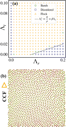 |
| | Fig. 3 (a) Phase diagram in the (Λr, Λt) plane for the case of χt > 0. The dashed line refers to lower bound on χr, the solid line for lower bound on χr from eqn (8). (b) A snapshot of the CCF phase (the same color scheme to indicate the orientation of the particles as in Fig. 2). | |
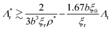
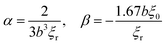
The phase diagrams for the collective dynamics of the system are presented in Fig. 2(a) and 3(a) in terms of the three key dimensionless parameters: Λt, Λr and ϕ. The most generic form of the transition lines from the phase diagrams can be written as:
| |  | (8) |
We obtain
β and
α by first fitting the boundary line in
Fig. 3(a). The slope gives
β ≈ 0.167, whilst the
x-intercept gives
α ≈ 0.013/
b3. This fit is obtained by first applying determining points of greatest variance of the order parameter (susceptibility) on the phase plane and then applying least-squares regression on those points. The fitted
α thus independently fixes the boundary on
Fig. 2(a). The term
α/
ρ inhibits sliding at high densities. The second term due to the presence of long-ranged translational repulsion suppresses the sliding length and contributes to the crystalline structure. The delimiting lines of
Λr− on the left (vertical) of
Fig. 3(a) and bottom (horizontal) of
Fig. 2(a) are equal. Thus, the CCF mechanism may be summarized by being an extension of the CLF mechanism, with the additional long-ranged repulsive forces between the particles rendering the crystalline structure.
V. Differences between CCF and CLF
A. Pair correlation function
The difference in spatial structure between the CLF and CCF is readily distinguished by the pair correlation function, which is given by:| |  | (9) |
This is plotted in Fig. 4(c), distinguishing the solid and liquid signatures.25 A closely related quantity is the polar pair correlation g(r,φ), which explicitly depends on the orientations of the colloids. Here, cos(φij) = ei·![[r with combining circumflex]](https://www.rsc.org/images/entities/b_char_0072_0302.gif) ij, where ij = (rj − rj)/|rj − rj|.46 For the CLF, we see that there are quadrants where neighbours are more likely to be found (Fig. 4(a)), as opposed to the hexatic order of the CCF (Fig. 4(b)). In the case of CCF, the intensity (proportional to the probability of finding the particle from the reference – see Appendix A) in the well-localized hexagonal positions of the crystal is substantially higher than that in the CLF, which are instead less intense with a greater relative spread. The four-lobe distribution is indicative of a highly anisotropic liquid phase where there is a decreased probability of finding a neighboring particle either at the front or back of the reference particle due to mutual repulsion.
ij, where ij = (rj − rj)/|rj − rj|.46 For the CLF, we see that there are quadrants where neighbours are more likely to be found (Fig. 4(a)), as opposed to the hexatic order of the CCF (Fig. 4(b)). In the case of CCF, the intensity (proportional to the probability of finding the particle from the reference – see Appendix A) in the well-localized hexagonal positions of the crystal is substantially higher than that in the CLF, which are instead less intense with a greater relative spread. The four-lobe distribution is indicative of a highly anisotropic liquid phase where there is a decreased probability of finding a neighboring particle either at the front or back of the reference particle due to mutual repulsion.
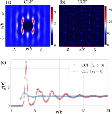 |
| | Fig. 4 Panels (a) and (b) compare g(r,φ) for the case of the CLF and the CCF. In (c), a comparison of the flocking phase, for CLF (red) and CCF (blue), is shown for the pair correlation g(r). | |
B. Hexatic order and density variance
We define a measure of local hexatic order ψi for the ith particle to quantify the hexatic order globally in terms of ψ6. They are given as:47| |  | (10) |
Here, θij is the angle between particle i and particle j and Nni is the number of neighbors for particle i (Nn ≈ 6 for all data points). The observable ψ6 is then averaged over 1000 different particle configurations at the steady-state. We plot ψ6 for the two cases (χt = 0 and χt > 0) in the left panel of Fig. 5. The transition lines from the phase diagrams in Fig. 2(a) and 3(a) are also shown as dotted lines for guiding the eye. In the case of χt = 0 (Fig. 5(a) left), the hexatic order exists in the flocking phase, only for a very high density (area fraction ϕ = ρπb2 > 0.6). On the other hand, in the case of χt > 0 (Fig. 5(b) left), with ϕ = ρπb2 = 0.36, the system becomes highly hexatic in the flocking phase. However, near the transition line, where density bands are prone to occur, we find that the hexatic order gradually decreases.
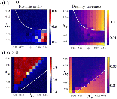 |
| | Fig. 5 Phase diagrams in terms of (left) global hexatic order (ψ6) and (right) density variance. The top panel (a) shows these for the CLF, whereas the bottom panel (b) for the CCF. Dashed curves in each plot indicate the order–disorder (polarization) transition line as in Fig. 2(a) and 3(a). | |
Next, density variance for the two cases (χt = 0 and χt > 0) is shown in the right panel of Fig. 5. The density variance is calculated from the density distribution for a specific parameter set shown in the phase diagram. For local density measurements, the Voronoi tessellation method has been implemented for a spatial configuration of particles. We calculate local density ρl = πb2/Al, where Al is the local area assigned to each particle. Then we compute the density variance as 〈(Δρ)2〉 = 〈ρl2〉 − 〈ρl〉2 (spatial average) and finally averaged over 1000 configurations. In both cases, the density variance is much lower in the flocking state. However, it shows an increase near the transition region. The density variance is high for the high area fraction (ϕ = ρπb2) and in the disordered phase, for the case χt = 0 (Fig. 5(a) right panel). For the χt > 0 case, with low χt values, the variance is more prominent, as shown in Fig. 5(b) (right panel).
C. Phase transition and finite size effects
We now present how polar order parameter |P| changes with variation of the control parameter Λr and Λt, shown in Fig. 6. First, for CLF (Λt = 0), phase transitions are shown for different area fractions ϕ = [0.2, 0.5] with the system of size L = 100 (Fig. 6(a)). With zero Λr, |P| ≈ 0 and there is no flocking (lower bound of Fig. 2(a)). As we increase Λr, particles flock into a polar ordered state. On the other hand, with a further increase in Λr, disordered phases are observed (see Fig. 2(a)). Transition points shift towards lower Λr values with increase of density. Further, we present the finite size effects with different systems of sizes L = [50, 400] (N = [239, 15279]) with a constant area fraction ϕ = 0.3 (Fig. 6(b)). The effects of a finite size on the flocking transition can be clearly seen for systems of smaller size, whereas the effect is minor for a larger system size. Then, for the CCF (with fixed Λr = 0.55), the polar order parameter |P| versus Λt is plotted for different area fractions (for reference, see Fig. 5(b), where the area fraction is fixed at ϕ = 0.36). In Fig. 6(d), we studied finite-size effects for this case and found that the effect on the phase transition is negligible for larger system sizes. It needs to be noted that our model includes long-range interactions, and it is thus computationally expensive to probe sizes beyond those reported here.
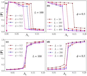 |
| | Fig. 6 Finite-size effects of phase transition. Top panel: (a) shows the magnitude of the polar order parameter |P| versus Λr for the CLF (Λt = 0) for different area fractions ϕ, whilst (b) displays these for different systems of size L. Bottom panel: similarly plotted for the CCF, with the variation with respect to Λt instead for different ϕ (c) and L (d) respectively. Here, we have fixed Λr = 0.55. The total number of particles N corresponding to the L are given as: (L = 50, N = 239), (L = 100, N = 955), (L = 200, N = 3820) and (L = 400, N = 15279). | |
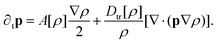
VI. Effect of long-ranged translational chemo-attraction
To further support the robustness of the mechanism, we report flocks arising from repulsive torques with the addition of long-ranged attractive inter-particle forces, thus χt < 0. We find collective motion as flocks are maintained for Λt ∈ [0, −0.01], before transitioning to a disordered state for larger attractive translational interactions; this is shown in Fig. 7(a). In this regime, the clumping tendency is balanced by the excluded volume repulsions. This sets the y-intercept of the theoretical prediction in Fig. 7(a) to be of the same order of magnitude to the lower horizontal line in Fig. 2. These are hence liquid flocks (CLF, see Fig. 7(b)). The band formation is also similar to that of the CLF. During density band formation, often less denser waves form in the system, and they move perpendicular to the direction of the density bands. Similar cross-sea phases are also observed in Vicsek-like models.48
 |
| | Fig. 7 (a) Phase diagram in the (Λr, Λt) plane for the case of χt < 0. The transition line is extrapolated from Fig. 3(a). (b) Liquid flock, (c) density band representing the phases of the phase diagram (the same color scheme as in Fig. 2). Total number of particles N = 1024. | |
VII. Continuum description
To explain the above mechanism, we write top-down hydrodynamic equations for the density ρ(r,t) and polarization p(r,t) fields by appealing to the symmetries and conservation laws of the system.47 The continuum equations for our system can be written as:| | | ∂tρ = −∇·(vtr[ρ]p − Dtr[ρ]∇ρ) | (11a) |
| |  | (11b) |
Here, we have defined:
| vtr[ρ] = v0 − χtξ0ρ, Dtr[ρ] = ξtρχt, |
| A[ρ] = (ξrχr + ξ0χt)ρ − vtr[ρ]. |
The term
vtr (a coarse-grained velocity) appears in both the cross-coupling terms between density and polarization fields, stabilizing the density field at larger
χt. This effect is in turn countered by
Dtr (coarse-grained diffusivity), which randomizes the fields at large
χt. The
χr and
χt contributions
via the
A term act to destabilize the polarization field with respect to density gradients. Given that the transition lines observed are dependent on the area fraction simulated, each of these terms have an explicit density dependence
via the constants
ξ0,
ξt, and
ξr, which are obtained by fitting the transition line predicted by the particle-based simulation in
Fig. 3(a). A route to these equations
via a systematic coarse-grained procedure is well established,
17,46 though it is not pursued in this work. We note that there are no stochastic contributions appearing in the dynamics of the fields
ρ and
p in
eqn (11). We have assumed noise to be negligibly small as explained in the previous section. In effect, the presence of these stochastic terms in the particle-based model is merely necessitated for the formal coarse-graining procedure, but does not play any further role in explaining the instability of the flocking state.
A. Case of χt = 0
First, we may consider the case of only rotational torques. See Fig. 2(a) for phenomenology of this case with χt = 0 from the particle-based model. From (11) – on setting χt = 0 – we obtain an enslaved dynamics of ṗ with respect to the density gradients:| | 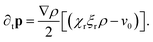 | (12) |
From the above, we see that for the temporal evolution of p to change the nature of stability with respect to the density gradients (feedback response), we require that ρ* is less than:
| |  | (13) |
We see that the fluctuations in both ρ and p are strongly coupled and that any fluctuations are stabilized in the long-time limit.
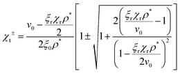
B. General case with χt ≠ 0
For the generic case of both χr ≠ 0 and χt ≠ 0, we may note that solving for ṗ = 0 in (11), whilst ignoring fluctuations, we obtain:
thus generalizing (13) for χt ≠ 0. In the following, we study the stability of the system about these steady-state values for the density field ρ* and a steady-state value of polar order p*.
C. Stability of the flocking state
To study the stability of the flocking state, we linearize eqn (11) for the steady-state density and polarizations (ρ*, p*), defining (δρ, δp) = (ρ − ρ*, p − p*). We use the following choice of Fourier basis expansion| | 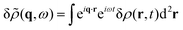 | (14a) |
| | 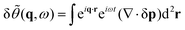 | (14b) |
For a phase with uniform global polarization, the following conditions will hold: ∇ρ* → 0 and ∇·p* → 0.
Eqn (11) can then be linearized on the basis of (14) to obtain the stability condition for the flocking state and subsequently derive the boundary line of eqn (8), for a generic χt. The full linearization in Fourier space yields the following:
| | 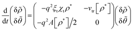 | (15) |
Here
A[
ρ*] = (2
ξ0χt +
ξrχr)
ρ* −
v0. The dispersion relation for
ω(
q) then reads
| | 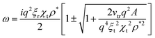 | (16) |
with the condition for linear instability given by:
| 2ξ02ρ*2χt2 − ξ0ρ*(2v0 − ξrχrρ*)χt − v0(ξrχrρ* − v0) < 0 |
Using the above, we can solve for χt. For the value:
| |  | (17) |
we can consider the solution
χt >
χt−. Let us further study the limit

, which corresponds to parameter ranges used in our simulations (see
Table 1).
Using the definitions for Λr and Λt – see eqn (5) – the condition for instability of the modes ω(q) is given by
| |  | (18) |
We can identify this to have the same functional form as
eqn (8) defining the transition line. Equating with
eqn (8), we have that
| |  | (19) |
We can thus infer the values of
ξr ≈ 2/(3
b3α) ≈ 51.3 and
ξ0 ≈ −5.13/
b. The hydrodynamic instability of the flocking phase thus captures the transition lines between ordered and disordered phases in
Fig. 2(a) and 3(a). Though
eqn (18) captures the transition for a generic crystalline flock (generic
χt), we note that there is no explicit spatial-structure instability encoded in the hydrodynamic model,
44 and thus if one simulates
eqn (11) one obtains effectively fluidic flocks at a continuum level. Nevertheless, we conclude that the noiseless limit of a minimal hydrodynamic model captures the destabilization transition of the flock, with exact details of the spatial structure of the system likely requiring to go beyond the conventional molecular chaos hypothesis.
16,17
VIII. Summary and discussion
To conclude, we present a minimal mechanism for formation of fluid flocks that only requires long-ranged (net) repulsive torques and short-ranged repulsive forces from steric interactions. Although the roles of excluded volume interactions,16,20,22,31 repulsive torques – either short22 or long26 ranged – and long-ranged repulsive forces26,31 have been studied separately, we have specified here the individual contributions of each of those components and argued that the former two are the minimal requisite components. The mechanism can summarized as follows: the pair colloids slide together for at least a unit length before deterministically rotating away from each other. This is required to break the forward–backward symmetry at the pair-collision level. Destabilization of the flock arises due to symmetric collisions at the pair colloidal level, wherein they slide exceedingly short before rotating away upon collision. We show that these results are consistent with the noiseless limit of a minimal hydrodynamic theory. One may ask whether such a sliding mechanism alone added to cognitive based (agent based) models13,14 could reproduce the flocking transition; indeed we will leave this to future work.
It is important to note that the CLF and CCF phases are both generated by, and further destabilized by, the deterministic torques themselves, independent of the contribution of noise. Though we have explicit noise terms in the updates in eqn (1) for the sake of completion, they are set to be negligibly small (see Table 1 in the Appendix). We note that we have repeated all the simulations presented in Fig. 2 with Dr = Dt = 0 and have found the results to be identical. Thus, our results on flocking of phoretically interacting active particles and their destabilization are distinct from conventional picture of noise-induced inhibition of flock formation.6,13,26,31 We note that in the absence of short-ranged excluded volume repulsions, our results on the formation of CLF would converge to that recently studied in ref. 26 where the need for (long-ranged) repulsive forces is more imminent. Translational repulsion merely renders the flock to acquire a crystalline structure. We also find flocks for (a narrow range of) long-ranged attractive forces, if of the order of less than the short-ranged repulsion. We have not studied here the role of particle shape anisotropy,17,49 which would add additional competing length scales to our analysis. We have also not studied the role of hydrodynamic interactions between the particles.3,50,51 We expect our results here to be directly relevant to a variety of experimental systems. For example, migrating cell collections have been widely reported to exhibit spatial organization resembling a polar fluid,18,33 while their interaction mechanism has been known to include (among others) long-ranged chemotaxis and avoidance torques.32 The presented mechanism being very generic, we expect it to also be relevant for interacting colloids with non-diffusiophoretic fields,25,44,46 where the underlying mechanism should also hold.
Conflicts of interest
There are no conflicts to declare.
Data availability
Supplementary information (SI) is available. See DOI: https://doi.org/10.1039/d5sm01005e.
The datasets are generated from simulation. They are available from the corresponding authors upon reasonable request.
Appendices
1. Table of parameters
A table of all the parameters used for the generated figures is presented in Table 1.
A Pair correlation functions
The pair distribution function g(r,φ,θ) implies correlations and provides the probability density of finding a pair of particles at a distance r with self-propulsion angle θ. Here, φ is the angle between the relative position r and the self-propulsion direction of the tagged particle, êi·ij = cosφ and θ is the angle between the propulsion directions of the particle pair. To obtain this pair distribution function, histograms are created with the number of particles Nh(r,φ,θ) at distance r, positional angle φ and angle θ. The bins are chosen as 0.1b for r, π/150 for φ and π/2 for θ. Then we need to normalize Nh(r,φ,θ), to obtain the pair distribution function g(r,φ,θ). The number of configurations is tc (10000 snapshots), over which histograms are made. The area of the annular segment of radial width dr and angular width dφ is given by Ar = rdrdφ. The number density is ρ = N/L2 and the size of the relative orientation bin is dθ. Then the normalization factor is  and the pair distribution function is given by g(r,φ,θ) = Nh(r,φ,θ)/Nr.
An example of this for the isotropic phase is given in Fig. 8(a). The pair distribution functions are determined for the four different θ ranges as: θ: [0, π/2], θ: [π/2, π], θ: [−π, −π/2] and θ: [−π/2, 0]. We see that in the isotropic phase, the probability of finding a neighboring particle is different in the front relative to the back of the direction of motion (orientation), indicative of the symmetry breaking in an active disordered gas.17,26,46 In the main text, we show that g(r,φ) also distinguishes CLFs from CCFs, the former having a four-lobe structure compared to the latter's hexatic structure. In addition, we compare the structure of g(r,φ) for the band phases in Fig. 8(b), for the CLF and CCF density bands. We see that the CLF and CCF bands are distinguished strongly via this measure: in the former there is a strong likelihood of finding neighbouring colloids in either the front or back of the propulsion direction, whilst in the latter the aggregate structure resembles that of a (non-polar) liquid due to the presence of cross bands. Note that the band structure is more dense in the case of χt = 0, resulting in a more intense correlation in g(r,φ). A related quantity that we compute is the radial g(r). This is plotted in Fig. 4, distinguishing the CLF and CCF.
 |
| | Fig. 8 Pair correlation function g(r,φ,θ) for the isotropic phase for four different θ ranges in panel (a). In panel (b), we show pair correlation function g(r,φ) in the band phase for χt = 0 and χt > 0. | |
B Description of the supplementary movies
The time evolution of the CCF and CLF structures for a larger system with the total number of particles N = 20000, is attached as supplementary movies.45 We note that our results are robust as we change the number of particles in the simulations. For both cases, we started with random initial conditions (positions and orientations) and updated the equation of motion following eqn (1). In both movies, the particles are colored by their orientations (given in terms of the angle θ their orientation vector makes with the positive x-axis). The color bar is the same as the one used in Fig. 2. Two particles are intentionally colored black throughout the simulation to simply trace them during the dynamics. Polar order or the flocking state collectively emerges in this model with both the cases. Parameters used for the two movies are below.
• Movie I: in the case of χt = 0 (CLF), the liquid flock gradually forms throughout the system and moves in a particular direction. The fixed parameter values are: L = 418, b = 1, dt = 0.01, Dr = 10−3, Dt = 10−3, κ = 175, v0 = 50, χt = 0, χr = 0.75.
• Movie II: in the case of χt > 0 (CCF), the particles first start to form local polar flocks (colored patch), then merge and pick a particular direction of motion entirely. The fixed parameter values are: L = 418, b = 1, dt = 0.01, Dr = 10−3, Dt = 10−3, κ = 175, v0 = 50, χt = 3, χr = 6.
• Movie III: in the case of χt = 0 (CLF), particles form several density bands throughout the space. Additionally, less dense waves (which move perpendicular to the direction of density bands) are also seen to form with these density bands. The fixed parameter values are: L = 418, b = 1, dt = 0.01, Dr = 10−3, Dt = 10−3, κ = 175, v0 = 50, χt = 0, χr = 2.0.
Acknowledgements
We thank Professor Mike Cates for discussions. We also extend our gratitude to two anonymous reviewers of the manuscript for their feedback and constructive criticism, which led to an improvement in the presentation of our results. AGS acknowledges funding from the DIA Fellowship from the Government of India. SA acknowledges support from the National Postdoctoral Fellowship (SERB File number: PDF/2023/002096) provided by ANRF, Government of India. RS acknowledges support from seed and initiation grants from IIT Madras as well as a Start-up Research Grant from SERB (SERB File Number: SRG/2022/000682), India.
References
-
J. Toner, The Physics of Flocking: Birth, Death, and Flight in Active Matter, Cambridge University Press, 2024 Search PubMed.
- I. D. Couzin, J. Krause, R. James, G. D. Ruxton and N. R. Franks, Collective memory and spatial sorting in animal groups, J. Theor. Biol., 2002, 218, 1 CrossRef PubMed.
- M. C. Marchetti, J.-F. Joanny, S. Ramaswamy, T. B. Liverpool, J. Prost, M. Rao and R. A. Simha, Hydrodynamics of soft active matter, Rev. Mod. Phys., 2013, 85, 1143 CrossRef CAS.
- T. Vicsek and A. Zafeiris, Collective motion, Phys. Rep., 2012, 517, 71 CrossRef.
- T. Vicsek, A. Czirók, E. Ben-Jacob, I. Cohen and O. Shochet, Novel type of phase transition in a system of self-driven particles, Phys. Rev. Lett., 1995, 75, 1226 CrossRef CAS PubMed.
- H. Chaté, F. Ginelli, G. Grégoire and F. Raynaud, Collective motion of self-propelled particles interacting without cohesion, Phys. Rev. E:Stat., Nonlinear, Soft Matter Phys., 2008, 77, 046113 CrossRef PubMed.
- S. Mishra, A. Baskaran and M. C. Marchetti, Fluctuations and pattern formation in self-propelled particles, Phys. Rev. E:Stat., Nonlinear, Soft Matter Phys., 2010, 81, 061916 CrossRef PubMed.
- J. Toner, Y. Tu and S. Ramaswamy, Hydrodynamics and phases of flocks, Ann. Phys., 2005, 318, 170 CAS.
- J. Toner, Birth, death, and horizontal flight: Malthusian flocks with an easy plane in three dimensions, Phys. Rev. E, 2024, 110, 064604 CrossRef CAS PubMed.
- H. Ikeda, Minimum scaling model and exact exponents for the nambu-goldstone modes in the vicsek model, Phys. Rev. Lett., 2024, 133, 258301 CrossRef CAS.
- H. Chaté and A. Solon, Dynamic scaling of two-dimensional polar flocks, Phys. Rev. Lett., 2024, 132, 268302 CrossRef.
- P. Jentsch and C. F. Lee, New universality class describes vicsek's flocking phase in physical dimensions, Phys. Rev. Lett., 2024, 133, 128301 CrossRef CAS PubMed.
- S. Adhikary and S. Santra, Pattern formation and phase transition in the collective dynamics of a binary mixture of polar self-propelled particles, Phys. Rev. E, 2022, 105, 064612 CrossRef CAS PubMed.
-
S. Adhikary and S. Santra, Collective dynamics and phase transition of active matter in presence of orientation adapters, arXiv, 2023, preprint, arXiv:2302.13035 DOI:10.48550/arXiv.2302.13035.
- P. Baconnier, O. Dauchot, V. Démery, G. Düring, S. Henkes, C. Huepe and A. Shee, Self-aligning polar active matter, Rev. Mod. Phys., 2025, 97, 015007 CrossRef.
-
L. Chen, K. J. Welch, P. Leishangthem, D. Ghosh, B. Zhang, T.-P. Sun, J. Klukas, Z. Tu, X. Cheng and X. Xu, Molecular chaos in dense active systems, arXiv, 2023, preprint, arXiv:2302.10525 DOI:10.48550/arXiv.2302.10525.
- R. Großmann, I. S. Aranson and F. Peruani, A particle-field approach bridges phase separation and collective motion in active matter, Nat. Commun., 2020, 11, 5365 CrossRef.
- T. Hiraiwa, Dynamic self-organization of idealized migrating cells by contact communication, Phys. Rev. Lett., 2020, 125, 268104 CrossRef CAS PubMed.
- J. Chen, X. Lei, Y. Xiang, M. Duan, X. Peng and H. Zhang, Emergent chirality and hyperuniformity in an active mixture with nonreciprocal interactions, Phys. Rev. Lett., 2024, 132, 118301 CrossRef CAS.
- A. Martn-Gómez, D. Levis, A. Daz-Guilera and I. Pagonabarraga, Collective motion of active brownian particles with polar alignment, Soft Matter, 2018, 14, 2610 RSC.
- E. Sese-Sansa, I. Pagonabarraga and D. Levis, Velocity alignment promotes motility-induced phase separation, Europhys. Lett., 2018, 124, 30004 CrossRef.
- M. Knežević, T. Welker and H. Stark, Collective motion of active particles exhibiting non-reciprocal orientational interactions, Sci. Rep., 2022, 12, 19437 CrossRef PubMed.
- M. Kumar, A. Murali, A. G. Subramaniam, R. Singh and S. Thutupalli, Emergent dynamics due to chemo-hydrodynamic self-interactions in active polymers, Nat. Commun., 2024, 15, 4903 CrossRef CAS PubMed.
- A. G. Subramaniam, M. Kumar, S. Thutupalli and R. Singh, Rigid flocks, undulatory gaits, and chiral foldamers in a chemically active polymer, New J. Phys., 2024, 26, 083009 CrossRef.
- A. Bricard, J.-B. Caussin, N. Desreumaux, O. Dauchot and D. Bartolo, Emergence of macroscopic directed motion in populations of motile colloids, Nature, 2013, 503, 95 CrossRef CAS PubMed.
- S. Das, M. Ciarchi, Z. Zhou, J. Yan, J. Zhang and R. Alert, Flocking by turning away, Phys. Rev. X, 2024, 14, 031008 CAS.
- D. Grossman, I. Aranson and E. B. Jacob, Emergence of agent swarm migration and vortex formation through inelastic collisions, New J. Phys., 2008, 10, 023036 CrossRef.
- T. Hanke, C. A. Weber and E. Frey, Understanding collective dynamics of soft active colloids by binary scattering, Phys. Rev. E:Stat., Nonlinear, Soft Matter Phys., 2013, 88, 052309 CrossRef PubMed.
- K.-D. N. T. Lam, M. Schindler and O. Dauchot, Self-propelled hard disks: implicit alignment and transition to collective motion, New J. Phys., 2015, 17, 113056 CrossRef.
- J. P. Miranda, D. Levis and C. Valeriani, Collective motion of energy depot active disks, Soft Matter, 2025, 21, 1045 RSC.
- L. Caprini and H. Löwen, Flocking without alignment interactions in attractive active brownian particles, Phys. Rev. Lett., 2023, 130, 148202 CrossRef CAS PubMed.
- B. A. Camley and W.-J. Rappel, Physical models of collective cell motility: from cell to tissue, J. Phys. D:Appl. Phys., 2017, 50, 113002 CrossRef PubMed.
- M. Hayakawa, T. Hiraiwa, Y. Wada, H. Kuwayama and T. Shibata, Polar pattern formation induced by contact following locomotion in a multicellular system, eLife, 2020, 9, e53609 CrossRef PubMed.
- O. Pohl and H. Stark, Dynamic clustering and chemotactic collapse of self-phoretic active particles, Phys. Rev. Lett., 2014, 112, 238303 CrossRef PubMed.
- B. V. Hokmabad, J. Agudo-Canalejo, S. Saha, R. Golestanian and C. C. Maass, Chemotactic self-caging in active emulsions, Proc. Natl. Acad. Sci. U. S. A., 2022, 119, e2122269119 CrossRef CAS PubMed.
- P. Dwivedi, D. Pillai and R. Mangal, Self-propelled swimming droplets, Curr. Opin. Colloid Interface Sci., 2022, 61, 101614 CrossRef CAS.
- B. Liebchen and H. Löwen, Which interactions dominate in active colloids?, J. Chem. Phys., 2019, 150, 061102 CrossRef.
- S. Saha, R. Golestanian and S. Ramaswamy, Clusters, asters, and collective oscillations in chemotactic colloids, Phys. Rev. E:Stat., Nonlinear, Soft Matter Phys., 2014, 89, 062316 CrossRef PubMed.
- R. Soto and R. Golestanian, Self-assembly of active colloidal molecules with dynamic function, Phys. Rev. E:Stat., Nonlinear, Soft Matter Phys., 2015, 91, 052304 CrossRef PubMed.
- G. Rückner and R. Kapral, Chemically powered nanodimers, Phys. Rev. Lett., 2007, 98, 150603 CrossRef PubMed.
- R. Singh, R. Adhikari and M. Cates, Competing chemical and hydrodynamic interactions in autophoretic colloidal suspensions, J. Chem. Phys., 2019, 151, 044901 CrossRef.
- G. Turk, R. Adhikari and R. Singh, Fluctuating hydrodynamics of an autophoretic particle near a permeable interface, J. Fluid Mech., 2024, 998, A34 CrossRef CAS.
- D. Geyer, A. Morin and D. Bartolo, Sounds and hydrodynamics of polar active fluids, Nat. Mater., 2018, 17, 789 CrossRef CAS PubMed.
- D. Geyer, D. Martin, J. Tailleur and D. Bartolo, Freezing a flock: Motility-induced phase separation in polar active liquids, Phys. Rev. X, 2019, 9, 031043 CAS.
- See the SI at this URL: [https://doi.org/10.1039/d5sm01005e].
- J. Zhang, R. Alert, J. Yan, N. S. Wingreen and S. Granick, Active phase separation by turning towards regions of higher density, Nat. Phys., 2021, 17, 961 Search PubMed.
-
P. M. Chaikin, T. C. Lubensky and T. A. Witten, Principles of condensed matter physics, Cambridge University Press, Cambridge, 1995, vol. 10 Search PubMed.
- R. Kürsten and T. Ihle, Dry active matter exhibits a self-organized cross sea phase, Phys. Rev. Lett., 2020, 125, 188003 CrossRef.
- H. Wensink and H. Löwen, Emergent states in dense systems of active rods: from swarming to turbulence, J. Phys.:Condens. Matter, 2012, 24, 464130 CrossRef CAS PubMed.
- R. Aditi Simha and S. Ramaswamy, Hydrodynamic fluctuations and instabilities in ordered suspensions of self-propelled particles, Phys. Rev. Lett., 2002, 89, 058101 CrossRef CAS.
- S. Thutupalli, D. Geyer, R. Singh, R. Adhikari and H. A. Stone, Flow-induced phase separation of active particles is controlled by boundary conditions, Proc. Natl. Acad. Sci. U. S. A., 2018, 115, 5403 CrossRef CAS.
Footnote |
| † Contributed equally. |
|
| This journal is © The Royal Society of Chemistry 2025 |
Click here to see how this site uses Cookies. View our privacy policy here. 
 and
Rajesh
Singh
and
Rajesh
Singh


 to be of the form:


 and
and  , which would alter the flocking transition. Our results are presented for effectively noiseless systems; thus, the aforementioned Pe1,2 → ∞. Indeed, the novelty of the mechanism presented here, as we will show below, is its purely deterministic destabilization of the polar phase, independent of any noise contributions.
 in all the simulations. Note that we consider noise to be less dominant to deterministic effects. Indeed, for the results in this paper, the Péclet number Pe = v0/(bDr) is around 109


 , lsl+ always exceeds the mean free path
  so that flock formation can happen uninhibited. Indeed for very dilute systems (ρ < 0.05, smaller than the densities displayed in Fig. 2), there is no flock formation as there is a large free path movement and thus pair sliding is infrequent (not shown here). For high densities, though pair collisions are more frequent, lsl > lsl+ cannot be satisfied. Indeed, at these densities, lsl+ and lsl− converge and flock formation is prohibited. Thus, for a finite range of densities the CLF can form and stably persist. Equivalently, there is no CLF if the pair colloid slide is too short (lsl < lsl+) or too long (lsl > lsl−).


 , which corresponds to parameter ranges used in our simulations (see Table 1).


 and the pair distribution function is given by g(r,φ,θ) = Nh(r,φ,θ)/Nr.
