Oscillatory flow improves hydrodynamic ordering of soft suspensions in rectangular channels

Abstract

A computational study is presented that examines the hydrodynamic ordering of soft-particle suspensions within rectangular channels undergoing both steady and oscillatory flow. In these conditions, particles assemble into one-dimensional train-like configurations aligned in the flow direction. The results indicate that oscillatory flow facilitates a significant improvement in the ordering process, particularly for the assembly of multiple side-by-side trains within the channel. Several key parameters are systematically varied, including the Wolmersley number (Wo) representing the oscillatory frequency, the capillary number (Ca) representing the particle deformability, and the particle volume fraction (ϕ). It is found that optimal ordering occurs for a particular range of Wo number, and that this range is dependent on Ca. Finally, polydisperse suspensions are also considered, whereby dispersity in the particle size is varied. The simulations reveal that oscillatory flow is more robust (relative to steady flow) for ordering polydisperse suspensions into side-by-side train structures. This study provides an alternative strategy for reliably ordering biological cells, vesicles, droplets, or other deformable particles into train-like configurations without the use of flow-focusing fluidic channel features.

---

1. Introduction

Significant hydrodynamic interactions can arise in particle suspensions flowing within closed channels, particularly when the cross-sectional dimensions of the channel are less than ∼100a (a representing the particle radius). The hydrodynamic interactions arise from the flow disturbances that occur due to the relative motion of each particle with respect to the surrounding fluid. These flow disturbances are altered in complex ways due to many factors including the presence of other particles, the presence of the walls, the inertia of the fluid, the deformability of the particles, and the cross-sectional dimensions of the channel.

In certain combinations of the above parameters, the hydrodynamic interactions can lead to collective ordering of the particles. For the case of rigid particles, collective ordering only occurs at moderate-to-high values of Reynolds number (Re).^1–7 In cylindrical channels, rigid particles have been observed to assemble into trains with uniform axial spacings along the flow direction.¹ The trains are located at the Segré–Silberberg annulus, or roughly 0.6R depending on the flowrate (R being the channel radius). In rectangular channels, the channel size and aspect ratio strongly influence the train location and arrangement.^4,5,8 For channels of larger widths (greater than ∼10a), single-file trains form near the wall centers (particularly the wall of greater length). However, if the channel width is small enough (less than ∼10a), staggered particle trains develop with particles residing on alternating locations on either side of the channel. The spacing between particles in trains is most strongly governed by the particle Reynolds number.⁹ The underlying mechanism of this train assembly is a confinement-induced reversing flow field near the sidewalls.⁴ However, it is important to point out that in these rigid-particle suspensions, not all particles belong to trains (the ordering is not very consistent), and defects are common.

On the other hand, deformable particles exhibit a much higher propensity for collective ordering in confined flow.^10–17 Janssen et al.¹² demonstrated that suspended droplets flowing between two infinite parallel plates assemble into 1D trains aligned in the flow direction (the plates separated by 2.4a). They showed that the hydrodynamic interactions arise from the combination of dipolar and quadrupolar flow disturbance fields, the latter caused by the flow-induced deformation of the droplets. It appears that these aligning interactions are universal to particle type (droplet, red blood cell, vesicle, capsule, etc.), given that the particles are soft enough to undergo flow-induced deformation, with a sufficient degree of confinement. For example, experimental studies have shown that red blood cells also assemble into 1D train structures in Poiseuille flow conditions.^18,19 In a recent paper by the current author,²⁰ a parametric study using computer simulations was performed for elastic fluid-filled capsules flowing between infinite parallel plates. An assessment of how the degree of ordering is dependent on the particle deformability, the channel height, as well as the polydispersity of the particles (including dispersity in both size and deformability) was made. In particular, it was found that an optimal channel height of h/a ∼ 5/3 (h representing the half-height of the channel) exists for ordering, when the particle volume fraction is fixed at 10%. This optimality of h/a exists due to a balance between two factors as h/a is decreased: (1) the increasing hydrodynamic interactions that occur with increasing confinement, and (2) the decreasing planar density of particles on the channel half-plane when the particle volume fraction is held fixed. However, even with optimal conditions for ordering, the particle configurations still contained defects in the form of train splitting and merging (i.e. dislocations) as well as some misaligned particles.

Due to the fact that this ordering is a time-dependent process, it requires extended channel lengths on the order of 10³–10⁴a. Incorporating such channel lengths in a microfluidic device can complicate the design layout, as well as incur a substantial energy cost to produce the necessary pressure difference to drive flow (also a concern when increasing Re in inertial microfluidic devices). One strategy to circumvent these challenges is to use unsteady pulsatile flows,²¹ in which a transient pressure difference is applied across the channel. Very recent studies have demonstrated that unsteady harmonic flows can be tremendously effective in reducing clogging, enhancing mixing and particle separation, and improving microdroplet pinch-off and control.^22–28 The special case of oscillatory flow (i.e. zero mean flow rate) is particularly intriguing due to the potential to achieve a desired flow-induced particle distribution in arbitrarily short channels. It has been shown that for rigid particles in dilute concentrations, oscillatory flow alters the inertial focusing in a complex manner that depends on particle inertia and the oscillatory frequency.^29–31 For deformable particles in dilute concentrations, the rate of inertial focusing can be accelerated with certain pulsatile flow frequencies.^32,33

However, the effect of unsteady flows on hydrodynamic ordering in confined soft suspensions is unknown. Here, three-dimensional simulations are presented that demonstrate that oscillatory flow facilitates a significant improvement in hydrodynamic ordering of soft particles in rectangular channels, relative to steady flow conditions. It is found that certain ranges of oscillatory flow frequency are optimal for ordering an initially random suspension into one with multiple side-by-side train structures aligned in the flow direction. This study also compares ordering between steady and oscillatory flows with varying particle volume fraction. At low particle volume fractions, it is found that both oscillatory and steady flow conditions can order a suspension into a single train located at the channel centerline. However, at higher volume fractions, only oscillatory flow was observed to be capable of ordering a suspension into multiple side-by-side trains. Lastly, it is found that oscillatory flow, compared with steady flow, is more robust at ordering suspensions with polydispersity in particle size.

2. Methods

In this study, the immersed boundary method (IBM), coupled with the lattice-Boltzmann method (LBM), is used to simulate a suspension of soft particles flowing through confined rectangular channels. A full description of the model can be found in recent papers by this author,^20,34 however the pertinent details are given below.

The soft particles are fluid-filled capsules with an infinitesimally thin hyperelastic membrane. The membrane is discretized into a triangular mesh with 1280 faces and 642 nodes by subdividing the faces of an icosahedron and projecting the nodes onto a sphere with radius a, corresponding to the resting radius of a capsule. The fluid inside the capsule is assumed to have the same viscosity and density as that of the outside fluid. The Skalak model³⁵ is used to describe the in-plane shear and area-dilation deformation energy of the membrane, with κ_s and κ_a representing the shear and area-dilation moduli, respectively. An out-of-plane bending energy model and a volume conservation model are included as well, as described in ref. 34.

The LBM discretizes the flow field with a uniform, three-dimensional lattice (here, the D3Q19 stencil is used) on which discrete particle distribution functions f_i(x,t) are stored and updated through time. As shown in Fig. 1a, the direction of flow is aligned with the x-axis, and it is driven by a uniform body force density, F^b_x, which is equivalent to a pressure gradient Δp in the flow direction. Channel walls are perpendicular to the y- and z-directions, which are modeled as no-slip surfaces using half-way bounce-back boundary conditions.³⁶ The cross-sectional dimensions of the channel are defined by w and h corresponding to the half-width and half-height of the channel, respectively. The number of lattice sites used in the LBM to discretize the channel is N_x × N_y × N_z (with N_y = 2w and N_z = 2h). In the simulations below, two lattice dimensions are considered: 1000 × 66 × 18 and 1000 × 88 × 18. The spacing between adjacent lattice sites is designated by Δx and is equal in each direction. The time step size is designated by Δt. As is customary, the LBM simulations utilize reduced length and time scales with Δx = 1 and Δt = 1. The fluid density is ρ = 1 and the fluid kinematic viscosity is ν = c_s²(τ − Δt/2) = 1/6, assuming is the lattice speed of sound and the relaxation time τ = 1. In addition, the channel cross-sectional width and height are non-dimensionalized by dividing by the resting particle radius (w/a and h/a). Here, a = 6Δx, so the two channel widths considered in this study are w/a = 5.5 and w/a = 7.33. The channel height is fixed at h/a = 1.5 for all simulations.

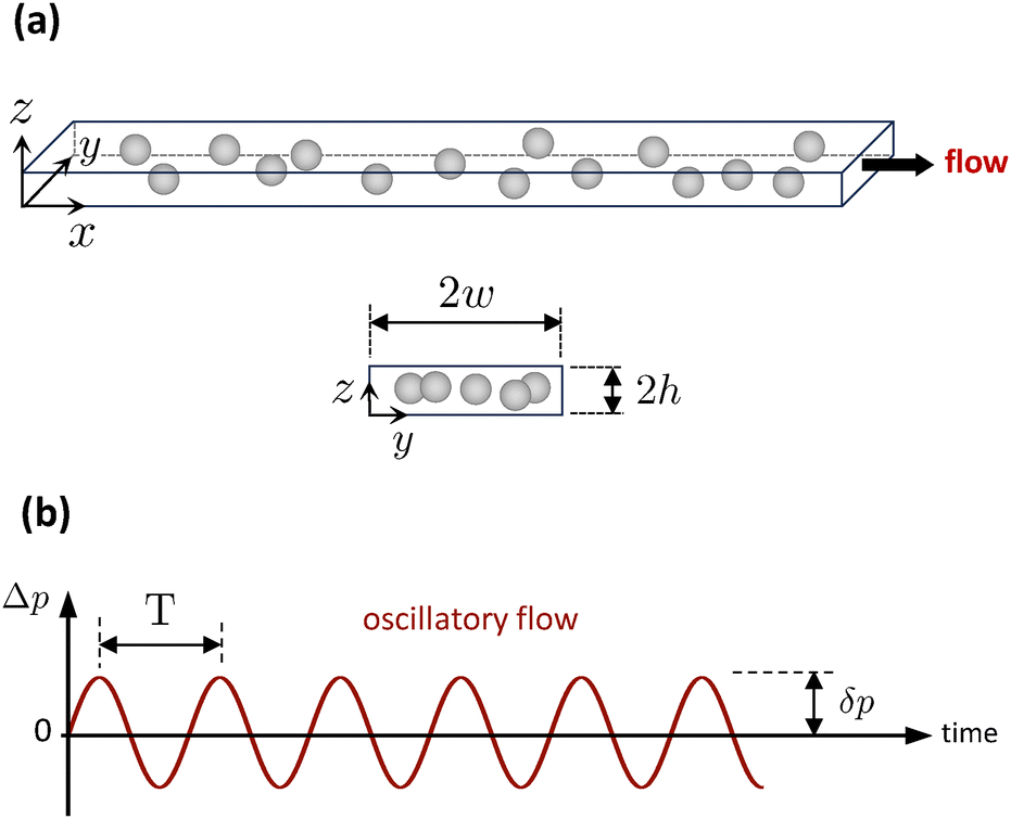Fig. 1 (a) Schematic of simulation domain. The cross-sectional channel dimensions are 2w × 2h, and flow is in the x-direction. (b) Oscillatory flow is realized using a harmonic pressure gradient Δp (equivalent to the body force density F^b_x) in the x-direction with an amplitude δp and time period T. For all oscillatory flow simulations herein, the δp value is chosen such that Re_max = ±1.

The key dimensionless parameters in this study are the Reynolds number (Re) defining the flow inertia in the channel, the capillary number (Ca) defining the particle deformability, and the Wolmersley number (Wo) defining the oscillatory flow frequency. The Reynolds number is defined as:²⁰

where u_max is the maximum velocity in the channel centerline, L is a characteristic length scale set equal to D_h/2 where D_h is the hydraulic diameter of the rectangular channel, and ν is the kinematic viscosity of the bare fluid. It is noted that Re is the channel Reynolds number for the bare fluid (rather than the effective Re of the suspension). For a given value of Re, the x-direction body force F^b_x can be calculated using the analytical solution for u_max given in Appendix A of the author's previous work (see eqn (A6) in ref. 34). The capillary number is defined as:²⁰where ρ is the fluid density and κ_s is the in-plane shear modulus of the particle membrane. For a given value of Ca, the membrane shear modulus κ_s can be calculated directly using eqn (2).

In simulations with oscillatory flow, the body force applied to the fluid is multiplied by a time-dependent sinusoidal function: F^b_x = F̄^b_xsin(2πt/T) = F̄^b_xsin(ωt), where t is simulation time and F̄^b_x, T and ω define the amplitude, oscillation period, and angular frequency of one oscillatory cycle, respectively. Note that the amplitude F̄^b_x is equivalent to δp shown in Fig. 1b. In all simulations herein, the amplitude of the body force density is chosen such that Re_max = ±1. The Wolmersley number is defined as:²¹

Finally, the particle volume fraction is defined as ϕ = NV_p/V_c × 100% where N is the number of particles in the channel, V_p is the volume of one particle (with a spherical shape at rest with a = 6Δx), and V_c is the volume of the channel.

Each simulation begins with a random distribution of particles within the channel. As time progresses, the hydrodynamic interactions due to both the confinement and flow-induced particle deformation lead to the ordering of particles into 1D train assemblies. Two dimensionless order parameters are utilized to characterize the degree of order in the system, and its dependency on the flow and particle properties. The first order parameter Φ_t represents the fraction of particles belonging to a train. The criteria for determining if a particle belongs to a train is the same as the author's recent work.²⁰ Briefly, a particle belongs to a train if it has two neighbors (one in front and one in back) that are within a cutoff radius of 3.5a and within an angular range of ±15° relative to the flow direction. Additionally, a particle belongs to a train if it has one neighboring particle in this same relative position and that neighbor belongs to a train (this second criteria accounts for particles at the head or tail of a train). A train consists of three or more particles. Fig. 2 shows an example simulation whereby capsules are colored according to the train in which they reside.

Fig. 2 Throughout each simulation, particle positions are analyzed to determine which particles belong to a train. Top-down views are shown (of the xy-plane) of both the initial state and the final state at the end of the simulation with steady flow and particle volume fraction of ϕ = 7.62%. In the bottom image, particles in the same train are assigned the same unique color. In this figure, particles not in a train are colored light-grey, as indicated in the close-up view on the right (corresponding to the region circled by the dashed red line).

A second order parameter is introduced here which represents the average train length in the suspension relative to the channel length. The length of any particular train is calculated by summing the distance between sequential neighboring particles in the same train beginning at the tail of the train. Compared to Φ_t, provides a much more sensitive calibration of the train development. When , the average train length is zero (and, hence, there are no trains in the channel). When , every train in the channel extends across the entire channel length. Recall that the domain is periodic in the flow direction (the x-direction), therefore when each train wraps around back onto itself, effectively making its length infinite.

As discussed above, two channel cross sectional dimensions are considered: (i) w/a = 5.5, h/a = 1.5, and (ii) w/a = 7.33, h/a = 1.5. This channel height h/a closely corresponds to the optimal confinement for particle ordering.²⁰ The channel widths are comparable to those used by Iss et al.¹⁹ for red blood cell ordering. For channel widths of w/a = 5.5, each simulation is run for 2 × 10⁶ LBM time steps. For the slightly wider channel widths of w/a = 7.33, each simulation is run for 3 × 10⁶ LBM time steps. Time is non-dimensionalized by dividing by the advection time, defined as the time required for a particle at the channel centerline to travel a distance a:

For steady-flow conditions, u_max is constant and for Re = 1, w/a = 5.5, and h/a = 1.5 corresponds to a value of u_max = 0.0118 Δx/Δt in LBM units. For the wider channels (w/a = 7.33), u_max = 0.0112 Δx/Δt in LBM units. For oscillatory flows, eqn (4) uses u_max at the peak of a cycle, and because Re_max = ±1, the u_max values given above remain valid.

3. Results

3.1. Steady flows

Before results of oscillatory flow are examined, it is important to understand the hydrodynamic ordering behavior in steady flow conditions. As discussed in the Introduction, given sufficient particle deformability and confinement, soft-particle suspensions in planar or rectangular Poiseuille flow conditions undergo an ordering process into 1D train assemblies due to long-range quadrupolar interactions. Recent studies^19,20 have demonstrated that these interactions depend on Re, Ca, ϕ, and the cross-sectional dimensions of the channel.

Fig. 3 provides simulation snapshots that demonstrate the flow-induced ordering for steady flow with Re = 1, Ca = 0.3, and cross-sectional dimensions w/a = 5.5 and h/a = 1.5. The top two rows show a suspension with ϕ = 4.19%, including the initial state (Fig. 3a) consisting of randomly dispersed particles and the flow-assembled state (Fig. 3b) in which all the particles have assembled into a single-file train at the channel centerline. Both top-down views (viewed along the z-axis) and head-on views (viewed along the x-axis) are provided. The pairwise interactions for this flow condition include both long-range attraction and short-range repulsion forces, and therefore entail an equilibrium separation distance, as shown previously by Janssen et al. for droplets¹² and Millett for elastic capsules.²⁰ As ϕ is increased, the particle spacing in the flow direction within the single-file train decreases. However, when ϕ is increased beyond a certain threshold corresponding to a single-file train with particles at the equilibrium spacing, the collective ordering changes to arrangements of alternating single-file and double-file trains (see Fig. 3c). For these conditions, this morphology appears to be favored over other alternatives, e.g. staggered particle trains. As ϕ is further increased, the length of the double-file train regions grows relative to the length of the single-file train regions, as can be seen when ϕ is increased to 9.14% (Fig. 3d) and then to 10.66% (Fig. 3e). Interestingly, in these channels, perfect double-file trains were not observed in steady-flow conditions, even at volume fractions that would facilitate two side-by-side trains with particles arranged at the equilibrium spacing (which would occur at ϕ ∼ 10%, given an equilibrium spacing of 2.7a²⁰). Rather, defects and alternating single-file and double-file trains persist for steady flow.

Fig. 3 Hydrodynamic ordering in a rectangular channel (w/a = 5.5, h/a = 1.5) with steady flow (Re = 1) and varying particle volume fraction. (a) The initial state for ϕ = 4.19%. (b) At this volume fraction, hydrodynamic ordering leads to a singe-file train in the channel centerline. As ϕ is increased, the particles assemble into arrangements of alternating single-file and double-file trains, as seen for (c) ϕ = 6.85%, (d) 9.14%, and (e) 10.66%. Here, Ca = 0.3 for each image shown, and the bottom four rows show particle configurations at the end of the simulations (t̃ = 3928).

The ordering is very sensitive to particle deformability, as shown in Fig. 4. As deformability decreases (i.e., as particle stiffness increases) the hydrodynamic interactions decrease in strength and range, hence less collective ordering develops through time. This can be seen by comparing the rows in Fig. 4 (the top row corresponds to the highest deformability Ca = 0.3 and the bottom row corresponds to the lowest deformability Ca = 0.01). Fig. 4 also shows side views (viewed along the y-axis) to display the degree of flow-induced deformation. For Ca = 0.01, there is essentially no hydrodynamic ordering. This is consistent with previous studies showing that rigid particles do not exhibit long-range ordering at lower levels of flow inertia.

Fig. 4 Simulation snapshots showing particle configurations at the end of the simulations (2× 10⁶ LBM steps or t̃ = 3928) for steady flow (Re = 1) at volume fraction ϕ = 10.66%. (a) The top row corresponds to the highest particle deformability (Ca = 0.3), and the particle deformability decreases (i.e. particle stiffness increases) going from the top row to the bottom row. The bottom row (e) corresponds to the lowest deformability (Ca = 0.01), which exhibits essentially no hydrodynamic ordering.

3.2. Oscillatory flows

Next, particle ordering is investigated in oscillatory flows in rectangular channels, again with cross-sectional dimensions w/a = 5.5 and h/a = 1.5 (identical to those shown in Fig. 3 and 4). Fig. 5a shows the time evolution of hydrodynamic ordering for Wo = 0.194 and Ca = 0.3, providing both top-down and side views. At the end of the simulation, the particles have been ordered into two perfect double-file trains. For this particle configuration, the order parameter is equal to one, meaning that the average train length is equal to the channel length. Also shown in Fig. 5b is an equivalent system (same values of Ca, ϕ, w/a, and h/a) after steady flow (Wo = 0) for the same time duration, illustrating the qualitative difference in ordering. Note that for this steady flow case, the order parameter is less than one (due to the existence of both single-file and double-file trains).

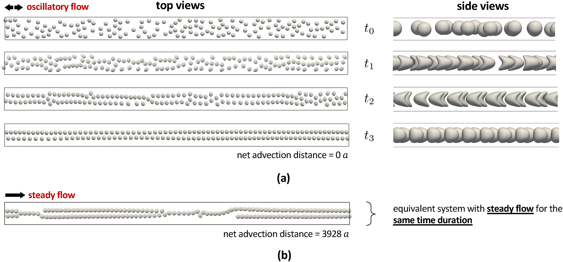Fig. 5 (a) Snapshots at progressive instances in time for ordering in oscillatory flow with Wo = 0.194, Re_max = ±1, Ca = 0.3, ϕ = 10.66%, w/a = 5.5 and h/a = 1.5. Here, t₀ corresponds to the initial state and t₃ corresponds to the final state (t̃ = 3928) which is equivalent to 10 oscillation periods for this Wo value. (b) The final particle configuration for an equivalent system in steady flow (Wo = 0) for the same time duration, i.e. time = t₃ in panel a.

Moreover, for the suspension undergoing steady flow, the net advection distance for particles is 3928a (this is roughly 23 channel lengths in the periodic flow direction). On the other hand, for the suspension undergoing oscillatory flow, the net advection distance is zero due to the fact that the sinusoidal flow cycle is symmetric in the positive and negative directions. (Note that this is not entirely true, as there are relative particle displacements associated with the time-dependent ordering process, i.e. transitioning from the initial disordered state to the final ordered state). Nevertheless, with oscillatory flows, improved ordering is found to occur and it can be facilitated without exceedingly long channels. For the oscillatory flow case, the preferred lateral spacing between trains is ∼2.8a. The ESI† contains two simulation movies of ordering in both steady and oscillatory flow conditions.

Fig. 6 displays the dependency of on Wo for five different particle deformabilities. Each data point corresponds to an individual simulation (i.e., each simulation implemented a single value of Wo). Throughout a simulation, is calculated at periodic instances in time, and the values shown in Fig. 6 are time-averaged over the last 5 × 10⁵ time steps (or the last quarter of the simulation). This was done to allow enough time for the ordering process to occur, as the initial state is a random distribution. The error bars correspond to the standard deviation in that same span. Steady flow is represented by Wo = 0, corresponding to an infinite oscillation period T. The datasets in Fig. 6 reveal that increases to one within a particular range of Wo that seems to depend slightly on Ca. Note that for the stiffest particles (Ca = 0.01 shown in Fig. 6e), there is very little improvement in particle ordering in oscillatory flows (at least for these conditions), albeit the particle ordering in steady flow is also minimal as shown in Fig. 4e. The insets in Fig. 6 provide better detail for Wo < 0.2. Overall, the flattened peaks shown in Fig. 6a–d indicate that there is an optimal range of Wo for hydrodynamic ordering.

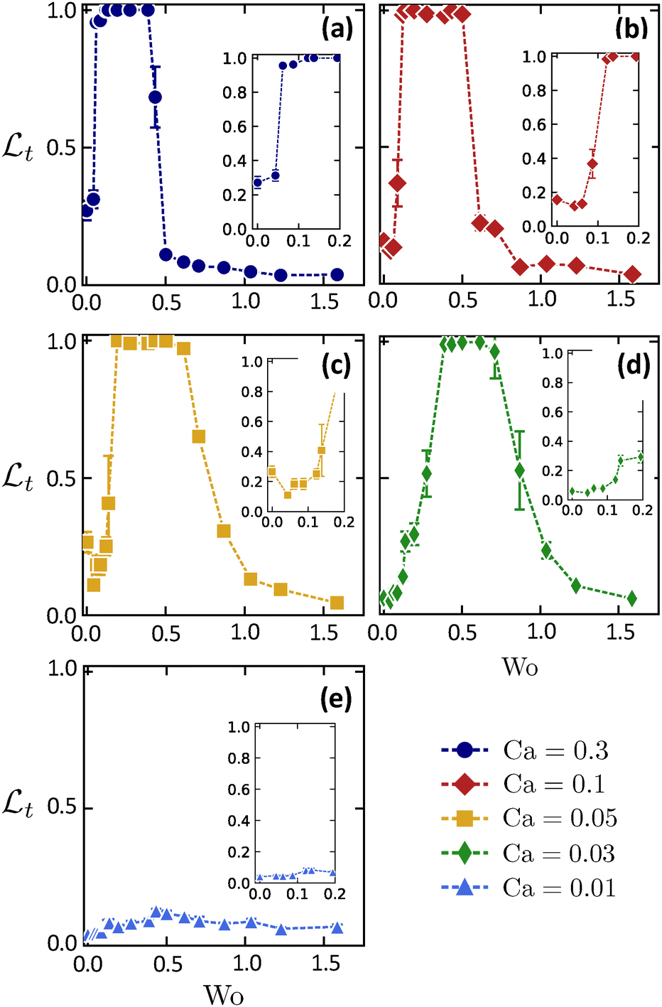Fig. 6 Order parameter versus Womersley number Wo for each of the Ca values. For each plot, the volume fraction is ϕ = 10.66%, and the channel dimensions are w/a = 5.5 and h/a = 1.5. Insets show data values for Wo < 0.2 with the same axes labels. Steady flow corresponds to Wo = 0. The results suggest an optimal range of Wo for hydrodynamic ordering for each Ca value (with the exception of Ca = 0.01 shown in panel e).

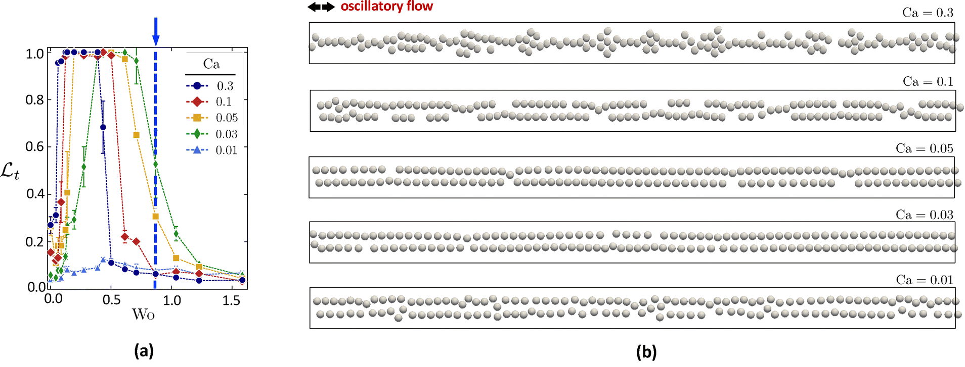
Fig. 7a displays each of the separate datasets shown in Fig. 6 on a single plot. This illustrates that the flattened peaks of shift to higher ranges of Wo with decreasing Ca. Physically, this means that stiffer particles require a higher range of Wo (i.e., a higher frequency in the oscillatory flow) to facilitate maximal ordering. Conversely, softer particles require a lower range of Wo (i.e., a lower frequency in the oscillatory flow) to facilitate maximal ordering. This can be seen in the box plot shown in Fig. 7b, displaying the optimal range of Wo (designated as Wo*) for each of the Ca values (with the exception of Ca = 0.01 corresponding to the stiffest particles, which did not achieve for any oscillatory flow condition). Finally, for each deformability value, when the Wo value exceeds 1 (and especially when the Wo value exceeds 1.5), very little hydrodynamic ordering is observed as indicated by the values being less than 0.1. Hence, it appears hydrodynamic ordering is improved with oscillatory flow only when Wo < 1 (however, this may change when Re_max is increased, something that was not done in this study).

Fig. 7 (a) Each data set shown in Fig. 6 plotted together to show that the optimal range of Wo shifts to smaller values of Wo as particle deformability increases from Ca = 0.03 to Ca = 0.3. (b) Box plot showing the optimal range of Wo (designated as Wo*) for Ca = [0.03, 0.05, 0.1, 0.3]. Note that Ca = 0.01 is not included in panel b due to a lack of ordering in this system.

To show how the particle arrangements vary with increasing Wo, Fig. 8 provides snapshots from six separate simulations for Ca = 0.1. For steady flow (Wo = 0), an extensive degree of hydrodynamic ordering occurs. In fact, nearly every particle belongs to a train (the Φ_t value is very close to 1 as shown in Fig. 10 below). However, as discussed above, for steady flow the collective ordering results in both single-file and double-file train structures, hence the value is rather low ( meaning that the average train length is only about 20% of the channel length). When Wo is increased to 0.19 as well as to 0.43, the particles assemble into two perfect double-file trains (see the second and third rows of Fig. 8b), with both simulations resulting in .

Fig. 8 Hydrodynamic ordering for Ca = 0.1 with increasing Wo. (a) The Ca = 0.1 data set (also shown in Fig. 6b) with six arrows indicating the conditions associated with the simulation snapshots shown in (b), which are taken at the end of the simulations. For Wo = 0.0 (steady flow), the particles assemble into alternating single-file and double-file trains. For Wo = 0.19 and 0.43, perfectly ordered double-file trains develop associated with . Further increasing Wo results in decreased ordering.

However, when the oscillatory frequency is further increased, we see a diminishing level of ordering as can be seen for the simulations of Wo = 0.71, 1.04, and 1.59 (the fourth, fifth, and sixth rows of Fig. 8b). For these higher levels of oscillatory frequency, it appears that there is altogether a declining amount of hydrodynamic ordering. As seen for Wo = 1.59, the particle configuration appears to be essentially random, indicating that very little to no hydrodynamic ordering has occurred throughout the simulation (even though for Wo = 1.59, the suspension has undergone 666 oscillation cycles). This can be rationalized by the fact that increasing the oscillatory frequency results in decreasing particle advection distances within a single half-cycle of the sinusoidal flow profile. As discussed by Janssen et al.,¹² the hydrodynamic ordering process is driven by quadrupolar flow disturbance fields generated by the flow-induced particle deformation. Particle–particle interactions can extend out to ∼10a.²⁰ However, if the oscillation frequency is too high, it is likely that these long-range flow fields do not have sufficient time to develop. Furthermore, with increasing oscillatory frequency the advection distance traveled by each particle decreases. These two factors will drastically reduce the overall hydrodynamic ordering throughout time.

Fig. 9 shows simulation snapshots for each particle deformability at a single oscillatory frequency, Wo = 0.87. At this particular Wo number, none of the Ca values lead to perfect ordering with , and interestingly it is the intermediate deformabilities (Ca = 0.03 and Ca = 0.05) that exhibit the highest degree of order. The softest particles (Ca = 0.3) and hardest particles (Ca = 0.01) exhibit the lowest degree of ordering. This particular Wo number is above each of the optimal ranges denoted by Wo* (see Fig. 7b). However, the optimal range for Ca = 0.03 (Wo* = 0.4–0.7) is closest to Wo = 0.87, and hence the ordering is best for this deformability.

Fig. 9 Hydrodynamic ordering for Wo = 0.87 with varying Ca. (a) The full data set (also shown in Fig. 7a) with an arrow and dashed line indicating the conditions associated with the simulation snapshots shown in (b). At this value of Wo, the ordering is best for Ca = 0.03 and 0.05. The ordering diminishes for higher deformability (Ca = 0.1 and 0.3) and also lower deformability (Ca = 0.01).

Fig. 10 displays the order parameter Φ_t (representing the fraction of particles belonging to a train) versus Wo for each particle deformability. Interestingly, increasing Wo leads to deformability-dependent trends. For the softest particles (Ca = 0.3), Φ_t is at or very close to one for Wo < 0.5. For Wo > 0.5, there is a marked decrease in Φ_t with increasing Wo. For Wo = 1.58 (the highest oscillatory frequency considered here), less than 20% of particles belong to a train, despite the fact that these are the softest particles which are very prone to ordering. On the other hand, for the stiffest particles (Ca = 0.01) Φ_t increases with Wo up to about Wo = 0.5, and then levels off at around Φ_t = 0.8. However, even though around 80% of particles belong to trains for these conditions, the is very low hence these train are quite short relative to the channel length.

Fig. 10 Order parameter Φ_t, representing the fraction of particles belonging to a train, versus Wo for each Ca value. For steady flow conditions (Wo = 0), increasing Ca results in increased Φ_t. However, increasing Wo leads to deformability-dependent trends. For the softest particles (Ca = 0.3), there is a marked decrease in Φ_t for Wo > 0.5. On the other hand, for the stiffest particles (Ca = 0.01), there is a marked increase in Φ_t with increasing Wo.

3.3. Wider channels

The above results demonstrate that oscillatory flow can effectively order a suspension of soft particles into two double-file trains in rectangular channels with a width of w/a = 5.5, in a superior manner relative to steady flow. The question arises: does oscillatory flow improve ordering in wider channels? Fig. 11a provides simulation snapshots of oscillatory ordering in rectangular channels with width w/a = 7.33 (the channel height is the same, h/a = 1.5). The volume fraction is ϕ = 12%, the particle deformability is Ca = 0.3, and the Wolmersley number is Wo = 0.194. The top image in Fig. 11a shows the initial state of randomly dispersed particles, and the third image in Fig. 11a shows the final particle configurations at the end of the simulation (recall that for these wider channels, the total number of LBM steps is 3 × 10⁶ corresponding to t̃ = 5600). As can be seen, under these oscillatory flow conditions the particles are ordered into triple-file trains with perfect order. The lateral spacing between trains is ∼3.1a (very similar to the double-file trains in Section 3.2 whereby the lateral spacing was ∼2.8a). In Fig. 11b, an equivalent system that has undergone steady flow (Wo = 0) is shown to provide a comparison. In the steady flow case, the particle arrangements consist of both double-file and triple-file trains.

Fig. 11 (a) Progressive snapshots of hydrodynamic ordering in the wider channel (w/a = 7.33 and h/a = 1.5) with oscillatory flow leading to triple-file trains. The conditions are Wo = 0.194, Ca = 0.3, and ϕ = 12.00% (number of particles = 210). The top image corresponds to the initial state. (b) The final particle configuration for an equivalent system in steady flow (Wo = 0).

For these wider channels, the versus Wo data are shown for each particle deformability in Fig. 12. These plots are similar to those given in Fig. 6. Again, we see an optimal range of Wo for particle ordering for each deformability (except Ca = 0.01). Here, corresponds to perfect triple-file trains as shown in Fig. 11a. Compared with the narrower channels (w/a = 5.5), the widths of the optimal Wo ranges are slightly less for these wider channels. This can be attributed to the fact that the confinement in the y-direction is less for these wider channels as well as the fact that it is harder to eliminate defects in larger crystalline systems. Furthermore, each of these datasets are plotting together in Fig. 13 to illustrate that again the optimal Wo values depend on Ca. Fig. 13b shows box plots of Wo* versus Ca, showing that Wo* decreases with increasing particle deformability (similar to the observations for the narrower channels shown in Fig. 7).

Fig. 12 Similar to Fig. 6, however for the wider channels (w/a = 7.33 and h/a = 1.5) and ϕ = 12.00%. Here, corresponds to perfect triple-file trains as shown in Fig. 11a.

Fig. 13 Similar to Fig. 7, however for the wider channels (w/a = 7.33 and h/a = 1.5) and ϕ = 12.00%. Here, corresponds to perfect triple-file trains as shown in Fig. 11a.

3.4. Varying particle volume fraction

Due to the lateral confinement of the rectangular channels, it is intuitive that only a certain range of particle volume fractions will facilitate the formation of perfect side-by-side train configurations (resulting in Φ_t = 1 and ). This was demonstrated earlier in Fig. 3, which showed the assembled train structures for increasing ϕ with steady flow. To quantify the dependency of particle volume fraction on ordering, Fig. 14 plots versus ϕ for a broader range of volume fractions between 3% and 14%. Two datasets are displayed: one for steady flow (Wo = 0) and one for oscillatory flow (Wo = 0.39). For both datasets, the particle deformability is Ca = 0.1 and the channel dimensions are w/a = 5.5 and h/a = 1.5.

Fig. 14 Order parameter versus volume fraction ϕ for oscillatory flow (Wo = 0.39) and steady flow (Wo = 0). For both datasets, the particle deformability is Ca = 0.1, and the channel dimensions are w/a = 5.5 and h/a = 1.5. At lower particle concentrations (ϕ = 5–6.1%), both oscillatory and steady flows result in single-file trains (similar to that shown in Fig. 3b). However, at higher particle concentrations (ϕ = 10–12.5%), only oscillatory flows result in perfect double-file trains.

Fig. 14 shows that at lower particle concentrations (ϕ = 5.0–6.1%), both oscillatory and steady flows result in single-file trains, similar to that shown in Fig. 3b. This is perhaps to be expected, given the fact that deformable particles tend to migrate to the channel centerline,³⁷ thus facilitating the formation of a single-file train along this centerline at volume fractions that allow the particle spacing to be at, or close to, the equilibrium spacing. When ϕ is increased to the range of 6.1–9.5%, the values drop to around 0.1 for both oscillatory and steady flow. This volume fraction range is intermediate in the sense that it is too high to form a single-file train and too low to form double-file trains, hence the resulting structure is the combination of single and double-file trains, similar to those shown in Fig. 3c–e. However, for the volume fraction range of ϕ = 10–12.2%, we see that only oscillatory flows result in perfect double-file trains. These results suggest that oscillatory flows facilitate improved hydrodynamic ordering for the assembly of multiple side-by-side trains within a rectangular channel, and that oscillatory flows can accomplish this for a range of ϕ rather than for only one specific value of ϕ.

3.5. Polydisperse suspensions

Lastly, attention is turned to how polydispersity in particle radius affects hydrodynamic ordering in both steady and oscillatory flows. Here, a Gaussian distribution in particle radius is assigned to the suspension, and the polydispersity is quantified by the standard deviation in particle radius divided by the channel half height (in other words, the standard deviation of the ratio a/h). This standard deviation is represented as σ_a/h. Fig. 15a shows a histogram of probability P (in percent) versus a/h for σ_a/h = 0.044. For all simulations in this section, the mean a/h value is 0.667 (corresponding to h/a = 1.5 as was the case for all of the above results) and increasingly wider distributions in particle radius, or larger values of σ_a/h, are considered.

Fig. 15 (a) Histogram of the distribution of reduced particle radius (a/h) in a polydisperse suspension with a standard deviation of σ_a/h = 0.044. (b) Order parameter versus σ_a/h for oscillatory flow (Wo = 0.27) and steady flow (Wo = 0). For this data, Ca = 0.3, ϕ = 10.66%, and the channel dimensions are w/a = 5.5 and h/a = 1.5. Note: σ_a/h = 0 corresponds to a monodisperse suspension.

Fig. 15b shows versus σ_a/h for both oscillatory flow (Wo = 0.27) and steady flow (Wo = 0). Note that σ_a/h = 0 corresponds to a completely uniform, monodisperse suspension. For both of these datasets, the particle deformability is Ca = 0.3, the particle volume fraction is ϕ = 10.66%, and the channel dimensions are w/a = 5.5 and h/a = 1.5 (note that the a used here now corresponds to mean particle radius). For monodisperse suspensions with σ_a/h = 0, the order parameter for Wo = 0.27 and for Wo = 0. This is consistent with the above results demonstrating that oscillatory flow orders particles into perfect double-file trains while steady flow does not. Increasing polydispersity leads to a decrease in for both oscillatory and steady flow conditions. However, for oscillatory flow, the drop-off in does not occur until σ_a/h > 0.02.

Images of the final particle configurations in polydisperse suspensions are provided in Fig. 16. For the case of oscillatory flow (Fig. 16a), perfect double-file trains have developed for σ_a/h = 0.0056. Increasing σ_a/h to 0.0333 leads to some localized defects and variability in particle spacing within the train structures. Further increasing σ_a/h to 0.0556 results in more defects, however the overall semblance of the double-file train structures remains. On the other hand, for the case of steady flow (Fig. 16b), increasing the polydispersity of the suspension significantly reduces the assembly of train structures, and therefore the overall order within the system. This can be seen particularly for the case of σ_a/h = 0.0556.

Fig. 16 Simulation snapshots of final particle configurations in polydisperse suspensions for (a) oscillatory flow (Wo = 0.27) and (b) steady flow (Wo = 0). For each case, three different values of σ_a/h are shown, corresponding to increasing degrees of polydispersity. Oscillatory flow is significantly better at ordering suspensions with higher polydispersity. The lightly shaded boxes are shown in close-up views in Fig. 17.

In Fig. 16, there are two lightly-shaded boxes - one for the oscillatory flow simulation and one for the steady flow simulation (both for the case of σ_a/h = 0.0333). Close-up views of these regions are given in Fig. 17 including both top-down and side views, providing better depictions of the variation in particle size. Overall, these results suggest that oscillatory flow facilitates more robust particle ordering even with increasing polydispersity in the particle radius.

Fig. 17 Close-up views of the shaded boxes in Fig. 16, including top-down and side views. These images better depict the variation in particle size. (a) Close-up image of particle configurations for Wo = 0.27 and σ_a/h = 0.0333. (b) Close-up image of particle configurations for Wo = 0.00 and σ_a/h = 0.0333.

4. Conclusions

Arranging particles into a single-file configuration is advantageous, and in some cases necessary, for many technological applications including cytometry, bio-assay, and bottom-up manufacturing. Here, three-dimensional IBM/LBM simulations were performed to investigate how hydrodynamic ordering of soft suspensions is altered by oscillatory flow compared to steady flow in highly confined rectangular channels. The primary conclusions of this work are:

1. Hydrodynamic ordering is improved with oscillatory flow relative to steady flow, with an optimal range of Wo number that depends on the particle deformability. For softer particles (Ca = 0.3), 0.1 < Wo < 0.3 is optimal for ordering. This range increases slightly with increasing particle stiffness. For stiffer particles (Ca = 0.03), 0.4 < Wo < 0.7 is optimal for ordering. See Fig. 7 and 13. For all deformabilities, hydrodynamic ordering diminishes significantly for Wo > 1.

2. Oscillatory flow better facilitates the ordering of multiple side-by-side trains, including double-file and triple-file trains (depending on the cross-sectional channel dimensions and particle volume fraction). In this work, multiple side-by-side trains with were not observed to form in steady flow conditions.

3. Oscillatory flow is more robust for ordering suspensions with polydispersity in particle radius. As polydispersity increases, the ordering of double-file trains was better preserved with oscillatory flow relative to steady flow (see Fig. 15–17).

Although this study explored several parameters and parameter ranges, there are still outstanding questions on this topic that require further investigation. In particular, here the amplitude of the flow rate was not varied (it was fixed at Re_max = ±1). It will be interesting to determine if increasing this amplitude will broaden or shift the optimal Wo ranges discussed above. In addition, questions regarding how many side-by-side trains can be assembled with increasing channel width will be important to determine.

Data availability

The code for the IBM/LBM simulations was written by the author and is titled “FlowCUDA.” It can be found at https://github.com/paulmillett/FlowCUDA.

Conflicts of interest

There are no conflicts to declare.

Acknowledgements

PCM gratefully acknowledges financial support from the 21st Century Endowed Professorship provided by the University of Arkansas. This research is also supported by the Arkansas High Performance Computing Center which is funded through multiple National Science Foundation grants and the Arkansas Economic Development Commission.

Notes and references

1. J.-P. Matas, V. Glezer, É. Guazzelli and J. F. Morris, Phys. Fluids, 2004, 16, 4192–4195.
2. D. Di Carlo, D. Irimia, R. G. Tompkins and M. Toner, Proc. Natl. Acad. Sci. U. S. A., 2007, 104, 18892–18897.
3. J. F. Edd, D. D. Carlo, K. J. Humphry, S. Köster, D. Irimia, D. A. Weitz and M. Toner, Lab Chip, 2008, 8, 1262–1264.
4. W. Lee, H. Amini, H. A. Stone and D. Di Carlo, Proc. Natl. Acad. Sci. U. S. A., 2010, 107, 22413–22418.
5. K. J. Humphry, P. M. Kulkarni, D. A. Weitz, J. F. Morris and H. A. Stone, Phys. Fluids, 2010, 22, 081703.
6. C. Schaaf and H. Stark, Eur. Phys. J. E: Soft Matter Biol. Phys., 2020, 43, 50.
7. J. Liu, H. Liu and Z. Pan, Phys. Fluids, 2021, 33, 073301.
8. B. Chun and A. J. C. Ladd, Phys. Fluids, 2006, 18, 031704.
9. S. Kahkeshani, H. Haddadi and D. Di Carlo, J. Fluid Mech., 2016, 786, R3.
10. J. L. McWhirter, H. Noguchi and G. Gompper, Proc. Natl. Acad. Sci. U. S. A., 2009, 106, 6039–6043.
11. J. L. McWhirter, H. Noguchi and G. Gompper, New J. Phys., 2012, 14, 085026.
12. P. J. A. Janssen, M. D. Baron, P. D. Anderson, J. Blawzdziewicz, M. Loewenberg and E. Wajnryb, Soft Matter, 2012, 8, 7495–7506.
13. G. Tomaiuolo, L. Lanotte, G. Ghigliotti, C. Misbah and S. Guido, Phys. Fluids, 2012, 24, 051903.
14. S. H. Bryngelson and J. B. Freund, Phys. Rev. Fluids, 2016, 1, 033201.
15. Z. Shen, T. M. Fischer, A. Farutin, P. M. Vlahovska, J. Harting and C. Misbah, Phys. Rev. Lett., 2018, 120, 268102.
16. S. Singha, A. R. Malipeddi, M. Zurita-Gotor, K. Sarkar, K. Shen, M. Loewenberg, K. B. Migler and J. Blawzdziewicz, Soft Matter, 2019, 15, 4873–4889.
17. S. Ishida, R. Matsumoto, D. Matsunaga and Y. Imai, Phys. Rev. Fluids, 2022, 7, 063601.
18. M. Abkarian, M. Faivre, R. Horton, K. Smistrup, C. A. Best-Popescu and H. A. Stone, Biomed. Mater., 2008, 3, 034011.
19. C. Iss, D. Midou, A. Moreau, D. Held, A. Charrier, S. Mendez, A. Viallat and E. Helfer, Soft Matter, 2019, 15, 2971–2980.
20. P. C. Millett, J. Fluid Mech., 2024, 979, A29.
21. B. Dincau, E. Dressaire and A. Sauret, Small, 2020, 16, 1904032.
22. S. M. McFaul, B. K. Lin and H. Ma, Lab Chip, 2012, 12, 2369–2376.
23. K. Ward and Z. H. Fan, J. Micromech. Microeng., 2015, 25, 094001.
24. M. Abolhasani and K. F. Jensen, Lab Chip, 2016, 16, 2775–2784.
25. P. Zhu and L. Wang, Lab Chip, 2016, 17, 34–75.
26. Y. Yoon, S. Kim, J. Lee, J. Choi, R.-K. Kim, S.-J. Lee, O. Sul and S.-B. Lee, Sci. Rep., 2016, 6, 26531.
27. D. Cheng, Y. Yu, C. Han, M. Cao, G. Yang, J. Liu, X. Chen and Z. Peng, Biomicrofluidics, 2018, 12, 034105.
28. J. Lee, S. E. Mena and M. A. Burns, Sci. Rep., 2019, 9, 1278.
29. J. E. Butler, P. D. Majors and R. T. Bonnecaze, Phys. Fluids, 1999, 11, 2865–2877.
30. J. F. Morris, Phys. Fluids, 2001, 13, 2457–2462.
31. J. Cui, H. Wang, Z. Wang, Z. Zhu and Y. Jin, Int. J. Mech. Sci., 2024, 278, 109471.
32. J. Maestre, J. Pallares, I. Cuesta and M. A. Scott, J. Mech. Behav. Biomed. Mater., 2019, 90, 441–450.
33. N. Takeishi, K. Ishimoto, N. Yokoyama and M. E. Rosti, J. Fluid Mech., 2025, 1008, A46.
34. P. C. Millett, Soft Matter, 2023, 19, 1759–1771.
35. R. Skalak, A. Tozeren, R. P. Zarda and S. Chien, Biophys. J., 1973, 13, 245–264.
36. A. J. C. Ladd, J. Fluid Mech., 1994, 271, 285–309.
37. C. Schaaf and H. Stark, Soft Matter, 2017, 13, 3544–3555.

---

Footnote

† Electronic supplementary information (ESI) available. See DOI: https://doi.org/10.1039/d5sm00422e

---