DOI:
10.1039/D4SM01433B
(Paper)
Soft Matter, 2025,
21, 5323-5336
A rate dependent interface model for stick-slip fracture in adhesives and polymer glasses†
Received
2nd December 2024
, Accepted 14th May 2025
First published on 19th May 2025
Abstract
In stick-slip fracture, a crack stays still or only propagates a small amount until it reaches a critical energy release rate. Then, it suddenly grows rapidly, causing the energy release rate to drop and the crack to stop again. This behavior is common in many polymers, including glassy polymers and soft materials like adhesives. However, the theoretical understanding of this phenomenon is fragmented and incomplete. Here we propose a unified theory based on a rate-dependent cohesive model to explain these phenomena. Using this model, we demonstrate that an elastic backing layer in a zero-degree peel test can experience different types of stick-slip instability depending on the peeling rate. At slow peeling rates, the crack grows slowly until it reaches a maximum velocity, corresponding to a fixed maximum force, after which the growth becomes unstable. However, above a certain critical peeling rate, there is no slow crack growth: the crack enters the stick-slip regime once the critical energy release rate is reached for a reduced value of the applied force. Although our mathematical modeling is developed in a specific geometry that makes the computations easier, this behavior can be argued to be a more general feature of most materials and geometries presenting stick-slip fracture.
Introduction
Stick-slip fracture in polymer systems often refers to the situation where a crack stays still or only propagates a very small amount until the specimen reaches a critical load. Then, the crack suddenly grows rapidly, causing the specimen to unload and the crack to stop again. When specimens are loaded with a constant loading rate, this process can repeat itself and is commonly observed in peeling of adhesive tapes1 and in fracture tests of thermoplastics (e.g., PMMA)2 and thermosets (e.g., epoxy).3
Stick-slip fracture is often modeled using a kinetic relationship between a velocity dependent fracture toughness (Γ) and the steady-state crack growth rate (v), as shown in Fig. 1. During crack growth, the velocity dependent fracture toughness equals the energy release rate G, which depends solely on specimen geometry and external loading. It is typically assumed that this relationship applies even during non-steady-state crack growth, motivating the development of differential equations to predict the dynamics and duration of stick-slip cycles.4–6
 |
| | Fig. 1 Schematic of velocity dependent toughness Γ versus crack velocity v for stick-slip dynamics. vΓmax and vΓmin are the crack velocities corresponding to Γmax and Γmin respectively. The dashed black line indicates the unstable branch where crack growth cannot be sustained. As a result, when the crack velocity reaches vΓmax, it jumps to the slip branch (solid black line on the right), where crack growth is much faster than the loading rate. This jump from stick branch (solid black line on the left) to the slip branch is indicated by the upper red arrow. Since loading is displacement controlled, the crack gradually slows down and reaches vΓmin, after which it re-enters the stick branch, as indicated by the lower red horizontal arrow. | |
In the peeling of adhesive tapes, the fracture toughness Γ versus crack velocity v plot can be divided into three branches as shown in Fig. 1. On two of these branches (black solid lines), crack growth is stable, and the energy release rate required for crack growth increases with crack velocity. One branch corresponds to slow crack velocity (v < 10−2 m s−1 in general), while the other corresponds to fast or dynamic crack velocity (v > 1 m s−1). These two branches are connected by an unstable branch (dashed black line) where stick-slip occurs. Although the existence of a negative slope branch of the energy release rate is supposed to link the two stable branches, this cannot be directly measured in experiments since the steady-state solution would be unstable. Some papers report that, in this region, the maximum strain energy release rate (or the maximum force) experienced during stick-slip cycles-indicated by the red arrows in Fig. 1, decreases with increasing pulling velocity applied to the adhesive tape.4
In PMMA, the slow quasi-static crack growth regime typically spans several decades of crack velocities (from 10−9 m s−1 to 10−1 m s−1),7 while the range of dynamic crack growth is comparatively small (102 m s−1–103 m s−1). The maximum strain energy release rate experienced during the stick-slip regime does not depend on the sample loading velocity for PMMA.2 In epoxy polymers, the crack often remains static until it reaches a critical energy release rate. After this point, the crack grows intermittently in a stick-slip manner without experiencing a slow crack growth phase. However, Nziakou et al.8 have demonstrated that this slow branch is difficult to observe because the crack velocity on this branch is limited to less than 10−9 m s−1. Moreover, the critical energy release rate to initiate the dynamic crack propagation in the stick phase (or the maximum force during the stick-slip cycles), is found to decrease with the loading velocity of the sample.3
Fig. 1 illustrates the classical cyclic picture of stick-slip dynamics. Beginning with a slow loading rate (e.g., peeling velocity in a peel test), the crack velocity grows slowly until it reaches a critical velocity, vΓmax. At vΓmax, crack growth becomes unstable, and the propagation enters the dynamic crack propagation in the fast “slip” branch. During slip, the system unloads because the crack growth rate is much faster than the loading rate, causing the crack to slow down along the slip branch. When a second critical velocity vΓmin is reached, the crack velocity suddenly jumps back to the slow “stick” branch, and everything starts again leading to periodic stick-slip cycles as indicated by the red arrows in Fig. 1.
Although stick-slip occurs in both soft materials like adhesives and hard materials like polymer glasses, their fracture mechanics differ significantly. In polymer glasses, the fracture process zone (e.g., the size of the plastic zone) is much smaller than typical specimen dimensions, allowing the application of linear elastic fracture mechanics (LEFM). This means that there is a region near the crack tip where the singular fields generated by a sharp crack dominate. In contrast, the fracture of adhesives is dominated by large strain mechanics and non-linear rheology, as evident by cavitation and fibrillation of the adhesive layer during peeling.9 Specifically, the stress/strain singularity associated with a sharp crack is eliminated since the size of the fibrillated region is comparable to or larger than the thickness of the adhesive layer.
Until recently, no comprehensive theory has addressed all these features, especially as they occur in different material systems such as thermosets, thermoplastics, and adhesives. In a recent work, Nziakou et al.8 proposed a scaling theory to link these features into a unified model. Here, we propose a simple analytic model that captures the essence of their approach. Unlike scaling theory, our approach is quantitative, providing precise mathematical formulations and detailed analysis. While scaling theory often relies on order of magnitude estimates, our method employs a rate-dependent cohesive model to quantify the fracture process. This approach provides specific predictions and insights about the behavior of various material systems under different loading conditions.
In this paper, we use the zero-degree peel test (Fig. 2) to define the loading geometry of an adhesive tape, although most experiments typically employ the 90-degree peel configuration. For peel angles greater than or equal to 30 degrees, the toughening mechanism is known to involve the stretching of fibrils formed by cavitation in the highly constrained region ahead of the peel front or crack tip. The rate-dependent cohesive zone model described in the next section is motivated by the extension and rupture of these fibrils during peeling. However, it should be noted that cavitation is not observed at low peel angles, where shear dominates and failure is primarily due to frictional and adhesive slippage. We adopt the zero-degree geometry in this work to simplify the mechanics of load transfer between the adhesive and the extensible backing. Since our focus is on illustrating fundamental concepts rather than comparing theory with experimental data, the zero-degree peel test is chosen for its analytical simplicity and the availability of exact closed-form solutions.
 |
| | Fig. 2 Geometry of zero-degree peel, the adhesive in this case is an infinitely thin layer between the elastic layer (in blue) and the rigid substrate (in dark grey). The cohesive zone between the elastic layer and the rigid substrate is highlighted as a thick line in yellow even though it has zero thickness, and the dark green line indicates that the substrate and the elastic layer are perfectly bonded with no slip. The region x > −c is not in contact and is not part of the cohesive zone. | |
A rate dependent cohesive model
The key aspect of our analysis is the use of a rate-dependent cohesive model to describe the fracture process. For a comprehensive background and review of the cohesive zone model, please refer to ref. 10–13. To motivate our model, we observe that during the steady-state peeling of adhesive tapes, each fibril in the cavitated adhesive layer directly ahead of the crack tip experiences the same loading history: it stretches upon formation and eventually breaks at the peel front. Both the average stress and the maximum stretch ratio of a fibril, and consequently the energy dissipated during stretching, are influenced by the local strain rate. The energy dissipated during the stretching systematically increases with the strain rate, reaches a peak, and then decreases. While the average stress is generally a slowly increasing function of strain rate driven by the rheological response of the adhesive, the maximum fibril stretch can experience both increasing and decreasing dependency on the strain rate depending on the kind of adhesive.14 This complex dependency on the strain rate can be explained by the modulation of stress transfer from the dense entangled network to the sparse cross-linked network, which is strongly dependent on the specific structure of the polymer network of the adhesive. Here, we assume for simplicity that the cohesive stress is constant while the maximum extension of a fibril increases with the strain rate, reaches a peak, and then decreases. This captures the most general behavior while providing the simplest form of analytical solutions for the stress distribution and crack propagation problem. The deformation of fibrils is represented by the interfacial displacement jump δ between the peel arm (or backing layer) and the rigid substrate (see Fig. 2).
Our model in a zero-degree peel test specifies a relation between the shear displacement jump or slip δ across the backing/substrate interface (indicated by yellow line in Fig. 2) and the interfacial shear stress τ by:
| |  | (1) |
where

is the time rate of shear displacement or slip rate.
Eqn (1) applies to an interface continuum point, so
δ and

can vary spatially and temporally. Motivated by the mechanics of fibril stretching described above, the shear stress response function
Φ has the following characteristics: the work to debond the interface first increases with the slip rate, reaches a maximum at some rate, then decreases to some constant value afterward.
We assume the simplest model: a rate dependent Dugdale–Barenblatt (DB) model, in which the interfacial shear stress maintains a constant value τ0 when the slip is less than a critical threshold denoted by δc. For δ > δc, the interface fails and offers no resistance to shear, i.e.,
| |  | (2a,2b) |
where

,
δ0 are material constants.

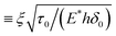
is a characteristic slip rate and
δ0 is the critical slip at zero slip rate. In this model the energy required to debond a unit area of the interface, or the interfacial toughness is
Γc =
τ0δc. In the classical DB model,
δc is independent of slip rate, but here we assume
δc depends on the slip rate through the response function
ϕ(
η) where

. Note by definition,
| |  | (3) |
where
Γ0 =
τ0δ0 is the interfacial toughness at zero slip rate. In the following, we assume
ϕ(
η) increases from 1 at
η = 0 to its local maximum
ϕmax at
ηmax > 0. On this ascending branch,
η ∈ (0,
ηmax),
ϕ′(
η) = d
ϕ/d
η > 0. For
η >
ηmax,
ϕ decreases monotonically to 1. On this descending branch,
ϕ′(
η) ≤ 0. The schematic of
ϕ is shown in
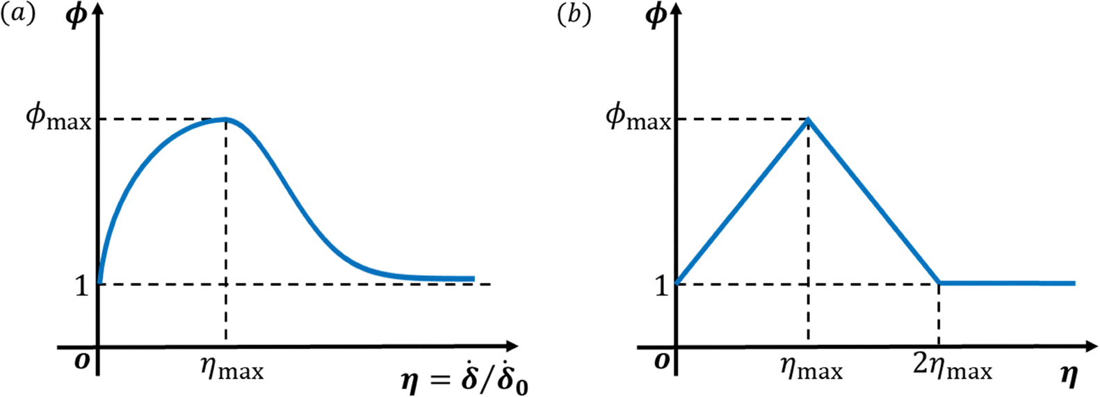
Fig. 3.
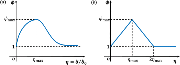 |
| | Fig. 3 Schematic of ϕ = δc/δ0 as a function of  . (a) Shows a general function of ϕ(η) which starts at ϕ(η = 0) = 1, monotonically increases to ϕmax at η = ηmax and then monotonically decreases to 1 as η → ∞. (b) Is the piecewise-linear function we use in this paper for analytical analysis in the section called fracture initiation. . (a) Shows a general function of ϕ(η) which starts at ϕ(η = 0) = 1, monotonically increases to ϕmax at η = ηmax and then monotonically decreases to 1 as η → ∞. (b) Is the piecewise-linear function we use in this paper for analytical analysis in the section called fracture initiation. | |
Mechanics of zero-degree peel test
Both the adhesive layer and the elastic backing layer are assumed to be very thin in comparison with their lateral dimensions. In the peel test, out-of-plane deformation is negligible since the width of the tape is much larger than its thickness, resulting in a plane strain condition with zero out-of-plane strain. This allows us to use a one dimensional shear-lag model to model the load transfer mechanics.15 In this model, the elastic layer is in a state of uniaxial tension σ. The equilibrium equation governing the change in σ inside the cohesive zone is:| |  | (4) |
where u and E* are the displacement and plane strain modulus of the elastic backing layer respectively, l is the length of the cohesive zone, c is the crack length or the length of the peel arm and h is thickness of the backing layer. Note inside the cohesive zone,| | | u(x,t) = δ(x,t), x ∈ (−l −c, −c) | (5) |
Ahead of the cohesive zone tip in x < −l −c, u = δ = 0. Combining (4)–(5) and (2a), (4) becomes
| |  | (6) |
In the elastic layer behind the crack tip, force balance implies that the force acting on the peel arm F is
| |  | (7a) |
The elastic backing is loaded by displacement control, and we denote
to be the applied displacement at the loading point. The presence of cohesive zone allows us to impose continuity of displacement at the crack tip,
i.e.,
| | | δtip ≡ δ(x = −c,t) = u(x = −c,t) | (7c) |
Normalization
We normalize all lengths by a load transfer length  and displacements by δ0
| |  | (8) |
Using this normalization, eqn (6) simplifies to
| |  | (9) |
where
C,
L, and
Δ are the normalized crack length, normalized length of the cohesive zone and normalized slip respectively. Assuming loading starts at
t = 0, the initial condition (IC) is:
The boundary conditions (BCs) are:
| |  | (11a-c) |
where
Δtip denotes the normalized slip at the crack tip. The solution of
(9) that satisfies the BCs
(11b, c) is
| |  | (12) |
The length of the cohesive zone
L is determined by
(11a),
i.e.,
| |  | (13) |
According to (12), the maximum slip occurs at the crack tip X = −C and is Δtip. The normalized length of the slip zone is  .
.
Relation between applied displacement uA(t) and normalized slip at crack tip Δtip(t)
To relate the applied displacement uA(t) to δ(x = −c,t), we use continuity. The presence of the cohesive zone allows for the continuity of strain on the peel arm at x = −c. The tensile strain is spatially constant in the peel arm and is| |  | (14) |
By continuity, (14) is also the tension strain at the crack tip, which is obtained using (12), i.e.,
| |  | (15) |
Equating (14) and (15) and using (13) and the normalization (8), the normalized applied displacement UA(t) ≡ uA(t)/δ0 and the normalized slip at the crack tip Δtip(t) are related to each other by
| |  | (16a) |
where
| |  | (16b) |
Note C is the normalized crack length, and β is directly proportional to it by the factor  . From here on, we will refer to either C or β as the normalized crack length.
In the following, we introduce a normalized time T by
| |  | (17) |
We assume a constant displacement rate,  , is applied to the peel arm at x = 0, where α is the normalized peel rate, i.e.,
| |  | (18) |
Using (18), the maximum normalized slip at the crack tip (16a) is
| |  | (19) |
Note that we have not restricted the crack length to be stationary, i.e., β can be a function of time.
Fracture criterion
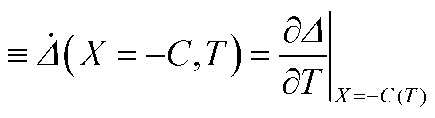
The condition of fracture is| |  | (20a) |
The normalized form of (20a) (recall δ(x = −c,t) = δ0Δtip(T)) is
| |  | (20b) |
Here we note that  in (20b) depends on both the crack motion and the loading rate. Specifically, using (12),
| |  | (20c) |
The last term in
(20c) indicates that there are two contributions to the local strain rate at the crack tip, the first one is due to crack growth, and the other is due to external loading. To distinguish

from d
Δtip(
T)/d
T, we denote

with a dot. Only in the special case of a stationary crack where d
C/d
T = 0, does
. Note for the special case of steady-state crack growth, d
Δtip(
T)/d
T = 0 and

.
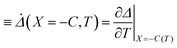
The physical interpretation of (20b) is as follows: the left-hand side (LHS) is the normalized energy release rate, while the right-hand side (RHS) represents the normalized intrinsic toughness, which depends on both the loading rate and the crack growth rate (for more details, see ESI†). These two (external loading rate and crack growth rate) compete. To see this and to unravel the features noted in the introduction, we consider two situations: crack initiation and the subsequent crack growth in a constant displacement rate test.
For crack initiation, the crack is stationary, so the normalized crack length C and  are independent of time, the local slip rate is obtained by setting dC/dT = 0 in (20c) and evaluating
  using (19), this results in
| |  | (21a) |
For the case of a growing crack, the local slip rate at the crack tip is obtained using
(20c), (13) and (19):
| |  | (21b) |
Note the effect of loading rate α and crack growth rate dβ/dT on the rate of energy flow to the crack tip is coupled since the crack growth rate and loading rate both appear in  . Also, when crack growth rate is zero, (21b) reduces to (21a).
Fracture initiation
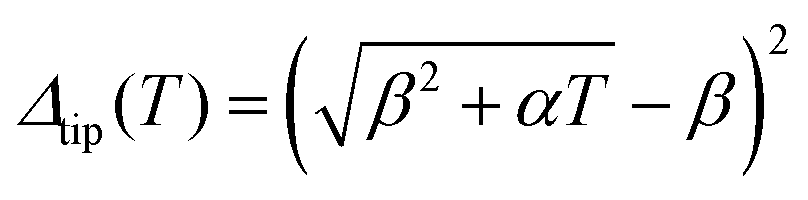
To study fracture initiation, we substitute (21a) into (20b) and use (19) to determine the normalized crack initiation time, TI, which must satisfy| |  | (22) |
The dependence of crack initiation time on crack length, loading rate, and the response function ϕ is of particular interest. Additionally, how the loading rate influences whether crack initiation occurs on the ascending or descending branch is crucial, since, as we will show in the next section, crack growth on the descending branch is unstable. Interestingly, these questions can be explored for any arbitrary continuous ϕ.
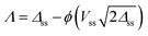
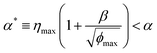
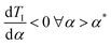
We state a key result in this paper: for any arbitrary continuous ϕ(η) that has an ascending branch followed by a descending branch (with a maximum value ϕmax at η = ηmax), there exists a critical normalized loading rate α* given by
| |  | (23) |
the crack initiation time corresponding to α* is
| |  | (24) |
At this critical rate, the normalized energy release rate
Δtip reaches its maximum value
ϕmax. In the appendix, we show that initiation always occurs on the ascending branch of
ϕ for
α <
α*. Note in particular,
ηmax <
α* by
eqn (23). For
α >
α*, initiation always occurs on the descending branch of
ϕ. The proof of these results is given in the appendix. It is interesting to note that
(23) and (24) imply that the critical loading rate increases linearly with crack length and is directly proportional to
ηmax while the critical initiation time is inversely proportional to
ηmax and is rather insensitive to the crack length.
To illustrate these results, we use the special case of a piece-wise linear shear response function ϕ (illustrated in Fig. 3(b)) where
| |  | (25a-c) |
Fig. 4 plots the LHS of (22), i.e.,  as solid lines, and the RHS of (22), i.e.,
  as dash-dot lines, both plotted against the normalized time T for different values of α. For each value of α, the RHS and LHS of (22) generate two curves. Note that the LHS of (22) is a monotonically increasing function of T with increasing slope whereas the RHS of (22) increases, reaches a maximum, and then decreases. As a result, the two curves intersect at a single point, which gives the initiation time TI. In Fig. 4, we use β = β0 = 1, ϕmax = 4, and ηmax = 1. The critical loading rate α* = 3/2 with
  is used as a reference. An interesting result shown in Fig. 4 is that the initiation time decreases with increasing α.
 |
| | Fig. 4 Illustration of theory using (25a–c). The functions in (22), i.e.,  (solid lines) and (solid lines) and  (dash-dot lines) are plotted against normalized time T for 6 different normalized loading rates α. The intersection of these curves, indicated by a circle, gives the initiation time TI. (For α = 0.375, the initiation time TI exceeds beyond the maximum plotted time of 10 and is therefore not displayed.) The curves are generated using β = β0 = 1, ϕmax = 4, and ηmax = 1. For this case, the critical loading rate is α* = 1.5. Consistent with theory, initiation occurs on the ascending/descending branch for α < α*/α > α* respectively. (dash-dot lines) are plotted against normalized time T for 6 different normalized loading rates α. The intersection of these curves, indicated by a circle, gives the initiation time TI. (For α = 0.375, the initiation time TI exceeds beyond the maximum plotted time of 10 and is therefore not displayed.) The curves are generated using β = β0 = 1, ϕmax = 4, and ηmax = 1. For this case, the critical loading rate is α* = 1.5. Consistent with theory, initiation occurs on the ascending/descending branch for α < α*/α > α* respectively. | |
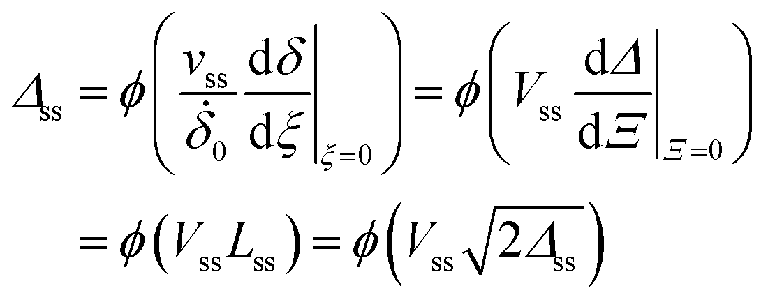
Steady-state crack growth (SSCG)
To proceed further, we take a slight detour to examine the role of the ascending and descending branch of the shear response function ϕ on the stability of crack growth. This is accomplished by considering steady-state crack growth (SSCG) – an idealization where the stress and strain fields in a cracked body translate rigidly with a coordinate system attached to the crack tip which grows at a constant velocity vss > 0. For the case of zero-degree peel test, steady-state condition requires that the fields depend only on ξ = c0 + x + vsst, where ξ is the coordinate of a frame moving with the crack tip, c0 is the crack length where steady-state is reached (set as t = 0). Mathematically, the steady-state condition (SS) is:| |  | (26) |
Note that (9) is independent of rate, so the equation governing slip distribution is the same as (9) with x → ξ. Using the same normalization, the BCs are:
| |  | (27a-c) |
Following the same line of reasoning, the slip distribution inside the cohesive zone is:
| |  | (28) |
Next, we determine the steady-state crack velocity vss using the fracture condition (20a), i.e.,
| |  | (29a) |
where
| | 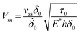 | (29b) |
is the normalized steady-state crack velocity. As noted in
(3),
ϕ has the property that
ϕ(
η = 0) = 1. Recall that
ϕ increases from
η = 0 to
η =
ηmax, reaches a maximum
ϕmax, then decreases afterwards. Since we assume that
ϕ cannot be less than 1, there is no solution for SSCG if
Δss < 1.
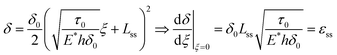
To gain a deeper understanding of the requirement for steady-state, we apply energy balance analysis. Let Fss denote the constant peel force exerted at the end of the peel arm which is subjected to a constant strain εss, they are related by
The strain in the peel arm is:
| |  | (31) |
Note because of steady-state, the slip distribution inside the cohesive zone is independent of time, hence the terms inside the bracket in the RHS of
(31) are independent of time. It is important to note that the applied displacement must increase linearly with time while peel force remains constant since material is added to the peel arm during crack growth. Using
(31), this condition is
| |  | (32) |
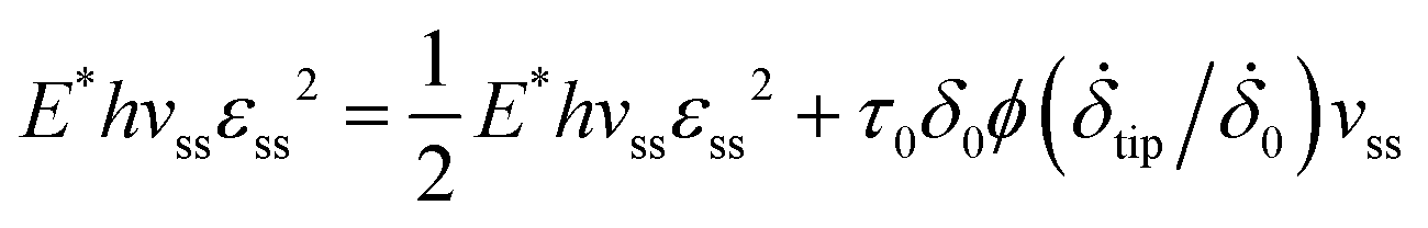
In steady-state, the rate of energy input must be constant and is given by
| |  | (33) |
where we have used
(30) and (32). Energy balance requires this energy input rate must be balanced by the rate of increase in strain energy of the peel arm and the work of decohesion,
i.e.,
| |  | (34a) |
After cancellation, (34a) is
| |  | (34b) |

in
(34b) can be obtained using steady-state condition
(26) and is
| |  | (35) |
where we have used continuity of strain at the crack tip. Indeed, according to
(28),
| |  | (36) |
Substituting (35) and (36) into the energy balance eqn (34b), we obtain
| |  | (37) |
With
(28) and (37) becomes identical to the fracture condition in
(29a).
We study stability of crack growth by imposing a small perturbation in the crack velocity and examining the change in the energy functional (see (29a))
| |  | (38) |
which represents the difference between the normalized energy release rate and the normalized intrinsic toughness. Crack growth is unstable if
| |  | (39) |
However, since
Δss is proportional to
εss2 (see
(28) and (36)) and the peel test is displacement controlled, which means that the perturbation is carried out at fixed
Δss, so the
(39) becomes:
| |  | (40) |
Note on the descending branch where

,
(40) is satisfied, so steady-state crack growth is always unstable on this branch.
A simple example is when ϕ is given by (25a–c), SSCG is stable on the ascending branch since  . Note when Δss = ϕmax, the maximum velocity for stable crack growth is reached, which is
| |  | (41) |
Non-steady-state crack growth: stick-slip
In this section we study non-steady-state crack growth. As before, we assume that the peel arm is loaded at a constant displacement rate. We first assume the loading velocity α < α* so crack initiation occurs on the ascending branch. To ensure that the slope of the shear response function at ηmax is continuous, ϕ is now taken to be quadratic, i.e.,| |  | (42) |
During crack growth, the fracture criterion is determined using (19), (20b) and (21b), i.e.,
| |  | (43a) |
Eqn (43a) is a nonlinear ordinary differential equation for β with initial condition
where
β0 is the initial normalized crack length. Recall

, so it is a different normalization of the crack length.
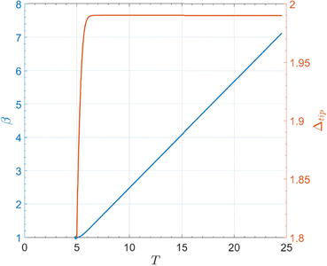
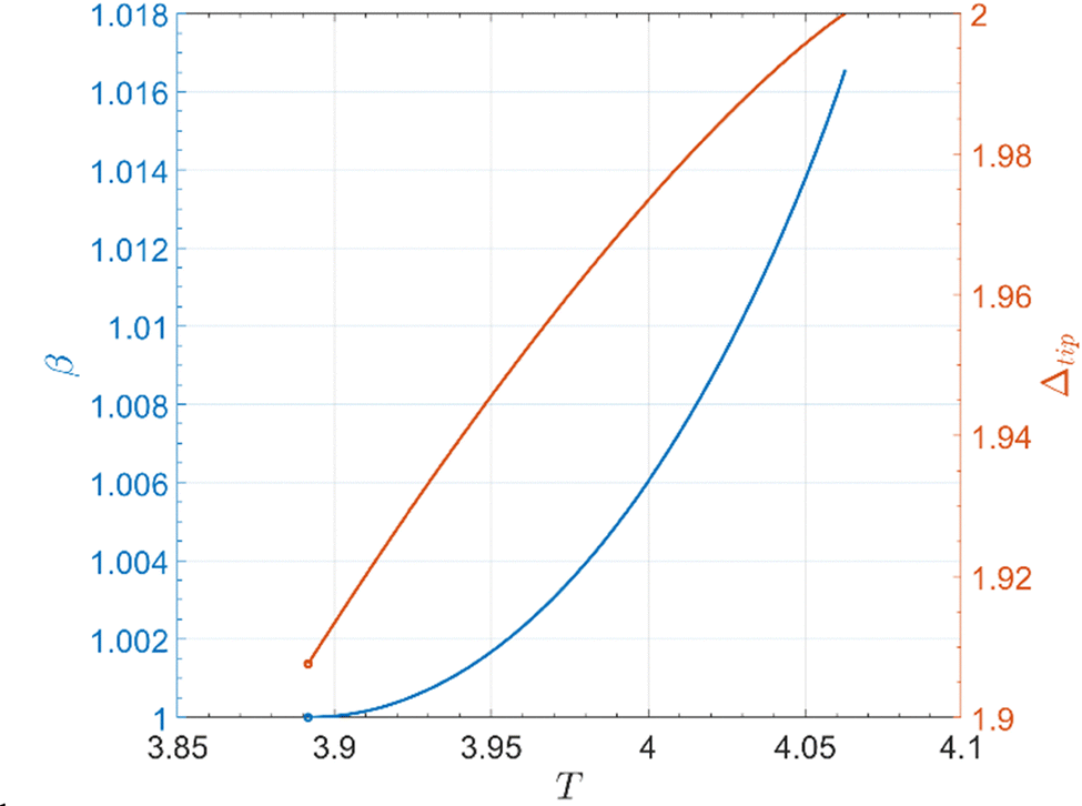
Eqn (43a) is solved numerically using ode45 in Matlab using the initial condition (43b). In these calculations, we chose different values of α < α* so crack initiation occurs on the ascending branch at T = TI and is followed by stable growth. The initiation time is determined by solving (22). We stop the program if Δtip reaches its maximum value ϕmax, i.e., at T = Tmax. Fig. 5 below shows the result for α = 0.5 < α* = 1.7071, with β0 = 1, ηmax = 1 and ϕmax = 2. The blue line in this figure is the normalized crack length β versus time. It shows that the crack reaches a constant velocity shortly after initiation. For this value of α (fairly slow loading rate), the crack remains on the ascending branch for all times, that is, ϕmax is never reached (see the red line which plots Δtipversus time).
 |
| | Fig. 5 Normalized crack length β (blue line) and Δtip (red line) versus normalized time T for α = 0.5 < α* = 1.7071. Simulations used β0 = 1, ηmax = 1, and ϕmax = 2. The black dashed line is the linear fit of β(T) with slope 0.1879. | |
The numerical result in Fig. 5 shows that Δtip is practically constant for large T, and in this regime, β ≈ b + ωT where ω and b are constant. Since 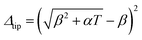 , it is possible for it to approach a constant at large T if β2 ≫ αT so that
| | 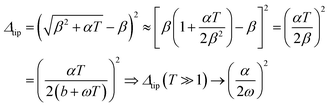 | (44) |
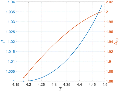
In Fig. 5, the fitted slope gives ω = 0.1879, and with α = 0.5, the asymptotic value of Δtip is predicted to be approximately 1.77, which is consistent with the numerical result of 1.75. As expected, crack growth remains on the ascending branch and reaches steady state as long as α < ηmax, which is consistent with our numerical results, shown in Fig. 5 and 6 (α = 0.9). Plots with other values of loading rates are similar and are given in ESI.†
 |
| | Fig. 6 Normalized crack length β (blue line) and Δtip (red line) versus normalized time T for α = 0.9 < α* = 1.7071. Simulations used β0 = 1, ηmax = 1, and ϕmax = 2. Note α = 0.9, slightly below ηmax = 1. | |
The situation is different for α* > α > ηmax. For this case, our analysis (see Appendix) shows that Δtip will reach ϕmax, so it is possible for the crack to reach the descending branch. Fig. 7 and 8 show the simulation results with α = 1.1 and 1.2 respectively.
 |
| | Fig. 7 Normalized crack length β (blue line) and Δtip (red line) versus normalized time T for α = 1.1 < α* = 1.7071. Simulations used β0 = 1, ηmax = 1, and ϕmax = 2. Note α = 1.1, slightly above ηmax = 1. | |
 |
| | Fig. 8 Normalized crack length β (blue line) and Δtip (red line) versus normalized time T for α = 1.2 < α* = 1.7071. Simulations used β0 = 1, ηmax = 1, ϕmax = 2. | |
Note that the crack velocity starts at zero and keeps increasing until ϕ reaches its maximum value, which is 2 in our simulations. However, our attempt to solve the differential equation on the descending branch fails – we cannot find equilibrium solution for (43a) on the descending branch. Specifically, in the first step of the solution process with the initial condition obtained from the numerical solution on the ascending branch at Δtip = ϕmax, we find that the LHS of eqn (43a) is larger than ϕmax which is impossible. This indicates that the solution on this branch is unstable, and that it is necessary to include inertia effects to balance energy.
Discussion and summary
In many soft polymer-based materials, viscoelastic losses during fracture propagation tests occur across various length scales. These include: the structural scale of sample deformation, the local scale of the process zone near the crack tip where bulk dissipation occurs, and the molecular scale where the polymer network is heavily stretched and damaged. While the structural scale depends on the sample geometry and loading, and can be modeled by continuum mechanics, both local and molecular energy dissipation can sometimes be modeled using cohesive zones. For instance, in adhesive tapes, the viscoelastic stretching of the confined adhesive into a fibrillar region can be represented by a rate-dependent cohesive zone acting between the elastic backing and the substrate. In glassy polymers, the localized visco-plastic process zone during small-scale yielding can similarly be modeled by a rate-dependent cohesive zone in an elastic sample with a propagating crack. In elastic polymer networks such as rubber and hydrogels, the molecular stretching and damage of the polymer network often result in rate-dependent fracture energy, which can also be modeled using a rate dependent cohesive zone in a soft elastic sample.
The classical understanding of crack propagation stability, which links structural characteristics such as (dG/dA < 0, A is the crack area) with material properties (dΓ/dv > 0), is overly simplistic as it only applies to steady-state conditions. It fails to explain phenomena like crack initiation and stick-slip dynamics. Key features, such as (1) whether slow fracture propagation occurs before rapid unstable crack growth (slip), (2) the dependence of the critical strain energy release rate for unstable rapid crack growth (slip) on the loading rate in elastic samples, and (3) delayed fracture initiation after static loading, cannot be fully captured or even qualitatively described by the classical approach.
The classical approach for predicting crack propagation under time-variable loading involves evaluating the strain energy release rate, G(c,uA) as a function of crack length and external loading, and using the steady-state toughness function, Γ(v), to predict the crack propagation rate. This yields a differential equation for quasi-static crack growth. While this method works when representing the crack front as a mathematical line with an energy sink Γ, it overlooks the finite length scale L of the cohesive zone at the crack front. This length scale introduces a characteristic timescale t* ≡ L/v which determines how long it takes to reach steady-state after changes in loading conditions. Thus, the classical approach is only valid if loading changes occur over timescales longer than t*. However, this is not the case during crack initiation under ramp loading or in stick-slip dynamics, where the loading time is comparable to or shorter than t*. The fracture energy function alone cannot capture these non-steady-state effects. Our work demonstrates that using a rate-dependent cohesive zone model provides a more accurate physical description of these effects. It also allows us to quantify critical loading rates where transitions between different phenomena occur, considering both crack propagation properties and the structural characteristics of the sample.
To provide a concise analytical description of the kinematics of crack propagation in a rate-dependent cohesive zone under time-dependent loading, we developed a model based on the zero-angle peeling of adhesive tape, also known as the shear lag test. We selected the simplest form of a rate-dependent cohesive zone to capture the general behavior of fracture energy: increasing with the local loading rate, reaching a maximum, and then decreasing. This was implemented using a Dugdale-like visco-plastic model with constant cohesive stress τ0 and rate-dependent maximum elongation δc.
The set of analytical expressions and differential equations, combined with numerical simulations, enabled us to describe different stability regimes of steady-state crack propagation and to illustrate the viscoelastic effects during non-steady-state loading. Specifically, we identified several regimes of crack propagation kinetics when a static crack is loaded at a constant velocity:
(1) At very low loading rates, crack propagation begins at a low velocity after a delay and gradually accelerates to reach steady-state conditions.
(2) At moderate loading rates, crack propagation starts slowly, similar to the low-rate case, but then the velocity continuously increases until a critical velocity is reached. Beyond this point, the strain energy release rate becomes critical, and the crack becomes unstable, rapidly accelerating to dynamic conditions. We remark that in these conditions, the critical strain energy release rate is independent of the sample loading rate.
(3) At high loading rates, no crack propagation occurs initially during loading. Once the unstable region is reached, sudden dynamic crack propagation occurs after the critical strain energy release rate is achieved, which decreases with increasing loading rate.
These different kinetic regimes demonstrate how the model captures the transition between stable and unstable crack propagation, driven by both loading rate and the viscoelastic response of the material. When applied to stick-slip dynamics, this model helps explain why, for some materials and geometries (such as PSA and epoxy resin), the amplitude of stick-slip oscillations depends on the loading rate, while for others (such as PMMA), it does not. The latter behavior is the only one predicted by classical models. Although the present simplified model cannot be directly applied to these experimental configurations, some quantitative links can be made with the fracture propagation regimes in previously published experimental data. Concerning PMMA, the characteristic velocity of the toughness peak is 1 cm s−1, the cohesive zone has typical length of 30 μm and the characteristic time to cross it is thus 3 ms.7 During any kind of macroscopic fracture tests leading to stick-slip the loading time for each stick-slip cycle is longer than 10 s, and is thus much larger than 3 ms.8 The loading rate is thus systematically slower than the critical value for unstable initiation, and the fracture will systematically reach steady-state (at low loading rate) or stick-slip with constant maximum toughness (at the highest achievable loading rates).2 Concerning epoxy resins, the characteristic velocity of the toughness peak is about 1 nm s−1, which is 7 orders of magnitude smaller than for PMMA.8 The typical length of the cohesive zone is 10 μm, and the characteristic time to cross it is thus several hours.8 During typical loading macroscopical fracture tests in epoxy the loading time before each stick-slip event ranges from seconds to minutes and is thus much shorter that hours. The loading rate is thus systematically faster than the critical value for unstable initiation, and the fracture will thus systematically start in an unstable condition, and thus present a toughness that decreases with the loading rate as observed in experiments.3 Concerning PSA, the characteristic velocity of the toughness peak is about 1 cm s−1, the cohesive zone has typical length of 100 μm and the characteristic time to cross it is thus 10 ms.14 During typical stick-slip crack propagation the order of magnitude of the frequency of stick-slip cycles is 100 Hz, so the typical duration of the reloading phases is 10 ms,6 which is comparable with the characteristic time to cross the process zone. This explains why typical experimental data present a transition from a constant maximum toughness at slow loading rates, to a decreasing toughness at higher loading rates, which is consistent with our modeling.1
There is one more stick-slip dynamics regime that escapes a sound interpretation using the classical approach. When the sample loading rate is so fast that the critical strain energy release rate for unstable crack initiation decreases close to the lower limit, the amplitude of the stick-slip cycles becomes very weak in experiments, and the crack length increment in each cycle can decrease to less than the cohesive zone length. Under these circumstances the entire slip phase occurs under non-steady-state conditions and its dynamics can no longer be described by Fig. 1, as is generally the case for large amplitude stick-slip. Although this regime is frequently reported as stable crack propagation,3 since the force fluctuations are very weak, and the crack increments are barely noticeable, the propagation is strictly unstable as long as the slope of the curve is weak but still negative and should be properly described by an extension of the present model to account for dynamic effects. For example, in the present shear loading configuration, the elasto-dynamic equation of the tight backing could be implemented in order to describe the generation of propagating elastic waves due to sharp variations of the crack propagation velocity during stick-slip or even the excitation of global vibrational modes of the backing when the stick-slip frequency matches the resonance frequency of the tight backing.
Finally, although our mathematical derivations are based on simplified assumptions, the model incorporates all fundamental aspects of rate-dependent crack propagation. We believe our model is broadly applicable across various materials and scenarios, even if more complex mathematical expressions may be needed in specific cases. These findings highlight the critical role of rate-dependent crack propagation, and they should be considered by researchers modeling crack propagation kinetics under non-steady-state conditions.
Data availability
There are no experiments, and all calculations are analytical, and derivations are given in the appendix.
Conflicts of interest
There are no conflicts to declare.
Appendices
Initiation time
First, for a fixed crack length β and loading rate α, the LHS of (22), i.e., 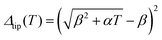 is a monotonically increasing function of T. For short times,
  , i.e., Δtip(T) increases from T = 0 quadratically. For very long times, Δtip(T) ∼ αT, it is linear in time with slope α.
Next, we consider the RHS of (22). There are two cases: α ≤ ηmax and α > ηmax.
For the case of α ≤ ηmax, since
| |  | (A1.1) |
for all
T, it is impossible for the RHS of
(22),
i.e.,

to reach
ϕmax. This means that the value of the RHS of
(22) is confined to the ascending branch of
ϕ. Since

is a monotonic increasing function of
T starting at 0 at
T = 0 and increases to its limiting value of
α as
T → ∞, the RHS of
(22) increases from 1 to
ϕ(
α) as
T → ∞. Note the LHS of
(22),
i.e.,

increases monotonically from 0 at
T = 0 to infinity as
T approaches infinity. The last two sentences imply that the curve associated with the LHS (
 versus T
) must lie below the curve associated with RHS for sufficiently short times; however, for long times, the situation is reversed. Since both the LHS and RHS of
(22) are monotonic increasing functions, there must exist a unique value of
T =
TI such that the two curves intersect,
i.e., RHS = LHS, resulting in satisfaction of the initiation condition
(22). This shows that for
α ≤
ηmax, initiation occurs on the ascending branch. This case is illustrated in
Fig. 9.
 |
| | Fig. 9 Schematic illustration of case 1 where α ≤ ηmax for fracture initiation. (a) Blue curve is the RHS of (22), i.e., ϕ while red curve is the LHS, i.e., Δtip, the intersection gives the initiation time. (b) Schematic plot of the shear response function ϕ showing relation between α, ηmax and α*. Plots not to scale. | |
Next, consider the 2nd case where α > ηmax. For this case, the RHS of (22), when plotted against T, reaches ϕmax at some time Tmax(α), i.e., this occurs when
| |  | (A1.2) |
Next, consider the LHS of
(22),

, there are three possibilities:
Δtip(
T =
Tmax) <
ϕmax,
Δtip(
T =
Tmax) >
ϕmax and
Δtip(
T =
Tmax) =
ϕmax.
In the first scenario: Δtip(T = Tmax) < ϕmax, because of α > ηmax, the RHS of (22) takes value on the descending branch of  for T > Tmax(α). On the other hand, the curve associated with the LHS increases monotonically from 0 to ∞, the two curves must intersect and since Δtip(T = Tmax) < ϕmax, this intersection must takes place on the descending branch of ϕ to the right of Tmax(α), i.e., TI > Tmax(α). This situation is shown schematically in Fig. 10(e) and (f).
 |
| | Fig. 10 Schematic illustration of case 2 where α > ηmax for fracture initiation. In (a), (c) and (e) blue curve is the RHS of (22), i.e., ϕ, and red curve is the LHS, i.e., Δtip, the intersection gives the initiation time. (b), (d) and (f) Plot the shear response function ϕ showing relation between α, ηmax, and α*. (a) and (b) ηmax < a < a*; (c) and (d) α = α*; (e) and (f) α > α* plots not to scale. | |
The condition Δtip(T = Tmax) < ϕmax can be written as (using (A1.2) and the definition of Δtip)
| |  | (A1.3) |
(A1.3) can be rewritten as (see
(23))
| |  | (A1.4) |
This shows that for α* < α, initiation must take place on the descending branch.
For the 2nd scenario where Δtip(T = Tmax) > ϕmax, the LHS of (22) must intersect the ascending branch of  to the left of Tmax(α), i.e., Tmax(α) > TI. Using the same idea, it is easy to show that Δtip(T = Tmax) > ϕmax is equivalent to α* > α. This situation is shown schematically in Fig. 10(a) and (b).
Finally, the third case corresponds to α = α*, the intersection occurs at ϕ = ϕmax and  as shown in Fig. 10(c) and (d). Note that
| |  | (A1.5a,A1.5b) |
Eqn (A1.5a, b) are equivalent to (23) and (24).
To summarize: if α < α*, then initiation occurs on the ascending branch. If α > α*, then initiation occurs on the descending branch. If α = α*, the initiation occurs at the peak with initiation time given by (24).
Finally, we note
| |  | (A1.6a,A1.6b) |
The validity of (A1.6a, b) can be established by substituting (A1.6a, b) into the RHS of (22) and noting that this side goes to 1 as α → 0+, ∞. It is then straightforward to show that LHS of (22) is consistent with these expressions.
Next, we show that TI(α) is a strictly monotonically decreasing function of α for α > α*. Since we already proof that a unique root of  exist, we compute
  using implicit differentiation, i.e.,
| |  | (A1.7a) |
where
| |  | (A1.7b) |
| |  | (A1.7c) |
Note that the term inside the square bracket in
(A1.7b) is always positive and less than 1. On the descending branch, where
ϕ′ < 0, both ∂
F/∂
α and ∂
F/∂
T are positive. Since the root for
α >
α* must occur on the descending branch,
.
Nomenclature (English alphabets followed by greek; in alphabetical order)
|
c
| Length of interface crack or the length of the peel arm, see in Fig. 2 |
|
c
0
| Crack length set at t = 0 for steady state |
|
C
|
 normalized interface crack length normalized interface crack length |
|
C
ss
| Steady-state normalized crack length |
|
Ċ
ss
| Steady-state normalized crack velocity |
|
E* | Plane strain modulus of the elastic backing layer |
|
F
| Force applied to the peel arm |
|
F
ss
| Constant peel force at the end of peel arm for steady-state crack growth |
|
G
| Strain energy release rate |
|
h
| Elastic backing layer thickness, see in Fig. 2 |
|
l
| Cohesive zone length, see in Fig. 2 |
|
L
|
 normalized cohesive zone length normalized cohesive zone length |
|
L
ss
| Steady-state normalized cohesive zone length |
|
s
| ≡ (ϕmax − 1)/ηmax positive slope of ϕ(η) used in piece-wise linear shear response function, eqn (25) |
|
t
| Time |
|
T
|
 normalized time normalized time |
|
T
I
| Normalized crack initiation time, eqn (22) |

| Critical initiation time corresponding to critical normalized velocity,  |
|
u
| Displacement of the elastic backing layer |
|
u
A
| ≡ u(x = 0)) horizontal displacement applied to the end of elastic layer, see in Fig. 2 |
|
U
A
| ≡ uA/δ0 normalized applied displacement to the peel arm |
|
v
| Crack velocity |
|
v
ss
| Constant peel velocity, or crack growth rate in steady-state crack growth |
|
V
ss
| Normalized steady-state crack velocity, see in eqn (29b) |
|
x
| Horizontal coordinate, with x = 0 located at right end of the elastic layer where displacement is applied to, Fig. 2 |
|
X
|
 normalized horizontal coordinate normalized horizontal coordinate |
|
α
| Normalized constant peeling (loading) velocity, eqn (18) |
|
α*
| Critical normalized loading velocity determining whether fracture initiation occurs on the ascending or descending branch, eqn (23) |
|
β
|
 , normalized crack length, eqn (16) , normalized crack length, eqn (16) |
|
β
0
| ≡ β(T = TI), initial normalized crack length |
|
Γ
| Velocity dependent fracture toughness |
|
Γ
0
| = τ0δ0, interfacial toughness at zero slip rate of Dugdale–Barenblatt (DB) model |
|
Γ
c
| = τ0δc, interfacial toughness of DB model |
|
δ
| Shear displacement jump or slip across the backing/substrate interface |
|
δ
0
| Critical slip at zero slip rate in DB model, see eqn (2) |
|
δ
c
| Rate dependent critical slip above which the interface fails, see eqn (2) |
|
δ
tip
| ≡ δ(x = −c) slip at the tip of crack |

| Slip rate |

| Characteristic slip rate in DB model, eqn (2) |
|
Δ
| ≡ δ/δ0 normalized slip displacement |
|
Δ
ss
|
Δ
tip for steady-state crack growth |
|
Δ
tip
| ≡ Δ(X = −C) = δtip/δ0 normalized slip at the tip of crack |

|
 material time derivative of normalized slip, eqn (20c) material time derivative of normalized slip, eqn (20c) |

|
 time derivative of normalized slip at crack tip time derivative of normalized slip at crack tip |
|
ε
A
| Tensile strain in the peel arm |
|
η
|
 , normalized slip rate , normalized slip rate |
|
η
max
|
ϕ(ηmax) = ϕmax |
|
Λ
| Difference between normalized energy release rate and normalized intrinsic toughness, eqn (38) |
|
ξ
| ≡ c0 + x + vsst coordinate with origin located at moving crack tip |
|
Ξ
|
 normalized ξ coordinate (moving frame) normalized ξ coordinate (moving frame) |
|
σ
| Uniaxial tension in elastic layer |
|
τ
| Interfacial shear stress |
|
τ
0
| Constant shear stress value used in DB model, eqn (2) |
|
ϕ
| Shear response function used in this work, depends only on  |
|
ϕ
max
| Maximum value of ϕ |
|
Φ
| General form of shear response function which depends on both δ and  , eqn (1) , eqn (1) |
|
ω
| Normalized crack length β growth rate, i.e.,  at large time at large time |
Acknowledgements
Chung-Yuen Hui and Xuemei Xiao acknowledge the support from the National Science Foundation, CMMI-1854572. Matteo Ciccotti acknowledges the support from the ANR grant VITRIPSA (ANR-21-CE06-0025).
References
- M. Barquins, B. Khandani and D. Maugis, C. R. Acad. Sci., Ser. II, 1986, 303, 1517–1519 Search PubMed
 .
.
- M. L. Hattali, J. Barés, L. Ponson and D. Bonamy, Mater. Sci. Forum, 2012, 706–709, 920–924 CAS .
- A. J. Kinloch, D. L. Maxwell and R. J. Young, J. Mater. Sci., 1985, 20, 4169–4184 CrossRef CAS .
-
D. Maugis and M. Barquins, in Adhesion 12, ed. K. W. Allen, Springer Netherlands, Dordrecht, 1988, pp. 205–222 Search PubMed .
- D. C. Hong and S. Yue, Phys. Rev. Lett., 1995, 74, 254–257 CrossRef CAS PubMed .
- M. Ciccotti, B. Giorgini and M. Barquins, Int. J. Adhes. Adhes., 1998, 18, 35–40 CrossRef CAS .
-
W. Döll, in Crazing in Polymers, ed. H. H. Kausch, Springer, Berlin, Heidelberg, 1983, pp. 105–168 Search PubMed .
- Y. Nziakou, M. George, G. Fischer, B. Bresson, M. Tiennot, S. Roux, J. L. Halary and M. Ciccotti, Soft Matter, 2022, 18, 793–806 RSC .
- R. Villey, C. Creton, P.-P. Cortet, M.-J. Dalbe, T. Jet, B. Saintyves, S. Santucci, L. Vanel, D. J. Yarusso and M. Ciccotti, Soft Matter, 2015, 11, 3480–3491 RSC .
- A. Needleman, J. Appl. Mech., 1987, 54, 525–531 CrossRef .
- M. Elices, G. V. Guinea, J. Gómez and J. Planas, Eng. Fract. Mech., 2002, 69, 137–163 CrossRef .
- J. G. Williams and H. Hadavinia, J. Mech. Phys. Solids, 2002, 50, 809–825 CrossRef .
- C. Y. Hui, A. Ruina, R. Long and A. Jagota, J. Adhes., 2011, 87, 1–52 CrossRef CAS .
- R. Villey, P.-P. Cortet, C. Creton and M. Ciccotti, Int. J. Fract., 2017, 204, 175–190 CrossRef .
- S. Ponce, J. Bico and B. Roman, Soft Matter, 2015, 11, 9281–9290 RSC .
|
| This journal is © The Royal Society of Chemistry 2025 |
Click here to see how this site uses Cookies. View our privacy policy here. 
 *ab,
Xuemei
Xiao
a and
Matteo
Ciccotti
*ab,
Xuemei
Xiao
a and
Matteo
Ciccotti


 is the time rate of shear displacement or slip rate. Eqn (1) applies to an interface continuum point, so δ and
  can vary spatially and temporally. Motivated by the mechanics of fibril stretching described above, the shear stress response function Φ has the following characteristics: the work to debond the interface first increases with the slip rate, reaches a maximum at some rate, then decreases to some constant value afterward.

 , δ0 are material constants.
  is a characteristic slip rate and δ0 is the critical slip at zero slip rate. In this model the energy required to debond a unit area of the interface, or the interfacial toughness is Γc = τ0δc. In the classical DB model, δc is independent of slip rate, but here we assume δc depends on the slip rate through the response function ϕ(η) where
  . Note by definition,
 . (a) Shows a general function of ϕ(η) which starts at ϕ(η = 0) = 1, monotonically increases to ϕmax at η = ηmax and then monotonically decreases to 1 as η → ∞. (b) Is the piecewise-linear function we use in this paper for analytical analysis in the section called fracture initiation.


 and displacements by δ0


 .
.


 . From here on, we will refer to either C or β as the normalized crack length.
 , is applied to the peel arm at x = 0, where α is the normalized peel rate, i.e.,


 in (20b) depends on both the crack motion and the loading rate. Specifically, using (12),
 from dΔtip(T)/dT, we denote
  with a dot. Only in the special case of a stationary crack where dC/dT = 0, does
  . Note for the special case of steady-state crack growth, dΔtip(T)/dT = 0 and
  .
.
 are independent of time, the local slip rate is obtained by setting dC/dT = 0 in (20c) and evaluating
  using (19), this results in

 . Also, when crack growth rate is zero, (21b) reduces to (21a).
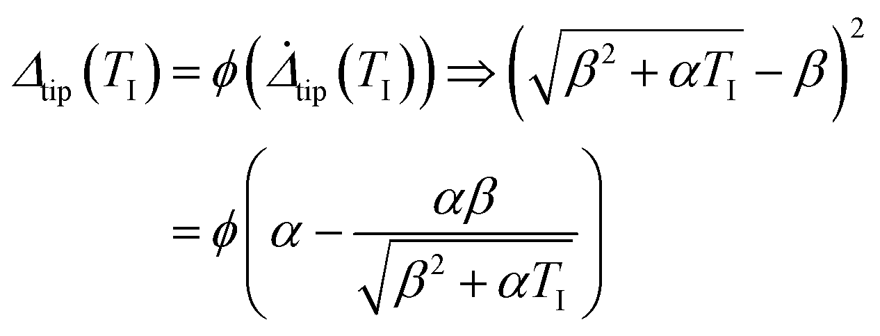


 as solid lines, and the RHS of (22), i.e.,
  as dash-dot lines, both plotted against the normalized time T for different values of α. For each value of α, the RHS and LHS of (22) generate two curves. Note that the LHS of (22) is a monotonically increasing function of T with increasing slope whereas the RHS of (22) increases, reaches a maximum, and then decreases. As a result, the two curves intersect at a single point, which gives the initiation time TI. In Fig. 4, we use β = β0 = 1, ϕmax = 4, and ηmax = 1. The critical loading rate α* = 3/2 with
  is used as a reference. An interesting result shown in Fig. 4 is that the initiation time decreases with increasing α.
 (solid lines) and
 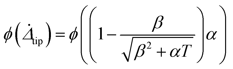 (dash-dot lines) are plotted against normalized time T for 6 different normalized loading rates α. The intersection of these curves, indicated by a circle, gives the initiation time TI. (For α = 0.375, the initiation time TI exceeds beyond the maximum plotted time of 10 and is therefore not displayed.) The curves are generated using β = β0 = 1, ϕmax = 4, and ηmax = 1. For this case, the critical loading rate is α* = 1.5. Consistent with theory, initiation occurs on the ascending/descending branch for α < α*/α > α* respectively.


 in (34b) can be obtained using steady-state condition (26) and is


 , (40) is satisfied, so steady-state crack growth is always unstable on this branch.
 . Note when Δss = ϕmax, the maximum velocity for stable crack growth is reached, which is


 , so it is a different normalization of the crack length.

 , it is possible for it to approach a constant at large T if β2 ≫ αT so that


 is a monotonically increasing function of T. For short times,
  , i.e., Δtip(T) increases from T = 0 quadratically. For very long times, Δtip(T) ∼ αT, it is linear in time with slope α.

 to reach ϕmax. This means that the value of the RHS of (22) is confined to the ascending branch of ϕ. Since
  is a monotonic increasing function of T starting at 0 at T = 0 and increases to its limiting value of α as T → ∞, the RHS of (22) increases from 1 to ϕ(α) as T → ∞. Note the LHS of (22), i.e.,
  increases monotonically from 0 at T = 0 to infinity as T approaches infinity. The last two sentences imply that the curve associated with the LHS (
 versus T) must lie below the curve associated with RHS for sufficiently short times; however, for long times, the situation is reversed. Since both the LHS and RHS of (22) are monotonic increasing functions, there must exist a unique value of T = TI such that the two curves intersect, i.e., RHS = LHS, resulting in satisfaction of the initiation condition (22). This shows that for α ≤ ηmax, initiation occurs on the ascending branch. This case is illustrated in Fig. 9.


 , there are three possibilities: Δtip(T = Tmax) < ϕmax, Δtip(T = Tmax) > ϕmax and Δtip(T = Tmax) = ϕmax.
 for T > Tmax(α). On the other hand, the curve associated with the LHS increases monotonically from 0 to ∞, the two curves must intersect and since Δtip(T = Tmax) < ϕmax, this intersection must takes place on the descending branch of ϕ to the right of Tmax(α), i.e., TI > Tmax(α). This situation is shown schematically in Fig. 10(e) and (f).

 to the left of Tmax(α), i.e., Tmax(α) > TI. Using the same idea, it is easy to show that Δtip(T = Tmax) > ϕmax is equivalent to α* > α. This situation is shown schematically in Fig. 10(a) and (b).
 as shown in Fig. 10(c) and (d). Note that
 exist, we compute
  using implicit differentiation, i.e.,


 .
.
 normalized interface crack length
 normalized cohesive zone length
 normalized time

 normalized horizontal coordinate
 , normalized crack length, eqn (16)


 material time derivative of normalized slip, eqn (20c)
 time derivative of normalized slip at crack tip
 , normalized slip rate
 normalized ξ coordinate (moving frame)
 , eqn (1)
 at large time