
 Open Access Article
 This Open Access Article is licensed under a
 Creative Commons Attribution 3.0 Unported Licence
Collective dynamics of intelligent active Brownian particles with visual perception and velocity alignment in 3D: spheres, rods, and worms†
Zhaoxuan
Liu
 and
Marjolein
Dijkstra
*
and
Marjolein
Dijkstra
*
Soft Condensed Matter & Biophysics Group, Debye Institute for Nanomaterials Science, Utrecht University, Princetonplein 1, 3584 CC Utrecht, The Netherlands. E-mail: m.dijkstra@uu.nl
First published on 22nd January 2025
Abstract
Many living systems, such as birds and fish, exhibit collective behaviors like flocking and swarming. Recently, an experimental system of active colloidal particles has been developed, where the motility of each particle is adjusted based on its visual detection of surrounding particles. These particles with visual-perception-dependent motility exhibit group formation and cohesion. Inspired by these behaviors, we investigate intelligent active Brownian particles (iABPs) equipped with visual perception and velocity alignment in three dimensions using computer simulations. The visual-perception-based self-steering describes the tendency of iABPs to move toward the center of mass of particles within their visual cones, while velocity alignment encourages alignment with neighboring particles. We examine how the behavior varies with the visual cone angle θ, self-propulsion speed (Péclet number Pe), and the interaction strengths of velocity alignment (Ωa) and visual-based self-steering (Ωv). Our findings show that spherical iABPs form dense clusters, worm-like clusters, milling behaviors, and dilute-gas phases, consistent with 2D studies. By reducing the simulation box size, we observe additional structures like band-like clusters and dense baitball formations. Additionally, rod-like iABPs form band-like, worm-like, radiating, and helical structures, while iABP worms exhibit band-like, streamlined, micellar-like and entangled structures. Many of these patterns resemble collective behaviors in nature, such as ant milling, fish baitballs, and worm clusters. Advances in synthetic techniques could enable nanorobots with similar capabilities, offering insights into multicellular systems through active matter.
1 Introduction
Active matter consists of entities that extract energy from their environment and convert it into directed motion. Nature offers many examples of active matter systems, from bird flocks and buffalo herds to bacteria, chasing white blood cells, cancerous tumor growth, and embryogenesis. Many living systems exhibit collective behaviors that resemble flocks or swarms.1 These groups can display unique patterns, like ant milling,2 where ants continuously circle around a specific point until they die from exhaustion, a phenomenon referred to as the ‘circle of death’. Reindeer can form cyclones, penguin huddles can crystallize and undergo jamming–unjamming transitions,3 and sheep display intricate flocking patterns.4 While many of these behaviors occur in two-dimensional environments, such as on land or ice, aquatic and aerial settings offer opportunities for three-dimensional behaviors. For instance, fish form baitballs5—dense spherical aggregates—as a defense mechanism against predators. Fire ants build bridges and rafts to navigate their surroundings,6,7 and blackworms exhibit rapid transitions from tangled blobs to untangled states for survival.8,9 These collective behaviors are crucial for activities like finding food and avoiding predators, emerging naturally from individual responses to others in the group without centralized control.The study of such phenomena offers valuable insights not only into biological processes but also into the design of artificial systems that mimic these behaviors. Over the past two decades, a wide variety of self-propelled colloidal particles has been synthesized, including magnetic-bead-based colloids that mimic artificial flagella,10 catalytic Janus particles,11–14 laser-heated metal-capped particles,15 light-activated catalytic colloidal surfers,16 and platinum-loaded stomatocytes,17 as well as robotic systems spanning scales from micrometers to centimeters. Inspired by nature, researchers have developed models to simulate collective dynamics, where emerging patterns rely on physical interactions and nonreciprocal information exchanges, such as visual-perception-based self-steering and velocity alignment. These interactions and communication processes are key to the formation of swarms and flocks. Motion alignment and group cohesion are fundamental characteristics of these collective behaviors, and various models have been proposed to understand how these processes give rise to the intricate structures observed in nature.
One of the simplest models that describe collective motion in systems of self-propelled particles is the Vicsek model proposed in 1995.18 In this model, point particles move at a constant speed and update their velocity by aligning with the average direction of neighbouring particles within a certain interaction range, while accounting for some noise. The large-scale collective behavior is purely driven by the velocity alignment among particles. The Vicsek model exhibits a phase transition from a disordered state, where particles move in random directions, to an ordered phase with polar order, where particles move in a coherent direction, upon increasing the particle density or reducing the noise, see also ref. 19.
The Boids model,20 introduced by Reynolds in 1987, describes the behavior of birds, also called boids, by incorporating three fundamental interaction rules: cohesion, separation, and alignment. These rules indicate that individuals strive to maintain proximity to their peers (cohesion), align their movement direction with the group (alignment), and avoid collisions with nearby individuals (separation). Additionally, the behavioural zonal model,21,22 introduced by Couzin in 2002, considers distinct interactions between individuals within three non-overlapping zones: repulsion at close distances, alignment with neighbors, and attraction toward others. This model exhibits collective behaviors such as swarming, milling, and groups with highly aligned motion.
It is important to highlight that the intricate patterns and structures arise from simple non-reciprocal interactions between individuals, meaning they violate Newton's third law of action-reaction symmetry. Remarkably, these complex behaviors emerge without any need for external control or coordination.
Another class of models involves active Brownian particles (ABPs), which mimick the behavior of self-propelled colloidal particles through self-propulsion forces and short-range repulsive excluded-volume interactions.23 In these systems, the shape of particles plays a crucial role in determining the collective behavior. Spherical ABPs often exhibit motility-induced phase separation (MIPS), where uniformly distributed particles undergo phase coexistence between a dense cluster and a dilute phase at sufficiently high self-propulsion speeds.24–27 In contrast, elongated ABPs exhibit distinct non-equilibrium behaviors, such as the formation of immobile dimers,28 motile clusters, swarms,29–31 and the suppression of motility-induced phase separation due to interparticle torques,32 emphasizing the impact of particle shape on the collective dynamics of active matter systems. Additionally, microswimmer models incorporating hydrodynamics reveal that these interactions result in increased repulsion between puller pairs and enhanced attraction between pusher pairs.33,34
In 2016, visual perception-based self-steering capabilities were introduced for active systems,35 revealing milling, cluster, worm, and dilute-gas structures. These capabilities were later incorporated into an ABP model.36 These models allow each particle to reorient its self-propulsion direction based on other particles within a predefined visual cone. These particles, referred to as intelligent active Brownian particles (iABPs), have since evolved with the integration of the Vicsek model,18 enabling iABPs to align their self-propulsion direction with that of their neighbors.37 As a result, these iABPs possess both visual perception-based self-steering and velocity alignment capabilities. It is also important to mention that these models can be realized experimentally.38–40 Recent studies on iABPs37 have demonstrated a range of collective structures, including milling, clusters, worms, and dilute-gas formations. However, these investigations have primarily been restricted to two-dimensional spaces with disk-like particles. Given that many animals navigate in three-dimensional environments and often have non-spherical bodies, there is a compelling case for expanding the study of iABPs to three-dimensional systems and aspherical shapes.
In this paper, we investigate three-dimensional intelligent active Brownian particles (iABPs) using computer simulations to explore their collective behaviors. We analyze these systems as a function of the vision angle θ, which affects the opening angle of the visual cone, the Péclet number Pe, which influences the self-propulsion speed, and the ratio Ωa/Ωv, which balances the velocity alignment and vision-based self-steering capabilities. Our results indicate that spherical iABPs form dense clusters, milling patterns, worm-like structures, and dilute-gas configurations, consistent with findings in 2D. By reducing the simulation box size, we also observe the emergence of band formations, dispersed clusters, and baitball structures. Additionally, rod-like iABPs exhibit band formations, worm-like, radiating, and helical structures, while iABP worms display band-like, streamlined, micellar-like and entangled configurations.
Some of these structures closely resemble real animal behaviors, such as ant milling, fish baitballs, and worm blobs, indicating that these models have the potential to predict collective animal behaviors. Furthermore, advancements in synthetic techniques could inspire the design of nanorobots and colloidal particles with similar capabilities. Recent research41,42 suggests that multicellular systems can also be understood through the framework of active matter. If the single-cell organisms that gave rise to multicellular creatures could sense light and velocity, the structures obtained in our model may provide valuable insights into the formation of multicellular systems.
This paper is organized as follows. In Section 2, we start our investigation with the collective dynamics of intelligent active Brownian particles (iABPs) with spherical shapes. In Section 3, we extend the iABP model to incorporate rod-like shapes using the Kihara potential. Finally, in Section 4, we connect spherical iABPs with ordinary Brownian particles to create iABP worms. We end with some conclusions in Section 5.
2 Intelligent active Brownian spheres
2.1 Model system
We consider a three-dimensional system of N intelligent active Brownian spheres at positions ri(t) and orientations ei(t) at time t, with i = 1,…,N. We employ the overdamped Langevin equation to describe the translational motion of each particle| ṙi = v0ei + βDtFWCAi + Γi, | (1) |
 , where UWCA is the Weeks–Chandler–Andersen (WCA) potential defined as
 | (2) |
The term Γi represents a stochastic force acting on each particle, characterized by a zero mean 〈Γi,α(t)〉 = 0 and second moment 〈Γi,α(t)Γj,β(t′)〉 = 2Dtδijδαβδ(t − t′), where α and β denote Cartesian coordinates.
The rotational motion of each particle is described by37
| ėi = Mvi + Mai + Λi × ei, | (3) |
Following ref. 37, the vision-based self-steering is described by
 | (4) |
 represents a normalization constant, and the summation runs over all particles j within the visual cone (VC). The visual cone is characterized by a range Rv and a vision angle θ, which sets the criterion for determining whether particle j lies within this cone by rij ≤ Rv and uij·ei ≥ cos
![[thin space (1/6-em)]](https://www.rsc.org/images/entities/char_2009.gif) θ with uij = (rj − ri)/|rj − ri|. These variables are depicted in Fig. 1. The vision-based self-steering adjusts a particle's self-propulsion direction in response to the positions of particles within its visual cone. As particles enter this cone, the particle reorients its self-propulsion direction toward the center of mass of the observed particles. The exponential term assigns higher weight to particles closest to the particle of interest, with a decay range of R0 = Rv/4. Here, we assume that the particle's vision is not hindered by other particles. Incorporating visual obstructions would require a more sophisticated model, which could limit the feasibility of simulating large system sizes. However, the exponential distance dependence in eqn (4) can be interpreted as a straightforward way to account for visual blocking, as it implies that visual perception is primarily dominated by the closest neighbors, effectively obscuring the view on particles farther away. Note that this equation originates from ref. 35 and was later modified in ref. 37.
θ with uij = (rj − ri)/|rj − ri|. These variables are depicted in Fig. 1. The vision-based self-steering adjusts a particle's self-propulsion direction in response to the positions of particles within its visual cone. As particles enter this cone, the particle reorients its self-propulsion direction toward the center of mass of the observed particles. The exponential term assigns higher weight to particles closest to the particle of interest, with a decay range of R0 = Rv/4. Here, we assume that the particle's vision is not hindered by other particles. Incorporating visual obstructions would require a more sophisticated model, which could limit the feasibility of simulating large system sizes. However, the exponential distance dependence in eqn (4) can be interpreted as a straightforward way to account for visual blocking, as it implies that visual perception is primarily dominated by the closest neighbors, effectively obscuring the view on particles farther away. Note that this equation originates from ref. 35 and was later modified in ref. 37.
 | ||
| Fig. 1 (a) A schematic illustration of two spherical intelligent active Brownian particles (iABPs), labeled i and j, positioned at ri and rj, with arrows indicating their self-propulsion directions, ei and ej, respectively. (b) A schematic of the visual cone (green) with a range of Rv and a vision angle θ, along with the polar-alignment sphere (grey), which has a radius of Ra. (c) Initial configuration of spherical iABPs. Particles are initially arranged on a simple cubic lattice (left panel) with self-propulsion directions randomly assigned (right panel). | ||
The velocity-alignment torque reads
 | (5) |
We employ Brownian dynamics simulations to explore the collective dynamics of intelligent active Brownian spheres. We numerically integrate the equations of motion in eqn (1) and (3) with a time step Δt = 10−5σ2/Dt. We run the simulations for 107 steps in total. For specific parameter sets, additional steps are conducted. The rotational diffusion coefficient is set to Dr = 3Dt/σ2. We initially perform simulations of N = 512 particles at a packing fraction of Φ = NVp/V = 6 × 10⁻⁵, where Vp = πσ3/6 denotes the volume of a single iABP, and V represents the total volume of the simulation box. The packing fraction is later increased to examine the effect of varying box sizes. All simulations are conducted using periodic boundary conditions. Furthermore, we set the radius of the polar-alignment sphere to Ra = 2σ, the characteristic decay range of the vision-based torque to R0 = 1.5σ, and the range of the visual cone to Rv = 6σ. In our simulations, we fix the strength of the vision-based self-steering Ωv = 102Dt/σ2, while adjusting the relative strength of the velocity alignment Ωa through the ratio Ωa/Ωv. We investigate the dynamic behavior of the system at varying self-propulsion speed v0, which is controlled through the Péclet number Pe = v0σ/Dt. The strength of the WCA potential is also adjusted with the Péclet number, using the relation ε/kBT = 1 + Pe. Additionally, we vary the vision angle θ from 0 to π. The simulations start with particles arranged in an 8 × 8 × 8 simple cubic lattice at the center of the box with a lattice spacing of σ. Each particle is initialized with a random self-propulsion direction to avoid directional bias, as illustrated in Fig. 1(c).
2.2 State diagram
To investigate the effects of velocity-alignment torque Ωv and vision angle θ on the dynamic behavior of intelligent active Brownian spheres (iABPs), we set the Péclet number to Pe = 70 and map out the state diagram by varying both the relative strength of velocity alignment to vision-based self-steering Ωa/Ωv, and the vision angle θ. Our initial analysis of the distinct dynamic behaviors of iABPs is primarily based on visual inspection of the resulting configurations, which provides an accurate representation since the structures are visually distinct. To offer a more rigorous characterization of the dynamic structures, we also introduce a quantitative approach using order parameters in Section 2.3 and validate the accuracy of the state diagrams through visual inspection. We summarize our observations in the state diagram shown in Fig. 2(a). We clearly identify four distinct regimes in the state diagram within the θ–Ωa/Ωv plane. At wide vision angles θ ≳ π/3 and low Ωa/Ωv ≲ 5, represented by the pink region, the particles form dense spherical clusters. Within these clusters, particles are oriented towards the center, leading to near-stationary behavior of the entire cluster as the self-propulsion forces balance out, see Fig. 4. In this regime, each iABP observes many neighbors within its visual cone and moves toward the center of mass of this particle cluster, resulting in dense aggregation driven by vision-based cohesion. Upon increasing Ωa/Ωv and thus the velocity alignment, the particles tend to align their velocities, forming motile worm-like structures where particles aggregate due to vision-based cohesion and move cohesively. These worm-like structures are observed for wide vision angles θ ≳ π/4 and high Ωa/Ωv ≳ 5, represented by the green region. Such structures consist of a leader particle with other particles following in alignment, as illustrated in Fig. 4. For sufficiently narrow vision angles θ ≲ π/4, represented by the yellow region, each iABP observes relatively few particles within its visual cone. The lack of vision-based cohesion causes the particles to become homogeneously distributed, resulting in a dilute-gas structure of motile particles (Fig. 4). Interestingly, at intermediate vision angles π/4 ≲ θ ≲ π/3 and moderate 0.5 ≲ Ωa/Ωv ≲ 1, represented by the blue region, we observe milling behavior. In this regime, the motile particles form rotating, doughnut-like configurations, which can be regarded as the leader particle of a worm-like structure looping back into the group, causing the worm-like swarm of particles to “bite its own tail,” as shown in Fig. 4, reminiscent of ant milling behavior.2 Video M1 (ESI†) provides an example for each structure. | ||
| Fig. 2 (a) State diagram of intelligent active Brownian spheres in the relative strength of the velocity alignment and vision-based self-steering Ωa/Ωv – vision angle θ plane at a packing fraction of Φ = 6 × 10⁻⁵, Péclet number Pe = v0σ/Dt = 70 and particle number N = 512. The pink region denotes dense clusters, the green region depicts worm-like structures, the blue region corresponds to milling behavior, and the yellow region denotes dilute-gas structures. (b) State diagram in the Péclet number Pe – vision angle θ plane at the same packing fraction and particle number with relative strength of the velocity alignment and vision-based self-steering Ωa/Ωv = 1. (c) A zoomed-in picture around the milling area in (b), highlighting the increase in milling size with higher values of Pe, floating particles are removed for Pe ≤ 90 to enhance the clarity. | ||
Intriguingly, the dense cluster at Ωa/Ωv = 5 and θ = π, located near the phase boundary between worm-like and dense cluster states, exhibits transient behavior, it can either form a moving dense cluster, unlike other dense clusters that tend to remain stationary, or take on a worm-like structure, as shown in Video M1 (ESI†). This behavior could stem from the inherent dynamic sensitivity of non-equilibrium systems near boundaries of different regimes in the state diagram, where small variations in initial orientations, and stochastic noise can lead to different final structures. Such transient dynamics is especially pronounced at Ωa/Ωv ⋍ 5, where distinguishing dynamic behaviors becomes increasingly challenging. Therefore, we will refrain from further investigations at Ωa/Ωv ⋍ 5.
Additionally, we investigate the effects of self-propulsion speed v0 and vision angle θ. Setting Ωa/Ωv = 1, we map out the state diagrams by varying Pe and θ, as shown in Fig. 2(b). We again observe four distinct regimes in Fig. 2(b). For sufficiently large vision angles θ ≳ π/4, dense cluster structures form, similar to our previous observations. Conversely, at small vision angles θ ≲ π/5, vision-based cohesion is too weak to favor aggregation, leading to a homogeneous dispersion of particles, i.e. dilute-gas structures. At intermediate vision angles π/5 ≲ θ ≲ 2π/5 and intermediate 30 ≲ Pe ≲ 100, milling structures are observed. As Pe increases (Pe ≳ 100) and thus the self-propulsion speed, the cluster regime narrows, and milling structures transition into worm-like structures. Conversely, decreasing Pe (Pe ≲ 20) increases diffusivity, enabling particles to escape the milling state.We observe that the state point near the boundary between milling and worm-like structures can transition between these two states over time, as shown in Video M1 (ESI†).
Importantly, our simulations offer strategies to prevent animals from forming milling structures (a.k.a. the ‘circle of death’ in the case of ant milling). Specifically, reducing the visual cone angle θ inhibits milling structures, leading particles to form dilute-gas states, while increasing θ promotes dense clustering, disrupting milling. Decreasing the Pe number, which lowers self-propulsion relative to diffusion, helps particles escape milling traps. Conversely, a higher Pe increases the milling size, leading to a thinner boundary. Eventually, the boundary becomes too thin to maintain the structure, causing it to break apart into several worm-like structures, as shown in Fig. 2(c). Besides, increasing velocity alignment strength Ωa reduces the frequency of turns, decreasing the likelihood of tail-biting events and effectively suppressing milling behavior. Some of these findings align with ref. 43, which shows that increasing noise and alignment strength can prevent the system from forming a milling structure.
In conclusion, our study reveals distinct collective behaviors based on vision angle θ, the ratio of velocity-alignment to vision-based self-steering interaction strengths Ωa/Ωv, and Pe number. Dense clusters emerge for wide vision angles θ ≳ π/3 and sufficiently small velocity-alignment interactions Ωa/Ωv ≲ 5, driven by vision-based cohesion that promotes aggregation. Dilute-gas structures dominate at narrow vision angles θ ≲ π/4, where the lack of vision-based cohesion prevents significant clustering. At vision angles π/4 ≲ θ ≲ π and strong velocity-alignment interactions Ωa/Ωv ≳ 5, we observe motile, worm-like swarms. These swarms can transition into milling structures at intermediate Péclet numbers 30 ≲ Pe ≲ 100 and intermediate 0.5 ≲ Ωa/Ωv ≲ 1. Interestingly, these findings align with 2D simulations,37 as the resulting structures appear to be 3D extensions of the 2D patterns. For instance, both 2D and 3D results exhibit milling, worm-like structures, and dense clusters that closely resemble the hexagonally close-packed (HCP) structures in 2D. However, we did not observe states with multiple aggregations, which were reported in 2D studies.
2.3 Characterization of dynamic states using order parameters
In Section 2.2, we presented state diagrams based on visual inspection of the dynamic behaviors of iABPs. Here, we introduce a quantitative approach using specifically designed order parameters and validate the accuracy of the state diagrams through visual inspection. To this end, we first determine the largest cluster in each configuration using a simple distance criterion rij < 2σ, where rij denotes the distance between particle i and j. To differentiate between the observed structures, we employ three distinct order parameters. We first calculate the polarization P defined as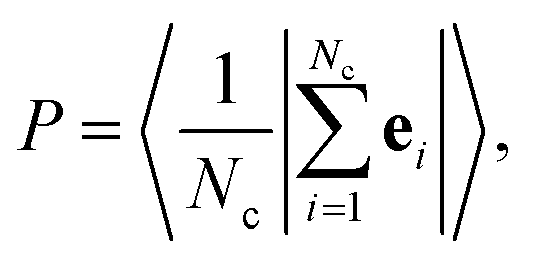 | (6) |
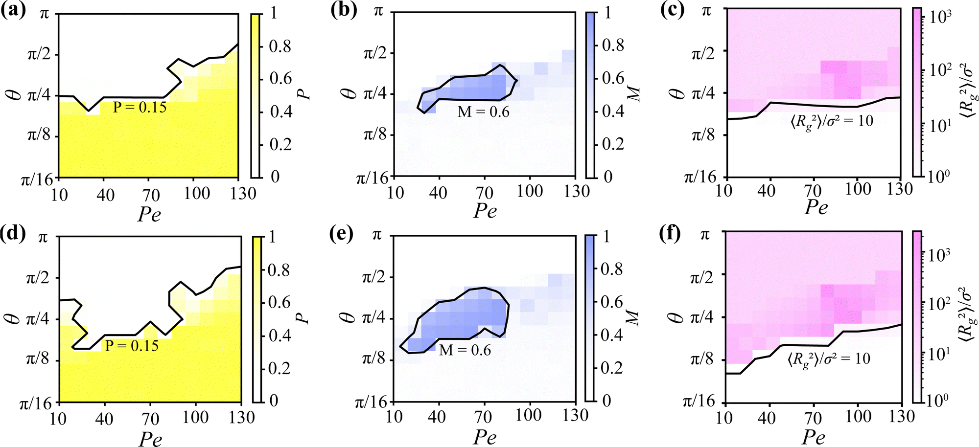 | ||
| Fig. 3 (a)–(c) Heat maps corresponding to Fig. 2(b), where each cell in the 13 × 13 grid directly represents a state point investigated through simulations. Colors represent the intensity of (a) the total polarization P, (b) the rotational polarization M, and (c) the radius of gyration 〈Rg2〉. Contour lines denote (a) P = 0.15, (b) M = 0.6, and (c) 〈Rg2〉/σ2 = 10. (d)–(f) Heat maps corresponding to the same set of parameters as (a)–(c), with the number of particles increased from N = 512 to N = 1000. | ||
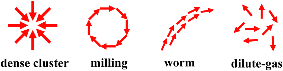 | ||
| Fig. 4 A schematic representation of the polarization (self-propulsion direction) across various structures. | ||
To quantify the rotational motion and identify milling structures, we employ the rotational polarization M, defined as
 | (7) |
Finally, we use the radius of gyration Rg to characterize the size of the largest cluster, defined as
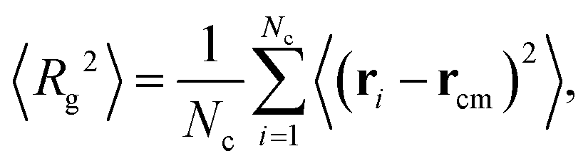 | (8) |
 is the center of mass of the cluster. The summation runs over all Nc particles in the largest cluster, and the averaging is performed over time after equilibration. Fig. 3(c) presents a heat map of 〈Rg2〉, with a contour line marking 〈Rg2〉 = 10σ2. This contour line effectively separates dilute structures, characterized by 〈Rg2〉 ≲ 10σ2, as they rarely form aggregates.
By comparing the heat maps in Fig. 3 with the state diagram in Fig. 2(b), we validate the accuracy of the state diagrams derived from visual inspection. The heat maps reveal that the polarization P effectively distinguishes milling and cluster structures from worm-like and dilute-gas structures, the rotational polarization M captures the rotational motion characteristic of milling structures, and the radius of gyration 〈Rg2〉 reliably identifies dilute-gas states due to their lack of aggregation. This quantitative analysis supports the classifications shown in the state diagrams.
To investigate the effect of system size, Fig. 3(d)–(f) present analyses using the same parameter sets as in Fig. 3(a)–(c), but with the particle number increased from 512 to 1000. The results show that while the overall distribution of regimes remains similar, the dilute-gas regime decreases noticeably, whereas the milling regime expands significantly. This indicates that a larger number of individuals is more prone to become trapped within milling structures.
2.4 Mean square displacement
To study the dynamics of the particles, we analyze the translational motion of the iABPs within each dynamic structure by measuring the mean square displacement (MSD) of the individual particles | (9) |
Here, the summation runs over all N particles, and the average is performed over different time windows. Note that the MSDs represent the average motion of individual particles, and not that of the aggregates. We present the MSD as a function of time for various structures of iABPs at a packing fraction Φ = 6 × 10⁻⁵ and Péclet number Pe = v0σ/Dt = 70 in Fig. 5(a). These structures correspond to the ones displayed in Fig. 2(a). For comparison, we also indicate balistic motion for which 〈r2(t)〉 ∼ t2 and diffusive motion corresponding to 〈r2(t)〉 ∼ t.
 | ||
| Fig. 5 (a) Mean square displacements 〈r2(t)〉 of the intelligent active Brownian particles (iABPs) within worm-like, dilute-gas, milling, and dense clusters at a packing fraction of Φ = 6 × 10⁻⁵ and a Péclet number Pe = 70, as a function of time t/(σ2/Dt). Particle trajectories for different structures are sampled over a duration of 30σ2/Dt. These structures correspond to those shown in Fig. 2(a). (b) Spatial angular correlation function C(r) of the iABPs within various structures at a packing fraction of Φ = 6 × 10⁻⁵ and a Péclet number of Pe = 70. These structures also correspond to those shown in Fig. 2(a). | ||
In Fig. 5(a), we present the MSD results for iABPs within various structures, including worm-like, dilute-gas, milling, and dense clusters. The worm-like structures, which occur at high Ωa/Ωv, where alignment interactions dominate over vision-based self-steering, display relatively straight motion over short time scales but tend to turn at longer time scales, leading to more diffusive behavior over extended periods. In contrast, the dilute-gas structures exhibit diffusive behavior at long times. Interestingly, milling structures show ballistic motion at short times, followed by oscillations at intermediate times due to their rotational milling behavior. Finally, dense clusters show the lowest MSD values as the self-propulsion forces of the individual iABPs cancel each other out, leading to low polarization and nearly stationary behavior.
The MSD results align with the particle trajectories within each structure, as also shown in Fig. 5(a). In dense clusters, the particle motion is minimal, resulting in highly localized trajectories and low MSD values. An examination of the trajectories within milling structures reveals that particles follow circular paths, with each cycle resulting in nearly zero net displacement, thereby accounting for the periodic behavior observed in their MSDs. Dilute-gas structures exhibit more random, Brownian-like motion, consistent with MSDs reflecting diffusive behavior. Worm-like structures show long, relatively straight trajectories over short time scales due to strong alignment of the self-propulsion, leading to MSDs approaching the ballistic regime. At longer time scales, however, their motion tend to be more diffusive.
2.5 Spatial angular correlation function
To examine the spatial correlations of the self-propulsion directions, we measure the spatial angular correlation function44 | (10) |
2.6 The effect of packing fraction
In Section 2.2, we investigated the collective behavior of particles at relatively low packing fraction. Inspired by the significant effect of spatial constraints on animal collective behaviors, we extend our analysis by using the same parameter set as in Fig. 2, while increasing the packing fraction from Φ = 6 × 10⁻⁵ to 6 × 10⁻³. The resulting state diagram is shown in Fig. 6(a). At higher packing fractions, we observe the disappearance of dilute-gas structures, which is expected as particles more easily encounter and aggregate with one another. Additionally, all worm-like structures and some milling structures transition into band-like structures, which have also been reported in other 2D systems.35,45,46 This outcome is also expected, as the small box size significantly affects worm-like structures: their elongated nature causes them to loop back and connect to the opposite side of the box due to the periodic boundary conditions, resulting in the formation of bands. These bands fall into two categories: single bands and multiple bands. Interestingly, all single bands align parallel to the box boundaries, connecting across the shortest distance. Notably, at very low velocity alignment Ωa/Ωv = 0.1 and narrow vision angle θ = π/5, we observe dispersed clusters where particles intermittently aggregate and then disperse, a behavior also reported in 2D studies.37 Increasing the vision angle to θ = π/4, thereby enhancing the vision-based cohesion while keeping Ωa/Ωv = 0.1 fixed, results in the formation of a larger cluster. Here, particles organize into a flexible, tornado-like structure, reminiscent of the baitball behavior observed in fish,5 which has not been observed in 2D studies. Video M2 (ESI†) provides an example for each structure. | ||
| Fig. 6 (a) State diagram of intelligent active Brownian spheres in the relative strength of the velocity alignment and vision-based self-steering Ωa/Ωv – vision angle θ plane at a packing fraction Φ = 6 × 10⁻³ and Péclet number Pe = 70. The pink region denotes dense clusters, the lilac region denotes baitball structures, the cyan region depicts band-like structures, the blue region corresponds to milling behavior, and the orange region denotes dispersed clusters. (b) State diagrams in the Péclet number Pe – vision angle θ plane at the same packing fraction and relative strength of the velocity alignment and vision-based self-steering Ωa/Ωv = 0.1. (c)–(e) Heat maps corresponding to (b), where each cell in the 13 × 13 grid directly represents a state point investigated through simulations. Colors represent the intensity of (c) the total polarization P, (d) the rotational polarization M, and (e) the radius of gyration 〈Rg2〉. Contour lines denote (c) P = 0.15, (d) M = 0.05, and (e) 〈Rg2〉/σ2 = 10. | ||
We also examine the effect of the Péclet number Pe and vision angle θ on the collective behavior of iABPs at a packing fraction Φ = 6 × 10⁻³. The relative strength of the velocity-alignment and vision-based self-steering is set to Ωa/Ωv = 0.1, making vision-based self-steering the dominant interaction. We present the resulting state diagram in Fig. 6(b), where both baitball and dispersed-cluster states are observed to emerge between the dense-cluster and dilute-gas phases, suggesting their role as intermediate structures.
To further characterize the baitball structures, we measure the polarization P, the rotational polarization M, and the radius of gyration 〈Rg2〉 of the largest clusters. We present our results in Fig. 6(c)–(e). Fig. 6(c) shows a heat map of P corresponding to Fig. 6(b), with a contour line marking P = 0.15, approximately separating dense clusters and baitball structures at P ≲ 0.15 from worm-like and dilute-gas structures. This indicates that baitball structures are not strongly polarized. In Fig. 6(d), the contour line M = 0.05 effectively distinguishes dense clusters at M ≲ 0.05 from other structures, suggesting that baitball structures exhibit slight rotational motion, which can be attributed to their tornado-like behavior. Fig. 6(e) presents a heat map of 〈Rg2〉, with a contour line marking 〈Rg2〉 = 10σ2 to effectively separate dilute-gas structures at 〈Rg2〉 ≲ 10σ2 from other structures. In summary, baitball structures are not strongly polarized but exhibit slight rotational behavior, similar to the milling structures characterized in Section 2.3, but with weaker rotational polarization. Given that baitball structures are positioned very close to milling structures in the state diagram (Fig. 6(a)), they can be considered as a hybrid of dense clusters and milling structures.
In summary, we highlighted in this section how the constraint space influences the resulting structures of iABPs. Worm-like structures and milling structures can transition into more aligned band-like structures, a phenomenon observed in various models. Dispersed cluster and baitball structures emerge as intermediate states between the dense cluster and dilute-gas regimes at low Ωa/Ωv. Notably, the baitball structure, which appears to be a unique 3D pattern, has not been reported in previous 2D studies.
3 Intelligent active Brownian rods
3.1 Model system
Since some animals, such as fish and dogs, have anisotropic, rigid bodies, it is interesting to investigate how shape affects the collective behavior of iABPs. To this end, we develop a model for rod-like iABPs, where the rods interact via a shifted and truncated 12-6 Kihara potential47 | (11) |
| ṙi = v0ei + βDtFKihi + Γi, | (12) |
 with FKihij = −∂UKih(dij)/∂dij denoting the force exerted by rod j on rod i, and the term Γi represents a stochastic force acting on particle i with zero mean 〈Γi,α(t)〉 = 0 and unit variance 〈Γi,α(t)Γj,β(t′)〉 = 2Dtδijδαβδ(t − t′) with α and β representing Cartesian coordinates. Furthermore, the equation of motion for the rotational motion of particle i reads
| ėi = βDrTKihi × ei + Mvi + Mai + Λi × ei, | (13) |
 , where aij is the lever arm from the center of mass of particle i to the point of force application, as illustrated in Fig. 7(a). Furthermore, we represent the translational and rotational diffusion tensors as
 | (14) |
 | (15) |
 | (16) |
 | ||
| Fig. 7 (a) A schematic illustration of two intelligent active Brownian rods, labeled i and j, positioned at their center-of-mass coordinates ri and rj, with orientations ei and ej, indicated by arrows along their long axes, which also represent their respective self-propulsion directions. The red lines represent their line segments. The vector dij indicates the shortest distance from particle j to i, while the lever arm aij extends from the center of mass to the point of force application. Here, L represents the length of the cylindrical part and σ denotes the diameter of the hemispherical cap. (b) A schematic of the visual cone (green) with a range of Rv and a vision angle θ, along with the polar-alignment sphere (grey), which has a radius of Ra. The visual cone starts at the head of the particle, located at a distance of L/2 from the center of mass along its long axis. (c) Initial configuration of intelligent active Brownian rods. Multiple layers of rods arranged on a square lattice are stacked on top of each other (left panel). The orientations (and self-propulsion directions) of the rods are uniformly aligned (right panel). | ||
All other variables and constants are consistent with those defined in the previous section on spherical intelligent active Brownian particles. The equations of motion, eqn (12) and (13), can be integrated by decomposing the motion into components parallel and perpendicular to the rods long axis, as described in Appendix A.
We investigate the collective behavior of a system of intelligent active Brownian rods with a length-to-diameter ratio L/σ = 5 using Brownian dynamics simulations. We numerically integrate the equations of motion, as outlined in eqn (12) and (13), with a time step Δt = 10−5σ2/Dt for 3 × 10⁷ steps at least. Simulations are conducted with N = 288 particles at a packing fraction of Φ = NVp/V = 6 × 10⁻⁵, where Vp = πLσ2/4 + πσ3/6 denotes the volume of a single rod, modeled as a spherocylinder. We apply periodic boundary conditions, and set the radius of the polar-alignment sphere to Ra = 4σ, the characteristic decay range of the vision-based torque to R0 = 3σ, and the range of the visual cone to Rv = 12σ. In all our simulations, we fix the strength of the vision-based self-steering Ωv = 102Dt/σ2, while adjusting the relative strength of the velocity alignment Ωa through the ratio Ωa/Ωv. We investigate the dynamic behavior of the system at varying Péclet number Pe = v0σ/Dt. The strength of the WCA potential is adjusted with the Péclet number, using the relation ε/kBT = 1 + Pe. Additionally, we vary the vision angle θ from 0 to π. The simulations begin with all rods aligned at the center of the box, arranged in a 12 × 12 × 2 structure, with their self-propulsion directions uniformly oriented. The simulation is initiated with Pe = 10, Ωa/Ωv = 1, θ = 2π, resulting in a radiating structure. This structure serves as the initial configuration for all subsequent simulations, as illustrated in Fig. 7(c).
3.2 State diagram
We first investigate the effects of velocity-alignment torque and vision-based self-steering on the collective behavior of intelligent active Brownian rods. We set the Péclet number to Pe = 70 and map out the state diagram as a function of the relative strength of velocity alignment to vision-based self-steering Ωa/Ωv and the vision angle θ. We present the state diagram in Fig. 8(a) and identify four distinct regions in the state diagram within the Ωa/Ωv − θ plane. At wide vision angles θ = π and low Ωa/Ωv ≲ 5, represented by the pink region, the particles show radiating structures where rods densely aggregate and are all oriented towards the center. The formation of these radiating clusters is driven by a strong vision-based self-steering interaction at relatively low Ωa/Ωv, which is similiar to the dense cluster from iABP spheres. The purple region at θ = π/2 and Ωa/Ωv ≲ 1 represents helical structures, which differ from the radiating clusters due to their spiral-like arrangement. This behavior is reminiscent of spontaneous rotational motion in active matter.51 The green region, dominating the state diagram, represents worm-like structures characterized by the cohesive motion and aggregation of rod-like particles. We find that the worm-like region is significantly larger compared to that of spherical iABPs, which can be attributed to the elongated body of the rod, making them more prone to alignment with neighboring particles. We also observe a band-like structure at Ωa/Ωv = 0.5 and θ = π/3. The motion of each structure is shown in Video M3 (ESI†). In Appendix B, we characterize the motion of each structure by decomposing its mean-square displacement into components parallel and perpendicular to the long axis of the rod. | ||
| Fig. 8 (a) State diagram of intelligent active Brownian rods in the relative strength of the velocity alignment and vision-based self-steering Ωa/Ωv – vision angle θ plane at a packing fraction Φ = 6 × 10⁻⁵ and Péclet number Pe = v0σ/Dt = 70. The pink region denotes radiating structures with the rods oriented towards the center, the green region depicts worm-like structures, the cyan region corresponds to band-like structures, and the purple region represents helical structures. (b) State diagrams in the Péclet number Pe – vision angle θ plane at the same packing fraction and relative strength of the velocity alignment and vision-based self-steering Ωa/Ωv = 0.1. | ||
We also examine the effects of Péclet number Pe and vision angle θ. While keeping the ratio Ωa/Ωv = 0.1, we explore the state diagram by varying Pe and θ. The resulting state diagram, shown in Fig. 8(b), reveals four distinct regions: radiating, helical, worm-like, and band-like structures. For sufficiently large vision angles, θ ≳ 2π/5, and low Péclet numbers, Pe ≲ 70, radiating structures emerge. Conversely, at smaller vision angles, θ ≲ π/2, worm-like and band-like structures dominate. Notably, even when Ωa/Ωv is very small, where iABP spheres are unable to form any aligned structures, worm-like and band-like structures remain the predominant states in the state diagram. In this system, worm-like structures can gradually evolve into band-like structures over extended time scales, making the distinction between the two increasingly ambiguous. As a result, these structures are best regarded as a single category under such conditions. The region with θ ≳ π/5, situated between the worm-like, band-like, and radiating phases, is characterized by a helical phase.
4 Intelligent active Brownian worms
4.1 Model system
Inspired by animals such as snakes and worms, which possess long and flexible bodies, we propose a model for worm-like iABPs. The polymer chains are represented as Brownian particles connected via the finitely extensible non-linear elastic (FENE) potential52 | (17) |
| ṙi = βDtFWCAi + βDtFFENEi + Γi, | (18) |
 , with
  denoting the sum over all particles connected to i. Next, spherical iABPs are attached to these polymer chains, forming iABP worms, as illustrated in Fig. 9(a). The equations of motion for these iABP heads are given by
 | (19) |
 | ||
| Fig. 9 (a) Schematic picture of three intelligent active Brownian worms or filaments. Each worm features an iABP head and consists of particles connected by the FENE potential. The red arrows, ei, ej and ek, denote the self-propulsion direction of the iABP heads of worm i, j, and k, respectively. (b) Initial configuration of intelligent active Brownian worms. The worms are uniformly aligned on a square lattice (left panel) with self-propulsion directions of the iABP heads randomly assigned (right panel). | ||
In our model, we assume that the vision-induced torque Mvi acting on the iABP head, is influenced by both iABP heads and the tails composed of ordinary Brownian particles. Additionally, the worm has self-recognition capabilities, which prevent it from pursuing its own tail when it enters the visual cone. Finally, the velocity-alignment torque Mvi for the iABP head is affected exclusively by other iABP heads. As a result, the summation in eqn (4) for Mvi includes all particles within the visual cone except those belonging to the same chain, while the summation in eqn (5) for Mai is restricted to other iABP heads within the polar-alignment sphere. The definitions of other variables and constants remain as described in the previous sections.
We investigate the dynamics of 36 worms, each consisting of one iABP head and 19 ordinary Brownian particles. We set the packing fraction to Φ = 6 × 10⁻⁴. Given that the worms are much larger than a single iABP, we set the radius of the polar-alignment sphere to Ra = 5σ, the characteristic decay range of the vision-based torque to R0 = 4σ, and the range of the visual cone to Rv = 16σ. We apply periodic boundary conditions. The maximum bond length is set to LM = 1.5σ, and the spring constant is k = 30ε/σ2, ensuring tight connections between the particles. Initially, all worms are arranged in the center of the box, aligned to form a 6 × 6 × 20 structure with σ spacing between them. The simulation is started at a Péclet number Pe = 10, relative strength of the velocity alignment and vision-based self-steering Ωa/Ωv = 0.1, vision angle θ = 2π, for 108 steps, using a time step of Δt = 10−6σ2/Dt. The resulting micellar-like structure is then employed as the initial configuration for all subsequent simulations, as illustrated in Fig. 9(b). For certain sets of parameters, larger time step might be implemented to decrease the simulation time.
4.2 State diagram
We first examine the collective behavior of worm-like iABPs at fixed Ωa/Ωv = 0.1. The state diagram for worm-like iABPs as a function of Péclet number Pe and vision angle θ is presented in Fig. 10(a). In the state diagram at Ωa/Ωv = 0.1 (Fig. 10(a)), the worms form micellar-like structures at Pe = 10, with their heads oriented toward the center while their tails wiggle around. This behavior arises because, at low Pe, the worms lack sufficient speed to escape their initial configurations. As Pe increases, Pe ≳ 50, the worm bodies intertwine, creating entangled structures. Notably, at Pe = 170 and θ = π/5, a transition to a band-like structure is observed. As the ratio Ωa/Ωv increases to 1 (Fig. 10(b)), streamlined structures begin to appear at θ ≲ π/3, where all the worms aggregate and move collectively in a specific direction. The behavior of each structure is shown in Video M4 (ESI†), and worm entanglement is analyzed through linking numbers in Appendix C. | ||
| Fig. 10 The state diagram of intelligent active Brownian worms in the Péclet number Pe – vision angle θ plane at a packing fraction Φ = 6 × 10⁻⁴ and relative strength of the velocity alignment and vision-based self-steering (a) Ωa/Ωv = 0.1, and (b) Ωa/Ωv = 1. The purple region represents micellar-like structures, the pink region indicates entangled structures, and the green region depicts band-like or streamlined structures. | ||
5 Conclusions
In this study, we investigated the collective behaviors of intelligent active Brownian spheres, rods, and worms in three dimensions using Brownian dynamics simulations. Our primary focus was on several key parameters: the visual angle θ, which determines the angle of the visual cone; the Péclet number Pe, which influences the self-propulsion speed; and the ratio Ωa/Ωv, which balances velocity alignment and visual perception capabilities.First, we investigated the collective behavior of spherical iABPs and observed the spontaneous formation of dense clusters, worm-like structures, milling configurations, and dilute-gas structures. Measurements of the mean square displacement (MSD) revealed that particles within worm-like structures exhibited nearly ballistic motion, whereas particles in dilute-gas structures demonstrated motion close to diffusive behavior. Milling structures exhibited periodic behavior, and dense clusters had very low MSD values. Analysis of the spatial angular correlation functions indicated that the self-propulsion directions of worm-like structures were highly correlated, while dilute-gas structures exhibited low correlations. Milling and dense cluster structures demonstrated positive correlations that gradually shifted to negative values at larger distances. Additionally, at higher packing fraction, we observed new dynamic structures, such as dispersed clusters, band-like structures, and baitball structures. Compared to previous 2D studies, structures such as milling, worm-like, dilute-gas, and dispersed-cluster phases have already been reported in ref. 37. Dense clusters, while closely resembling hexagonally close-packed (HCP) structures observed in 2D, adopt a more spherical shape in 3D. Band-like structures, identified in other 2D models (ref. 35, 45 and 46), also appear in this system. Most notably, the baitball structure exhibits a flexible, tornado-like behavior, representing a unique and distinctive pattern exclusive to 3D systems.
It is important to note that for active particles in a fluid, hydrodynamic interactions may influence collective behavior, a factor we have neglected in this study. Previous research on microswimmers has shown that while the flow fields are similar, pullers create convergent flows, leading to repulsion, whereas pushers generate divergent flows, resulting in attraction.33,34 Based on these findings, we hypothesize that in milling and worm-like structures with closely aligned particles, aggregation could become denser if the particles behave as pushers. Conversely, pullers might loosen these structures, potentially resembling a dilute-gas phase. In dilute-gas structures, pushers could further enhance aggregation through hydrodynamic attraction. The complex interplay between hydrodynamic propulsion, cognition, self-steering, limited maneuverability, and hydrodynamic interactions in systems of two microswimmers has been explored in greater detail recently, revealing a wide range of cooperatively moving states.53
Furthermore, we transformed spherical iABPs into rod-like shapes by introducing the Kihara potential and observed a variety of structures, including worm-like, band-like, helical, and radiating configurations. By connecting spherical iABPs with ordinary Brownian particles to form iABP worms, we identified micellar-like, entangled, and streamlined structures. Comparing these results, we found that spherical iABPs, rod-like iABPs, and iABP worms all exhibit center-oriented structures. In spherical iABPs, the self-propulsion directions of particles in dense clusters tend to orient toward the center of mass. Similarly, the radiating structures in rod-like iABPs and the micellar-like structures in iABP worms exhibit a configuration where the particle heads aggregate at the center, while their tails wiggle outward. Additionally, all models are capable of forming highly aligned configurations, such as worm-like, band-like, and streamlined structures. Notably, some resulting structures, such as milling, baitball, and helical structures in spherical and rod-like iABPs, exhibit spontaneous rotational motion. However, this behavior is absent in iABP worms, which could be attributed to the flexible body and the excessive number of particles per worm.
The observed structures closely resemble behaviors seen in animal groups, such as ants forming milling structures, fish forming baitballs, dogs exhibiting helical structures, and worms entangling into blobs. By aligning parameters such as the visual angle θ and Péclet number Pe with those of real animals, these models have the potential to predict collective animal behaviors. With advances in synthetic techniques, we can design various nano-robots inspired by these findings, equipping them with visual perception and velocity alignment capabilities. In addition, we can develop self-propelled colloidal particles of which their motility can be adjusted through an external feedback loop. Recent research indicates that multicellular systems can be understood through the framework of active matter. Considering that multicellular systems originated from single organisms capable of sensing light or water, this research may also offer insights into the origins of multicellular systems.
Data availability
The data and calculations that support the study are available on reasonable requests.Conflicts of interest
There is no conflict of interest.Appendices
A Integration scheme for intelligent active Brownian rods
In Section 3, we introduced the equations of motion for rod-like iABPs, eqn (12) and (13). In this section, we present an integration scheme to numerically solve these equations. Our approach is adapted from the method described in ref. 50. The center-of-mass position of particle i, denoted as ri, is decomposed into two components: r‖i for the projection along the long axis ei of particle i and r⊥i for the perpendicular component. The equations of motion in eqn (12) and (13) can be integrated using | (20) |
 | (21) |
 | (22) |
 | (23) |
B Mean square displacement for intelligent active Brownian rods
For rod-like iABP, we can decompose the translational motion of rod-like into motion parallel and perpendicular to their long axis as explained in Appendix A, such that the MSD for each component 〈r‖2(t)〉, 〈r⊥2(t)〉 and the total one 〈r2(t)〉 can be calculated independently. In Fig. 11(a)–(d), we plot the perpendicular and parallel components of the MSD for particles within radiating, helical, and worm-like structures together with the total MSD for comparison. The results show that for radiating structures the total MSD at short timescales (less than 100σ2/Dt) is primarily driven by perpendicular motion, as the rods exhibit only small wiggling motions around a fixed point. At longer time scales (larger than 101σ2/Dt), both perpendicular and parallel motions contribute to the MSD as the entire structure tends to move. In contrast, helical structures display a more balanced contribution from both types of motion initially, with perpendicular motion becoming increasingly dominant over time as the structure tends to drift in a perpendicular direction. Worm-like structures are initially dominated by parallel motion due to ballistic movements, but over time, perpendicular motion takes over as the worm-like structure make turns. Finally, for straight-moving, band-forming structures, parallel motion remains the primary contributor to the total MSD since the perpendicular and parallel MSD almost overlap. | ||
| Fig. 11 (a)–(d) The total mean square displacement 〈r2(t)〉/σ2, and its parallel and perpendicular components, for (a) radiating (Ωa/Ωv = 0.1, θ = π), (b) helical (Ωa/Ωv = 1, θ = π/2), (c) worm-like (Ωa/Ωv = 10, θ = π), and (d) band-like (Ωa/Ωv = 0.5, θ = π/3) structures at the same packing fraction Φ = 6 × 10⁻⁵ and Péclet number Pe = v0σ/Dt = 70, as a function of time t/(σ2/Dt). (e) and (f) Linking number as a function of Pe for varying vision angles θ as labeled, corresponding to Fig. 9(a) and (b), respectively. | ||
C Linking number for intelligent active Brownian worms
The entanglement of worms can be characterized by a metric known as the linking number, which measures the entanglement strength of polymers. The linking number for a pair of worms can be calculated using the equation54 | (24) |
Acknowledgements
M. D. acknowledges funding from the European Research Council (ERC) under the European Unions Horizon 2020 research and innovation programme (grant agreement no. ERC-2019-ADG 884902 SoftML). We also acknowledge financial support from NWO and from Canon Production Printing Netherlands B.V., FIP2 project KICH2.V4C.20.001.Notes and references
- S. Camazine, J.-L. Deneubourg, N. R. Franks, J. Sneyd, G. Theraula and E. Bonabeau, Self-organization in biological systems, Princeton University Press, 2020 Search PubMed.
- T. C. Schneirla, A unique case of circular milling in ants, considered in relation to trail following and the general problem of orientation, Am. Mus. Novit., 1944, 1253, 1–26 Search PubMed.
- D. P. Zitterbart, B. Wienecke, J. P. Butler and B. Fabry, PLoS One, 2011, 6, e20260 CrossRef CAS PubMed.
- L. Gómez-Nava, R. Bon and F. Peruani, Nat. Phys., 2022, 18, 1494–1501 Search PubMed.
- U. Lopez, J. Gautrais, I. D. Couzin and G. Theraulaz, Interface Focus, 2012, 2, 693–707 Search PubMed.
- M. Tennenbaum, Z. Liu, D. Hu and A. Fernandez-Nieves, Nat. Mater., 2016, 15, 54–59 CrossRef CAS PubMed.
- P. C. Foster, N. J. Mlot, A. Lin and D. L. Hu, J. Exp. Biol., 2014, 217, 2089–2100 CrossRef PubMed.
- V. P. Patil, H. Tuazon, E. Kaufman, T. Chakrabortty, D. Qin, J. Dunkel and M. S. Bhamla, Science, 2023, 380, 392–398 CrossRef CAS PubMed.
- A. Deblais, K. Prathyusha, R. Sinaasappel, H. Tuazon, I. Tiwari, V. P. Patil and M. S. Bhamla, Soft Matter, 2023, 19, 7057–7069 RSC.
- R. Dreyfus, J. Baudry, M. L. Roper, M. Fermigier, H. A. Stone and J. Bibette, Nature, 2005, 437, 862–865 CrossRef CAS PubMed.
- J. R. Howse, R. A. Jones, A. J. Ryan, T. Gough, R. Vafabakhsh and R. Golestanian, Phys. Rev. Lett., 2007, 99, 048102 CrossRef PubMed.
- A. Erbe, M. Zientara, L. Baraban, C. Kreidler and P. Leiderer, J. Phys.: Condens. Matter, 2008, 20, 404215 CrossRef.
- J. Palacci, C. Cottin-Bizonne, C. Ybert and L. Bocquet, Phys. Rev. Lett., 2010, 105, 088304 CrossRef PubMed.
- L. Baraban, M. Tasinkevych, M. N. Popescu, S. Sanchez, S. Dietrich and O. Schmidt, Soft Matter, 2012, 8, 48–52 RSC.
- G. Volpe, I. Buttinoni, D. Vogt, H.-J. Kümmerer and C. Bechinger, Soft Matter, 2011, 7, 8810–8815 RSC.
- J. Palacci, S. Sacanna, A. P. Steinberg, D. J. Pine and P. M. Chaikin, Science, 2013, 339, 936–940 CrossRef CAS PubMed.
- D. A. Wilson, R. J. Nolte and J. C. Van Hest, Nat. Chem., 2012, 4, 268–274 CrossRef CAS PubMed.
- T. Vicsek, A. Czirók, E. Ben-Jacob, I. Cohen and O. Shochet, Phys. Rev. Lett., 1995, 75, 1226 CrossRef CAS PubMed.
- A. P. Solon, H. Chaté and J. Tailleur, Phys. Rev. Lett., 2015, 114, 068101 CrossRef PubMed.
- C. W. Reynolds, Proceedings of the 14th annual conference on Computer graphics and interactive techniques, 1987, pp. 25–34.
- I. D. Couzin, J. Krause, R. James, G. D. Ruxton and N. R. Franks, J. Theor. Biol., 2002, 218, 1–11 CrossRef PubMed.
- I. D. Couzin, J. Krause, N. R. Franks and S. A. Levin, Nature, 2005, 433, 513–516 CrossRef CAS PubMed.
- S. Mandal, B. Liebchen and H. Löwen, Phys. Rev. Lett., 2019, 123, 228001 CrossRef CAS PubMed.
- M. E. Cates and J. Tailleur, Annu. Rev. Condens. Matter Phys., 2015, 6, 219–244 CrossRef CAS.
- J. U. Klamser, S. C. Kapfer and W. Krauth, Nat. Commun., 2018, 9, 5045 CrossRef PubMed.
- P. Digregorio, D. Levis, A. Suma, L. F. Cugliandolo, G. Gonnella and I. Pagonabarraga, Phys. Rev. Lett., 2018, 121, 098003 CrossRef CAS PubMed.
- S. Paliwal and M. Dijkstra, Phys. Rev. Res., 2020, 2, 012013 CrossRef CAS.
- H. R. Vutukuri, Z. Preisler, T. H. Besseling, A. Van Blaaderen, M. Dijkstra and W. T. Huck, Soft Matter, 2016, 12, 9657–9665 RSC.
- M. Bär, R. Großmann, S. Heidenreich and F. Peruani, Annu. Rev. Condens. Matter Phys., 2020, 11, 441–466 CrossRef.
- M. Abkenar, K. Marx, T. Auth and G. Gompper, Phys. Rev. E:Stat., Nonlinear, Soft Matter Phys., 2013, 88, 062314 CrossRef PubMed.
- F. Peruani, A. Deutsch and M. Bär, Phys. Rev. E:Stat., Nonlinear, Soft Matter Phys., 2006, 74, 030904 CrossRef PubMed.
- R. Van Damme, J. Rodenburg, R. Van Roij and M. Dijkstra, J. Chem. Phys., 2019, 150, 164501 CrossRef PubMed.
- J. Elgeti, R. G. Winkler and G. Gompper, Rep. Prog. Phys., 2015, 78, 056601 CrossRef CAS PubMed.
- I. O. Götze and G. Gompper, Phys. Rev. E:Stat., Nonlinear, Soft Matter Phys., 2010, 82, 041921 CrossRef PubMed.
- L. Barberis and F. Peruani, Phys. Rev. Lett., 2016, 117, 248001 CrossRef PubMed.
- R. S. Negi, R. G. Winkler and G. Gompper, Soft Matter, 2022, 18, 6167–6178 RSC.
- R. S. Negi, R. G. Winkler and G. Gompper, Phys. Rev. Res., 2024, 6, 013118 CrossRef CAS.
- T. Bäuerle, R. C. Löffler and C. Bechinger, Nat. Commun., 2020, 11, 2547 CrossRef PubMed.
- T. Bäuerle, A. Fischer, T. Speck and C. Bechinger, Nat. Commun., 2018, 9, 3232 CrossRef PubMed.
- F. A. Lavergne, H. Wendehenne, T. Bäuerle and C. Bechinger, Science, 2019, 364, 70–74 CrossRef CAS PubMed.
- J.-M. Armengol-Collado, L. N. Carenza, J. Eckert, D. Krommydas and L. Giomi, Nat. Phys., 2023, 19, 1773–1779 Search PubMed.
- M. Forget, S. Adiba, L. G. Brunnet and S. De Monte, Front. Ecol. Evol., 2022, 10, 1052309 Search PubMed.
- D. Liu, Y. Liang, J. Deng and W. Zhang, Phys. Rev. E, 2023, 107, 014606 CrossRef CAS PubMed.
- B. Doliwa and A. Heuer, Phys. Rev. E:Stat., Nonlinear, Soft Matter Phys., 2000, 61, 6898 CrossRef CAS PubMed.
- F. Peruani, Eur. Phys. J.:Spec. Top., 2016, 225, 2301–2317 Search PubMed.
- R. S. Negi, P. Iyer and G. Gompper, Sci. Rep., 2024, 14, 9443 CrossRef CAS PubMed.
- A. Cuetos, B. Martnez-Haya, L. Rull and S. Lago, J. Chem. Phys., 2002, 117, 2934–2946 CrossRef CAS.
- C. Vega and S. Lago, Comput. Chem., 1994, 18, 55–59 CrossRef CAS.
- F. Perrin, J. Phys. Radium, 1934, 5, 497–511 CrossRef CAS.
- A. Patti and A. Cuetos, Phys. Rev. E:Stat., Nonlinear, Soft Matter Phys., 2012, 86, 011403 CrossRef PubMed.
- G. Jiang, Z. You, R. Ma and C. Wu, Soft Matter, 2024, 5086–5094 RSC.
- K. Kremer and G. S. Grest, J. Chem. Phys., 1990, 92, 5057–5086 CrossRef CAS.
- S. Goh, R. G. Winkler and G. Gompper, Commun. Phys., 2023, 6, 310 CrossRef.
- A. Qu and D. L. James, ACM Trans. Graph., 2021, 40, 106 CrossRef.
Footnote |
| † Electronic supplementary information (ESI) available. See DOI: https://doi.org/10.1039/d4sm01270d |
| This journal is © The Royal Society of Chemistry 2025 |