Rigidity transitions in anisotropic networks: a crossover scaling analysis

Abstract

We study how the rigidity transition in a triangular lattice changes as a function of anisotropy by preferentially filling bonds on the lattice in one direction. We discover that the onset of rigidity in anisotropic spring networks on a regular triangular lattice arises in at least two steps, reminiscent of the two-step melting transition in two dimensional crystals. In particular, our simulations demonstrate that the percolation of stress-supporting bonds happens at different critical volume fractions along different directions. By examining each independent component of the elasticity tensor, we determine universal exponents and develop universal scaling functions to analyze isotropic rigidity percolation as a multicritical point. Our crossover scaling approach is applicable to anisotropic biological materials (e.g. cellular cytoskeletons, extracellular networks of tissues like tendons), and extensions to this analysis are important for the strain stiffening of these materials.

---

1 Introduction

Rigidity percolation in central-force lattice models has emerged as an important tool for modeling structural networks in cells and cellular tissues.^1–4 Such central-force lattices consist of harmonic springs connecting nodes. The network is randomly filled by introducing springs between nodes to achieve a density p, which denotes the fraction of occupied bonds in the network. At low bond occupation, the bond network does not span the entire system. As p increases, the network undergoes a percolation transition where a cluster of bonds can now span the entire network. This tenuous cluster can only support stresses if there are angular forces between bonds.⁵ In many practical scenarios, such bond bending forces are small compared with bond stretching. In such cases, the contribution to rigidity from bond bending is ignored. In this scenario, the network remains floppy until p reaches the so-called rigidity percolation threshold where bond stretching is activated under infinitesimal deformation of the network.

Rigidity percolation has been well studied in isotropic networks under different bending and stretching constraints.^6–8 However, less is understood about anisotropic networks. Anisotropic networks occur naturally in many biological tissues, such as bone^9,10 and tendon,^11,12 both of which are composed of collagen fibrils oriented strongly in some direction. Anisotropy is expected to alter the onset of rigidity percolation, which is known to be sensitive to details of the bond distributions. For example, previous work has shown that including structural correlation within isotropic networks can result in significant changes in the critical bond occupation threshold for rigidity percolation.^13,14 Furthermore, studies have shown that straining a percolated but floppy network, such as by shearing it in one direction, can drive a rigidity transition.¹⁵ For example, straining the network preferentially along the maximum extension axis activates bond stretching, which rigidifies the network. Finally, previous computational studies have also modeled anisotropic networks through an anisotropically diluted triangular lattice and found that the onset of rigidity agrees well with a simple Maxwell constraint counting argument and that the system can be approximated using an effective medium theory (see Zhang et al.²). Missing from these analyses, however, are detailed investigations of whether the critical exponents and scaling functions characterizing the rigidity transitions depend on these details of the bond distributions. Measuring the critical exponents and how they depend on the bond distributions is critical for determining whether such mechanical phase transitions are in the same universality class, which informs the relevant physics governing these transitions. Understanding this physics is an important step for learning how to control these transitions in materials ranging from biological tissues to synthetic fiber networks.

Here, we will examine the critical exponents and locations of phase boundaries in anisotropic networks. Though our model is quite similar to ones previously investigated,² we find slightly different critical exponents for the isotropic rigidity percolation transition. Remarkably, we also discover that when we tune away from isotropy, the network exhibits two rigidity transitions. The first is associated with the component of the strain tensor for stretching along the preferential filling direction. The second rigidity transition is associated with the remaining components of the strain tensor. As such we find that the isotropic rigidity transition is a multi-critical point from which anisotropic rigidity transitions emanate (Fig. 1). It is unclear whether this intermediate, infinite anisotropy elastic phase will be present for generic lattices (see Section 4), but similar infinite anisotropy mechanical responses should arise in strain-stiffened networks (see Fig. 4).

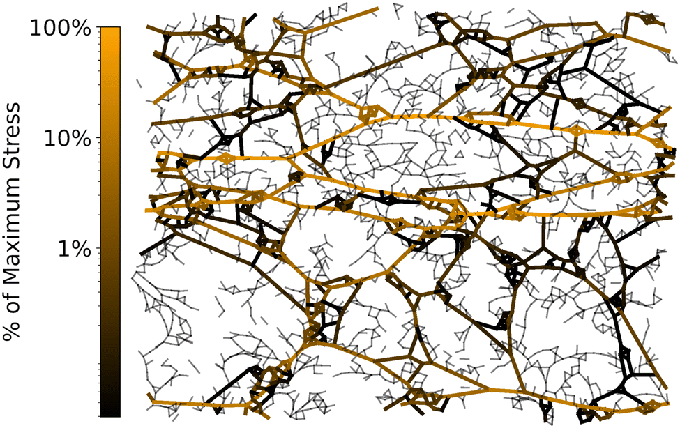
Fig. 1 Rigidity percolation phase diagram and rigid clusters. The location of the phase boundaries are found in the thermodynamic limit using a finite-size scaling analysis. The insets show an anisotropic network close to its rigidity percolation point for the C_xxxx modulus (left) and C_ijkl ≠ C_xxxx moduli (right). The shading corresponds to the energy contributed by each bond after a strain in the x direction (gray indicating little to no stress and brighter indicating higher stress).

2 Methods

2.1 Model for anisotropic rigidity percolation

We generate triangular lattices (coordination number z = 6) of L² sites and periodic boundary conditions in both directions. Bonds are diluted based on their orientation, where p denotes the fraction of occupied bonds in the network. Anisotropy is introduced during lattice generation by filling bonds preferentially based on their orientation. We define the ratio r as the probability of bond occupation along the horizontal direction divided by the probability of bond occupation in the other two independent directions. We then build lattices using methods similar to those previously developed (see Appendix A for details) and investigate the regime where r ≥ 1. Importantly, we are able to adjust r without changing p, which allows us to shuffle bonds and investigate how long-wavelength anisotropy affects the scaling of moduli in equally dense networks. In these coordinates, r = 1 represents a completely randomly diluted triangular lattice and r = ∞ a lattice which has bonds only in the horizontal direction. Our choice of anisotropy for generic r results in four independent long-wavelength components of the elasticity tensor, {C_xxxx, C_yyyy, C_xyxy, C_xxyy}, each of which can be extracted for the various lattices.

2.2 Simulation details

We measure the components of the elasticity tensor for each random lattice realization at different values of filling fraction p, anisotropy r, and linear system size L. To measure these components, we first apply a small external strain ε_ij of magnitude 10⁻³ to ensure we probe the linear response. In the regime of linear elasticity, the energetic cost of such a deformation is quadratic in the strain:

We apply strains ε_xx, ε_yy, and ε_xy to measure the elastic coefficients C_xxxx, C_yyyy, and C_xyxy directly. To measure C_xxyy, we perform a bulk compression and subtract out the energetic contributions from the independently measured C_xxxx and C_yyyy moduli. We introduce strains to the lattice by applying the proper transformation matrix to the positions of each of the nodes. For example, to stretch the network in the horizontal direction (to apply strain ε_xx), the following matrix is applied:

where we set γ to 10⁻³. Since we implement periodic boundary conditions in both directions, all nodes are transformed in the same manner.

In order to measure the energetic costs of our imposed strains in the disordered lattices, we minimize the central-force energy functional over the positions of the nodes. To capture the linear response, we truncate to leading order in the displacement of vertices:

where u_ij is the difference between the displacement vectors for vertices i and j, and r̂_ij is defined as the unit vector between vertices i and j in the initial configuration. The spring constant k_ij connecting sites i and j is either 0 or 1, according to the random number seed, p, and r. For each type of imposed fixed-amplitude strain, we minimize eqn (3) and use the resulting energy and eqn (1) to extract the values of the independent moduli. To improve convergence rates, a Cholesky factorization is computed¹⁶ and used as a preconditioner for a conjugate gradient method¹⁷ (see Appendix B for details). It is worth noting that eqn (3) is valid only in the regime of linear response, which may be violated at higher strains. We verify that our choice of strain, 10⁻³, is sufficiently small by computing the full untruncated energy for a network size of 50 × 50 with p = 0.645 and r = 1.5. These parameters place this network near both rigidity transitions (see Fig. 1) and therefore this network would be most strongly expected to violate linear response. We find that this lattice obeys linear response, with an energy scaling quadratically in strain, up to strains of 10⁻². This indicates that nonlinearities in strain are negligible and eqn (3) is valid in the parameter space we explore here.

We then individually perform scaling analyses for each independent component of the elasticity tensor. Starting with a rigid network, we repeatedly remove bonds and minimize the energy for each strain until the network becomes sufficiently “floppy” in all directions; here, a network is considered floppy in a particular direction if the corresponding modulus falls below a threshold of G_min ≡ 10⁻⁸, which is the simulation tolerance. The moduli as a function of p were averaged for each system size and orientation strength pair (L,r), sampled over 10²–10⁴ random seeds. This procedure allows us to perform a scaling analysis of each component of the elasticity tensor separately.

3 Results

3.1 Isotropic networks

We begin by focusing on the long-wavelength isotropic case, where bonds are removed without regard to their orientation (r = 1). We determine the value of p where each lattice becomes able to support a stress, defined to be p_c. To extrapolate our results to infinite lattices, we conduct a finite-size scaling analysis (Appendix C). For a given system size, we find the rigidity threshold for many different lattices and create a histogram of these p_c values. We find that for increasing lattice sizes, L, the width of the histogram for the threshold values p_c decreases as L^−1/ν. We also find that the mean value of the histogram, 〈p_c〉_L, approaches a value p^∞_c, the threshold in the infinite system, with the same power law:

〈p_c〉_L − p^∞_c ∼ L^−1/ν. (4)

Our analysis determines that p^∞_c = 0.645 ± 0.002, depicted by the black dot along the horizontal axis of Fig. 1, and ν = 1.3 ± 0.2. The location of the threshold at p^∞_c indicates a small deviation from the naïve Maxwell constraint counting, which states that the 2D triangular lattice to have 2 constraints per site, p = 2/3 of the lattice must be occupied. The deviation from this prediction in our measured value of p^∞_c is similar to what is found in other works.⁶ Importantly, we find that in the isotropic system (r = 1) all the moduli share the same threshold value p^∞_c.

Next, we perform a finite-size scaling analysis of each component of the elasticity tensor, which admits a scaling

where δp ≡ p − p^∞_c. Thus, in principle each modulus component could have a different scaling exponent, f^iso_ijkl, and shape, . The universal function is plotted along with the appropriately rescaled data for C_xxxx in Fig. 2. We find excellent scaling for the different system sizes. In the inset of Fig. 2, we plot the collapsed data against the equivalent scaling variable |X|^−ν, which is a more common choice of variables in the literature, but leads to two branches of the scaling function. We find similarly excellent collapses for all the modulus data (see Fig. 9 for the collapse of other components of the elasticity tensor). For all of these analyses we use the threshold p^∞_c = 0.646, the critical exponent ν = 1.3, and obtain f^iso_ijkl = f^iso = 2.2 ± 0.3. Thus, every independent component of the linear elasticity tensor appears to vanish as |δp|^fiso (see Appendix D).

Fig. 2 Universal scaling function for the C_xxxx component of the elasticity tensor at isotropy (r = 1). All data for this component of the elasticity tensor collapse onto a single curve when plotted against the finite-size scaling variable X ≡ (δp)L^1/ν. The inset shows the same collapse against the scaling variable (|δp|^νL)⁻¹ (on a log–log scale). See Appendix D for a similar analysis of the other components of the elasticity tensor. We use p^∞_c = 0.646, ν = 1.3, and f^iso = 2.2 to obtain excellent collapse for all the components of the elasticity tensor.

3.2 Anisotropic networks

We extend our analysis in the previous section to lattices with long-wavelength anisotropy (r > 1), where we preferentially fill bonds in the x direction. We begin with the determination of the phase boundary. For each value of r, we perform a finite-size scaling analysis similar to the one we conducted for the isotropic case: we create histograms of the values of p where C_ijkl vanishes, p^ijkl_c(r), and determine how their mean values extrapolate to the infinite system. For each value of r we find that the mean location of the critical point is well described by:

〈p^ijkl_c(r)〉_L − p^∞,ijkl_c(r) ∼ L^−1/ν′ (6)

Remarkably, we find that for r > 1, the transition for the C_xxxx modulus is distinct from the threshold values for the other components of the elasticity tensor. We find that the phase boundary for C_xxxx bends towards lower values of p with increasing r (Fig. 1). The transition curves for the other moduli appear nearly identical for each system size and bend towards higher values of p with increasing r. This separation indicates a region for which the network is only rigid when strained along the preferred bond orientation direction. We verify these phase boundaries are the same at isotropy but distinct for r > 1 by measuring the separations between the histograms of p_c values for different components of the elasticity tensor as a function of system size (see Appendix E). Thus, the transition from a floppy to a rigid phase occurs in two stages when the system is anisotropic.

We note that for finite system sizes, C_ijkl never truly vanishes on average because if there are enough bonds remaining to create a rigid system-spanning truss , this configuration occurs with finite probability. However, we still expect that in the intermediate regime between 〈p^xxxx_c(r)〉_L and 〈p^ijkl_c(r)〉_L, finite systems will have an elasticity tensor with a principal axis in the x-direction due to our formulation of anisotropy.

Next, we test the scaling behavior of the elasticity tensor components near the critical points. In principle, including anisotropy could introduce corrections to scaling that bend the phase boundary in a trivial way, leaving all critical exponents the same as in the isotropic system. We tested this scenario, by fixing r > 1 and attempting to collapse the data near the relevant p_c(r) values for each component of the elasticity tensor, keeping f^aniso = f^iso and ν′ = ν, but found very poor collapse. This poor collapse suggests that the anisotropic phase transition is in an entirely different universality class, with different values for the critical exponents. We thus conjecture that the vicinity of r = 1 should be analyzed as a crossover scaling between two distinct critical points.

Inspired by renormalization group approaches, we analyze our data using crossover scaling functions expected to be valid in the vicinity of the isotropic critical point:

with r_c ≡ 1. Note that is equal to the previously defined in eqn (5). Based on the form of this crossover scaling function, we expect that the moduli depend upon the anisotropy r only through a second scaling variable, Y; that is, we expect a scaling collapse of all of our data when plotted against X and Y with a single undetermined exponent ζ > 0.

We first estimate ζ by examining the shape of the phase boundaries in the infinite system away from isotropy. Specifically, as shown in Appendix F, because the arguments of the universal scaling function are invariant scaling combinations, this phase boundary must occur at a fixed value of X/Y^1/ζ = δp/(r − r_c)^1/ζ (with corrections to scaling), so that the separation between the two phase boundaries in Fig. 1 scales as (r − r_c)^1/ζ. From this estimate based on the shape of the phase boundaries, we find ζ = 0.25 ± 0.1.

Fig. 3 Crossover scaling of anisotropic rigidity percolation. Each independent elastic modulus, a function of the variables (p,r,L), collapses onto a two dimensional sheet when plotted against scaling variables X ≡ (δp)L^1/ν and Y ≡ (r − r_c)L^ζ/ν. (left) The scaling function and (right) the scaling function . The isotropic data (Y = 0, Fig. 2) is scattered in black, and constant values of Y = 0.66 and Y = 1.65 are scattered in gray (Fig. 15–18). The height contours are projected onto the X–Y plane.

Many other quantities share this crossover scaling ansatz and allow for independent estimates of ζ. The widths of the histograms of p_c values as we tune away from isotropy are also amenable to a crossover scaling analysis, with the variable Y collapsing these widths (Appendix F). From this scaling collapse, we similarly estimate ζ = 0.25 ± 0.1 and find nice collapse (Fig. 13).

This estimate for ζ and the scaling ansatz in eqn (7) can be used to collapse the elasticity tensor components for 250 000 simulations consisting of anisotropy values ranging between 1.0 ≤ r ≤ 2.0, bond occupation values ranging between 0.6 ≤ p ≤ 0.68, and system sizes L ranging between 30 ≤ L ≤ 500. We show a two variable scaling collapse for the C_xxxx and C_yyyy moduli in Fig. 3. We find excellent collapse of each independent modulus onto a two dimensional sheet. The overlaid data points consist of a portion of the data used to produce the sheet and indicate various slices of constant Y: Y = 0, Y = 0.66, and Y = 1.65. The Y = 0 curve (black) shows the finite-size scaling for isotropic systems and is identical to that shown in Fig. 2. We observe similarly excellent collapse at the two higher values of Y (Fig. 15 and 16). For ease of visualization, we also include height contours projected onto the X–Y plane. The height contours for C_xxxx curve toward lower values of X as the scaling variable Y increases, reflecting the fact that the corresponding phase transition curves toward lower values of p as r increases. The other moduli, such as C_yyyy, show the opposite systematic behavior, tending towards higher values of X for increasing Y.

Fig. 4 Generic, isotropic triangular lattice strained in the horizontal direction until it becomes rigid, forming straight lines of bonds important for rigidity. The bonds are shaded corresponding to the energy contributed. Preliminary results suggest that one of the four tangent moduli (C_xyxy) remains zero for a range of strains above the strain stiffening threshold, with C_xxxx being the dominant modulus.

The critical exponents determined thus far, including ζ, are properties of the isotropic rigidity percolation critical point. We are also interested in the anisotropic critical exponents, such as the critical exponent with which each modulus vanishes with p in an infinite anisotropic system (f^aniso_ijkl). The universal scaling function for the crossover between the isotropic and anisotropic critical points in principle contains all of these anisotropic critical exponents in its singularities in various asymptotic regimes. However, it is quite difficult to get reliable high-precision fits to generic two-variable scaling functions that include precise information about their singularities. We instead independently estimate f^aniso_ijkl by examining the largest system sizes of simulations performed at r = 1.2, 1.5. In addition, we analyze the data for Y = 0.66, 1.65.

We find that the critical exponents for C_xxxx are distinct from those found for the isotropic system while those for the other elasticity tensor components cannot be distinguished from those found for the isotropic system:

with f^aniso_xxxx = 4.0 ± 1.0, compared to our estimate of f^iso = 2.2 ± 0.3. As usual in crossover scaling, the multicritical point governs short length scales and regions far from the critical lines emanating from it. We thus expect to find a crossover from f^aniso_xxxx to f^iso_xxxx as networks move away from the anisotropic critical point, as demonstrated in Fig. 14. We also attempt to independently estimate ν^aniso, the finite-size scaling exponent away from isotropy, using the collapse plots shown in Fig. 13 (Appendix F), but our estimates span a wide range of values 1.2–3.2. Our estimates for all scaling exponents are shown in Table 1.

Table 1 Numerical estimates of critical exponents

Exponent	Estimate
ν	1.3 ± 0.2
f ^iso	2.2 ± 0.3
ζ	0.25 ± 0.1
ν ^aniso	1.2–3.2
f ^aniso xxxx	4.0 ± 1.0
f ^aniso ijkl (ijkl ≠ xxxx)	2.2 ± 1.0

---

4 Conclusions

We find that rigidity percolation in our model anisotropic system occurs in at least two steps, with the modulus in the direction of alignment becoming nonzero at lower volume fractions. Our estimate of at least one of the critical exponents of the anisotropic transition, f^aniso_xxxx, appears distinct from the corresponding exponent for the isotropic transition f^iso, which suggests that these anisotropically diluted networks feature two distinct universality classes.

It was a surprise to us that the rigidity percolation transition for the isotropic lattice broke up into several transitions when it became anisotropic. First, obtaining multiple transitions is contrary to the naïve usage of Maxwell counting to determine the location of the rigidity transition. As shown in the insets of Fig. 1, the rigid modes become anisotropic, and span horizontally before they span vertically.

Second, our results are fundamentally different from connectivity percolation, where regardless of the value of r there can only be one transition. The left inset in Fig. 1 shows several horizontal stress-supporting chains spanning the network. The critical point at which C_xxxx first becomes non-zero presumably separates a phase where there are no stress-supporting chains from one where there are a finite density of such chains. In regular percolation, two such paths connecting the system horizontally that are separated by any finite distance will have a finite probability per unit length of being connected by bonds extending in the vertical direction. Hence, for ordinary percolation, as soon as one crosses the horizontal percolation point in an anisotropic system, it must percolate in the other directions as well. This argument suggests that lattices with bending stiffnesses and angular springs, which are believed to become rigid at the connectivity percolation threshold,⁵ lack this intermediate phase. However, in typical situations where bending stiffnesses are much weaker than stretching stiffnesses, a remnant of this intermediate phase should be measurable even when bending is included.

In retrospect, we should have expected separate transitions in central force rigidity percolation on regular lattices. Maxwell counting tells us when the number of zero modes can vanish in the absence of states of self stress, but does not tell us whether the zero modes couple to a given mode of deformation.^18,19 Straight lines of bonds supporting stress in a large system, when connected vertically, may only contain contributions to the stress that grow quadratically (i.e. non-linearly) in the strain: the length of a beam connecting (x,y) to (x′,y + ε) grows as ε², suggesting the corresponding linear elastic modulus is 0. A similar nonlinear response to infinitesimal strains is found to stabilize hypostatic jammed packings of ellipsoidal particles,²⁰ in violation of simple constraint-counting arguments. The perfect square lattice has no C_xyxy shear modulus, and the perfect hexagonal lattice has no non-zero moduli except the bulk modulus – why should anisotropic random lattices not possess separate transitions?

Since generic lattices have no straight lines of bonds, it is not clear to us whether they will have intermediate phases with infinite anisotropy in linear response. (Indeed, a non-generic lattice which supports horizontal strain under tension has straight lines of bonds that buckle under compression making the effective modulus under compression still zero). Even in this case, we expect crossover scaling to be an important component of the analysis of anisotropic generic lattice networks. Our analysis suggests that the scaling of anisotropic generic networks could exhibit a crossover between distinct rigidity transition universality classes.

The difference between generic and non-generic lattices is no longer crucial after finite deformations; under tension a node connecting only two bonds will naturally straighten out to 180° and not support perpendicular stresses to linear order. Along these lines it might be interesting to investigate whether separate rigidity transitions arise in floppy isotropic random lattices under finite deformation. Preliminary results suggest strain stiffening leads to rigidity along the extension axis without rigidity under some of the other modes of deformation (see Fig. 4).

What kind of rigidity critical points do we expect? The C_xxxx transition where horizontal stress-bearing chains first arise could be self-similar (with a single diverging correlation length), but could also be self-affine (with the vertical spacing between chains diverging with a different power on the stress-supporting side than the rigid cluster lengths diverge on the floppy side, akin to directed percolation, where connectedness lengths are controlled by different critical exponents parallel and perpendicular to the preferred direction^21–23). Whether the three other moduli become non-zero simultaneously or separately in this model is not numerically resolved yet, but one expects that more complicated anisotropies (say a 3D model with brick-like symmetry) will allow for separate transitions for those moduli as well.

Finally, it would be interesting to consider whether the results presented here have any bearing on biological networks. Many biological tissues, including bone, tendon, muscle, and blood vessels, have an extracellular matrix that exhibits preferential alignment, giving rise to anisotropic elastic moduli. It may be possible to understand the extracellular matrices of these tissues as anisotropic networks which have crossed the rigidity percolation transition in the stiff direction, but not the other directions. A quantitative description of these tissues may require analyzing the effects of second-order constraints, changing the contact number distribution, and exploring the crossover between this pair of zero-bending stiffness transitions and a bending-dominated regime. Moreover, cells are able to control how matrix elements are generated. Cells may generate networks with many different rigidity transitions to tune between, where the particular way matrix elements are laid down biases the thresholds of the different components of the elasticity tensor. As such, the results presented here could have profound implications for understanding more complicated networks in many biological systems.

Data availability

The data used in this study are available at doi.org/10.5281/zenodo.13910625. The code for the network simulations can be found at doi.org/10.5281/zenodo.13894006.

Conflicts of interest

There are no conflicts to declare.

Appendices

A: Bond filling protocol

One method for filling the lattice is to choose some number of bonds n to randomly occupy, and set p = n/N, where N is the total number of possible bonds. This has the disadvantage that changes in p can only be measured to a sensitivity 1/N. To characterize the behavior very close to the critical point, we instead fill our lattice in a way that is statistically equivalent, but allows measurements at continuous values of p. In the isotropic case, the algorithm is as follows: first, a random number s_i taken uniformly between 0 and 1 is assigned to each bond i. At a filling parameter value p, all bonds i with assigned random numbers s_i < p are filled, and the independent components of the linear elasticity tensor are measured through applied shears. For different random number seeds, the “jumps” in the linear moduli associated with the addition of single stress-supporting bonds to the rigid backbone occur at different values of p (which are not multiples of 1/N). When the measurements are averaged over several random number seeds, we find that the measurements of moduli quickly converge to a smooth function of p at a given system size L, except at the smallest values of p. This algorithm is modified to include our anisotropy parameter r in a straightforward way.

We start by picking a random number seed, and then assigning a (uniformly chosen) random number s_i between 0 and 1 to each bond. The bonds are assigned and then sorted based on a key, k_i, which corresponds to the value of bond occupation fraction p for which the bond would be added based on the anisotropy parameter r:

where s^x_i are assigned to bonds in the horizontal direction and s^y_i are assigned to the other bonds. The bonds are then removed according to their keys, highest to lowest. Note that this formulation allows for finding the bond configuration while continuously varying both p and r.

B: Numerical methods

We minimize the energy given in eqn (1), which can be equivalently written aswhere H is the Hessian matrix and u⃑ is a length N × d vector containing the displacements from the initial node position.

To handle periodic boundary conditions, we split the Hessian into two parts: H_pbc, which is computed using only the bonds that span across the network, and H_in with bonds which do not. The energy is therefore computed as:

in which c⃑ “corrects” the displacements for nodes that are connected across the network and depends on the particular strain. The energy is then minimized by finding a zero-force configuration, solving the following linear system:

(H_in + H_pbc)u⃑_relaxed = −H_pbcc⃑ (12)

An affine displacement is used as an initial guess. The sparsity structure allows matrices to be stored in compressed sparse row format, reducing memory usage and improving the speed of operations. A Cholesky factorization for (H_in + H_pbc) is computed¹⁶ and used as a preconditioner. For large system sizes, we use GPUs to accelerate numerical computations, such as matrix factorizations and matrix-vector products.

We note that for systems that have under-constrained nodes, the null space of (H_in + H_pbc) has a non-zero dimension; as such we do not consider the non-affinity parameter (which sums the squared displacements from an affine transformation) as a method of analysis or for extracting critical exponents.

C: Details of finite-size effects

To obtain a consistent estimate of p^∞_c and ν, we consider the distribution of the rigidity percolation threshold for each modulus at isotropy (r = 1). We take p^ijkl_c to be the smallest value of p at which C_ijkl is rigid. For a given system size L, the value of p^ijkl_c is sampled from an underlying distribution:

p^ijkl_c(L) ∼ ρ^ijkl_L, ρ^ijkl_L ∈ Δ[0,1]. (13)

Histograms of p^ijkl_c are plotted in Fig. 5. As the system size increases, the distributions become increasingly sharp and the means shift systematically. In the limit of infinite system size, we assume that each distribution converges to a delta function about p^∞_c.

Fig. 5 Histograms of rigidity percolation threshold p_c as a function of system size L at isotropy. The estimated density functions for each independent elastic modulus are plotted. Each distribution becomes increasingly sharp with larger system size.

For each system size, we compute both the means 〈p^ijkl_c〉_L and standard deviations σ^ijkl_L of each distribution. We expect systematic shifts in the means and standard deviations (i.e., the first and second moments) to scale as a power law with respect to L governed by a single critical exponent ν:

We perform a joint non-linear least squares fit,²⁴ with p^∞_c and ν the same for all curves (we assume they are equal for each modulus at isotropy). Fig. 6 depicts 〈p^ijkl_c〉_L (left) and σ^ijkl_L (right) as a function of L. The fits give an estimate of p^∞_c = 0.645 ± 0.002 and ν = 1.3 ± 0.2.

Fig. 6 (left) Mean of p_c and (right) standard deviations of the p_c distribution at isotropy as a function of system size. The fitted curves match those in eqn (14) and the fitted lines on the right figure have slope −1/ν.

Furthermore, we find a universal scaling function for the distributions ρ^ijkl_L with respect to our previously defined scaling variable X ≡ (δp)L^1/ν:

We find that X collapses the density functions, with the resulting histograms shown in Fig. 7.

Fig. 7 Universal scaling of rigidity distributions at isotropy for each independent modulus. The histograms all collapse when plotted against the scaling variable X.

D: Details of modulus scaling collapse

At isotropy, each modulus grows as a power law above rigidity percolation threshold C_ijkl ∼ (δp)^fiso. Fig. 8 depicts the uncollapsed finite-size scaling data at isotropy; the systematic deviations are clear.

Fig. 8 Unscaled modulus data across various system sizes at isotropy (r = 1). The smaller system sizes have a higher probability of becoming rigid at lower values of p.

We find the exponent f^iso by considering the largest available system size (L = 500) and performing a least-squares fit of the modulus, finding a range of f^iso as we vary p_c slightly. With f^iso = 2.2, p^∞_c = 0.646, and ν = 1.3, we plot the data against the proposed scaling variables and find a nice collapse for all independent moduli, shown in Fig. 9. The number of samples we average over ranges from 10⁴–10² for system sizes L ∈ [30,200] and 20 samples of L = 500.

Fig. 9 Universal scaling function of all independent elastic moduli at isotropy (r = 1). The independent components of the elasticity tensor each collapse onto a single curve when plotted against the finite-size scaling variable X ≡ (δp)L^1/ν. In this isotropic case, there are only two independent moduli in the long-wavelength elasticity tensor (B and G, for instance).

Using the value of f^iso = 1.4 ± 0.1 and ν = 1.4 ± 0.2 quoted in Broedersz et al.,⁶ we find best collapse with p^∞_c = 0.65 shown in Fig. 10, which gives good collapse for lower values of system size, but does not collapse the modulus for our largest system.

Fig. 10 Universal scaling function of all independent elastic modulus using previously reported exponents.⁶ The data for the range L ∈ [30,200] comparable to the earlier work does give a good collapse. Having the larger system size (L = 500) explains why we find different exponents.

E: Separation of phase transitions

Here we present our numerical evidence for the separation of the two phase transitions (one for C_xxxx, and at least one additional for C_ijkl with ijkl ≠ xxxx) as L → ∞. We do this by analyzing the systematic dependence on L of the distributions of p_c for each modulus away from isotropy, i.e., we perform large numbers of simulations at various system sizes for fixed r = 1.5 (away from isotropy) and examine how these distributions depend upon L. An example of these distributions can be seen in Fig. 11, where at L = 75 (first column) the distributions of p_c for the C_xxxx and the C_yyyy moduli have significant overlap, but when we look at L = 200 (second column) the distributions are beginning to separate for r > 1.

Fig. 11 Histograms of rigidity percolation threshold p_c for C_xxxx (blue) and C_yyyy (green) for the same system size. The means are consistent at isotropy (r = 1) and distinct from each other at higher anisotropy (r = 1.5).

Sample-to-sample, there are lattices that can support rigidity in some shear directions but not others. There are two basic scenarios. (1) In the case where including anisotropy ends up simply giving analytic corrections to scaling that bend a single phase boundary, all moduli will vanish at the same location at L = ∞, but the amplitudes of the finite-size effects may be different. Singling out the C_yyyy modulus for the sake of comparison, this means that

〈p^ijkl_c〉_L − 〈p^yyyy_c〉_L ∼ L^−1/ν. (16)

This is the same as the asymptotic scaling for the spreads of these distributions, σ^ijkl_L ∼ L^−1/ν, as all distributions are controlled by the exponents of the isotropic critical point in this supposition. If we measure the separation between the means as a function of system size in terms of the number of standard deviations of the distribution at that system size, using the more democratic σ_L² = (σ^ijkl_L)² + (σ^yyyy_L)², then, we should findfor some constant c_ijkl, which is flat as a function of system size.

(2) In the case where including anisotropy leads to genuinely new critical phenomena and a pair of phase transitions, the finite-size effects of the mean and standard deviation are controlled by the finite-size scaling exponent of each anisotropic rigidity transition ν^aniso. If we split into a pair of phase transitions, then the spreads σ_ijkl of each distribution will narrow with increasing L, but the separation of the means is asymptotically constant as L → ∞. This would make

where ν^aniso is the largest of the (potentially different) finite-size scaling exponents associated with the new, anisotropic transition.

We begin by performing this measurement of the separations between the distributions of p_c for all moduli at the isotropic transition, where all moduli vanish at the same location in p as L → ∞ (Fig. 12 (left)).

Fig. 12 Separation of rigidity percolation threshold mean 〈p_c〉 from that of the C_yyyy modulus as a function of system size at isotropy (left) and anisotropy (right).

As expected, this measure of the separation in the means is flat for the isotropic case as a function of system size, confirming that these moduli vanish at the same asymptotic location and that the finite-size effects controlling the mean and the standard deviation have the same systematic dependence on L.

When we perform the same analysis for the anisotropic case (r = 1.5), we see systematic growth in this measure as a function of system size (Fig. 12 (right, blue)), suggesting that the locations of p_c for different moduli are genuinely different in the thermodynamic limit. This is moderately strong quantitative evidence for the information that can roughly be seen by eye in Fig. 11.

F: Estimate of anisotropic scaling exponents

At infinite system size, the phase diagram curves in Fig. 1 contain important information about the critical exponent ζ near the isotropic transition. We find ζ by fitting the differences between the C_xxxx curves and the C_ijkl curves (where ijkl ≠ xxxx) to a power law, resulting in a value of ζ = 0.25 ± 0.1. The individual phase boundaries have an important linear correction to scaling, as the unstable eigenvector is not along the r-axis, but has a slope m. Hence the two phase boundaries are of the form δp = m(r − r_c) + W(r − r_c)^1/ζ, with a fixed value of W defining a curve along which the invariant scaling combination is constant. Because ζ is small, this correction cannot be neglected. By fitting the differences between the phase boundaries, we bypass this linear correction to scaling.

Furthermore, we can consider the standard deviations of the rigidity percolation threshold distributions (as in Appendix C) for r > 1 and consider a scaling function with respect to our scaling variable Y = (r − 1)L^ζ/ν

We find that standard deviation is best collapsed with ζ = 0.25 ± 0.1, shown in Fig. 13. The determined value of the exponent ζ appears to collapse σL^1/ν for all moduli except for C_xxxx at larger values of the scaling variable. We also note the nice overlap of data performed at different values of (r,L) but the same value of the scaling variable Y.

Fig. 13 Universal scaling of rigidity distributions near isotropy for each independent modulus. The widths of the histograms all collapse onto a single curve when plotted against the finite-size scaling variable Y. There appear to be deviations in the collapse of the C_xxxx modulus at higher values of Y.

Fig. 14 Estimate of anisotropic scaling exponent of each modulus from our largest system size. The behavior of the C_xxxx modulus suggests a crossover between the anisotropic and isotropic scaling exponents, whereas for the other moduli, the behavior appears to be governed by the same isotropic exponent.

We can in principle use information from these collapse plots to make a prediction for the value of the finite-size scaling exponent close to the anisotropic phase transition ν^aniso. First, we note that if we fix r > 1 and send L → ∞, the spread in the distributions of p_c will narrow as σ ∼ L^−1/νaniso, as the finite-size effects are (at large enough system sizes) controlled by the critical exponents of the anisotropic critical point. In the scaling function for the distributional spreads of p_c, this corresponds to the asymptotic limit Y → ∞. Forcing the asymptotics of the numerically determined crossover scaling function to agree with the asymptotics expected at the anisotropic critical point will give us a prediction for ν^aniso.

Suppose this scaling function has asymptotic behavior at large Y. Then in the limit L → ∞ with r > 1 fixed,

σL^1/ν ∼ Y^α ∼ L^ζα/ν and σ ∼ L^−1/νaniso (20)

together givewhere ν is the value of the finite-size scaling exponent at the isotropic fixed point. With α = 1.0 ± 0.5, this gives a prediction of ν^aniso = 1.7, but values between 1.2–3.2 are consistent with our error bars reported in Table 1. This is ultimately due to the poor numerical determination of ζ and α. These could also in principle be different for the different ijkl; this would be detected through different values of α for each modulus since both ν and ζ are properties of the isotropic fixed point.

We estimate the exponent with which each modulus vanishes at their corresponding anisotropic phase transition (f^aniso_ijkl) by considering our largest system size at two values of r away from isotropy (r = 1.2 and r = 1.5). The location of the phase transition is determined by averaging the value of p with which each modulus for each lattice becomes rigid.

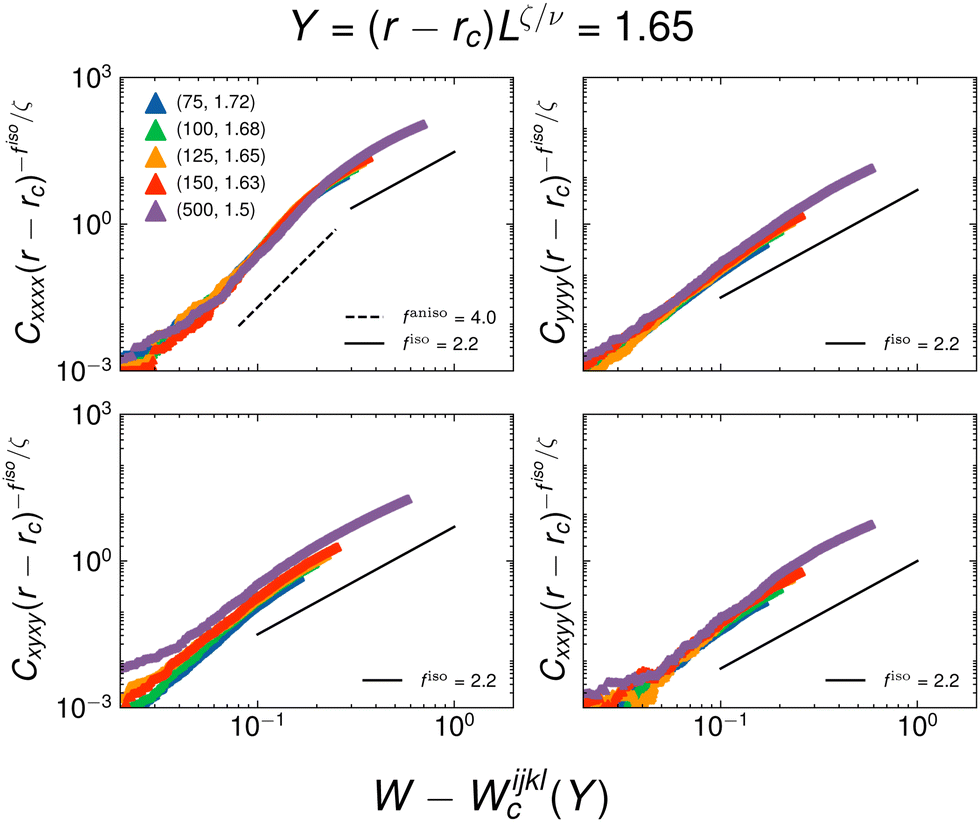
To search for which value of ζ best collapses the two variable scaling function, we obtain simulations of constant Y across various system sizes. We test a value of ζ by first fixing our largest system size and then solving for the value of r as a function of system size that results in the same value of Y. Fig. 15 and 16 show a scaling collapse of all the moduli with ζ = 0.25 and with a constant value of Y = 0.66 and Y = 1.65, respectively. The scaling function for each modulus vanishes at a given value of W, which we denote as W^ijkl_c(Y), as it is dependent on the value of Y. We note that further away from isotropy (Y = 0), there are additional corrections to scaling, resulting in a worse collapse at higher values of Y.

Fig. 15 Scaling collapse of all the moduli at constant Y = 0.66. The estimate of W_c is shown with the dashed black line.

Fig. 16 Scaling collapse of all the moduli at a constant Y = 1.65. The estimate of W_c is shown with the dashed black line.

We again obtain an estimate of the scaling exponents in Fig. 17 and 18 by plotting the rescaled moduli as a function of distance from W_c. The plots suggest crossover for the C_xxxx modulus, with f^aniso_xxxx governing the behavior for lower values of W − W_c and f^iso for the high W − W_c regime. Furthermore, the other three moduli appear to vanish with a critical exponent indistinguishable from f^iso within our estimated error bars.

Fig. 17 Estimate of anisotropic scaling exponent of each modulus at a constant Y = 0.66. The simulation data is the same as found in Fig. 15.

Fig. 18 Estimate of anisotropic scaling exponent of each modulus at a constant Y = 1.65. The simulation data is the same as found in Fig. 16.

Acknowledgements

The authors acknowledge Thomas Wyse Jackson for critical discussions in the early phases of the project. WYW, IC, NS, SJT, and JPS are supported by NSF DMR 2327094. JO was supported in part by the NSF MRSEC DMR-1719875. BC was supported by NSF CBET award number 2228681 and NSF DMR award number 2026834. AB is supported by NSF DGE 2139899. JAM and MD are supported by NSF EF 1935277.

Notes and references

1. S. Thomopoulos, J. P. Marquez, B. Weinberger, V. Birman and G. M. Genin, J. Biomech., 2006, 39, 1842–1851.
2. T. Zhang, J. M. Schwarz and M. Das, Phys. Rev. E:Stat., Nonlinear, Soft Matter Phys., 2014, 90, 062139.
3. T. Wyse Jackson, J. Michel, P. Lwin, L. A. Fortier, M. Das, L. J. Bonassar and I. Cohen, Sci. Adv., 2022, 8, eabk2805.
4. J. L. Silverberg, A. R. Barrett, M. Das, P. B. Petersen, L. J. Bonassar and I. Cohen, Biophys. J., 2014, 107, 1721–1730.
5. M. Das, D. A. Quint and J. M. Schwarz, PLoS One, 2012, 7, 1–11.
6. C. P. Broedersz, X. Mao, T. C. Lubensky and F. C. MacKintosh, Nat. Phys., 2011, 7, 983–988.
7. D. J. Jacobs and M. F. Thorpe, Phys. Rev. E:Stat. Phys., Plasmas, Fluids, Relat. Interdiscip. Top., 1996, 53, 3682–3693.
8. S. Feng and P. N. Sen, Phys. Rev. Lett., 1984, 52, 216–219.
9. J. Currey, K. Brear and P. Zioupos, J. Biomech., 1994, 27, 885–897.
10. S. Weiner and H. D. Wagner, Annu. Rev. Mater. Res., 1998, 28, 271–298.
11. B. Hoffmeister, S. Handley, S. Wickline and J. Miller, J. Acoust. Soc. Am., 1996, 100(6), 3933–3940.
12. A. de Aro, B. de Campos Vidal and E. Pimentel, Micron, 2012, 43, 205–214.
13. S. Zhang, L. Zhang, M. Bouzid, D. Z. Rocklin, E. Del Gado and X. Mao, Phys. Rev. Lett., 2019, 123, 058001.
14. J. Michel, G. von Kessel, T. W. Jackson, L. J. Bonassar, I. Cohen and M. Das, Phys. Rev. Res., 2022, 4, 043152.
15. A. Sharma, A. J. Licup, K. A. Jansen, R. Rens, M. Sheinman, G. H. Koenderink and F. MacKintosh, Nat. Phys., 2016, 12, 584–587.
16. Y. Chen, T. A. Davis, W. W. Hager and S. Rajamanickam, ACM Trans. Math. Software, 2008, 35, 22.
17. J. Nocedal and S. J. Wright, Numerical Optimization, Springer, 2nd edn, 2006, ch. 5, pp. 101–134.
18. O. K. Damavandi, V. F. Hagh, C. D. Santangelo and M. L. Manning, Phys. Rev. E, 2022, 105, 025003.
19. O. K. Damavandi, V. F. Hagh, C. D. Santangelo and M. L. Manning, Phys. Rev. E, 2022, 105, 025004.
20. A. Donev, R. Connelly, F. H. Stillinger and S. Torquato, Phys. Rev. E:Stat., Nonlinear, Soft Matter Phys., 2007, 75, 051304.
21. J. Wang, Z. Zhou, Q. Liu, T. Garoni and Y. Deng, Phys. Rev. E:Stat., Nonlinear, Soft Matter Phys., 2013, 88, 042102.
22. I. Jensen, J. Phys. A: Math. Gen., 1999, 32, 5233–5249.
23. A. Hansen and S. Roux, J. Phys. A: Math. Gen., 1987, 20, L873.
24. M. Newville, T. Stensitzki, D. B. Allen and A. Ingargiola, LMFIT: Non-Linear Least-Square Minimization and Curve-Fitting for Python, 2015.

---