Poly(ε-caprolactone-co-ε-decalactone)/carbon black or carbon nanofiber composites. Synthesis, morphological, and thermal/electrical properties

Abstract

Much of the research on biodegradable polymers is currently aimed at developing alternative materials to fossil fuel plastics. Among the biodegradable polymers, the bio-based aliphatic polyesters (e.g. poly-ε-caprolactone, PCL) have had important success in replacing single-use plastics as well as durable consumer goods, mainly in the packaging and biomedical sectors. In other sectors, like electronics, the use of bio-based plastics has received little attention, despite e-waste (pollutant and difficult to handle) being the fastest growing solid waste stream in the world. In this work, P(CL–DL)/carbon black and P(CL–DL)/carbon nanofiber composites with enhanced thermal and electrical properties were prepared and studied. P(CL–DL) copolymers were synthesized via ring opening polymerization (ROP) at CL/DL molar compositions of 95/5, 90/10, 80/20, and 70/30. Their number-average molecular weight (M̄_n) and dispersity index (Đ) lie between 17.5 and 21.8 kDa, and 1.72 and 1.99, respectively. They are thermally stable to up to 300 °C, and show a melting temperature (T_m) and a crystalline degree (X_c) that decrease with increasing contents of DL in the polymer chains. The thermal (k) and electrical (σ) conductivities of copolymers were enhanced by adding, through melt blending, carbon black (CB) or carbon nanofibers (CNF) at 1.25, 2.5, and 5.0 wt%, reaching a maximum value of 0.55 W m⁻¹ K⁻¹ and 10⁻⁷ S cm⁻¹, respectively. The frequency-dependence of the dielectric constant (ε′) and dielectric losses (tan δ) was also measured. Two of the composites showed a marked increase of ε′ near percolation whereas their tan δ remained low. The thermal and electrical conductivity performances, as well as the increment found in ε′ near percolation, are discussed in terms morphology changes produced by variations in both the DL mol% and the nanoparticles wt%. Finally, biodegradable composites with heat and electron dissipative capacities are materials that can contribute to alleviating the problem of e-waste.

---

1. Introduction

In the last decades, the electronics industry has experienced fast growth due to extraordinary advances in e-technology and materials that have permitted the creation of a wide variety of items of practical use in our daily lives. However, the exponential growth in the consumption and disposal of such items has led to a rapid increase of e-waste, with the consequent impact on the environment.¹ It is worth mentioning that polymers or plastics account for 20 to 30 wt% of the total e-waste.² Unfortunately, they are mostly non-biodegradable fossil fuel-based polymers whose complex mix with metals and hazardous components makes their recycling challenging and frequently unaffordable. There is thus a need to develop a sustainable electronics industry, for instance, by including bio-based polymers (pristine or modified) with the appropriate characteristics and properties.^3,4

Aliphatic polyesters synthesized from renewable sources like biomass, organic oils and terpenes, are biodegradable polymers that can be used in electronics.^5,6 Among the variety of aliphatic polyesters, polycaprolactone (PCL) is attracting great attention because it is a long-standing material that fully degrades in 2–4 years at natural soil conditions or in few weeks at specific biodegradation or hydrolytic conditions.^7,8 Its easy processing (e.g. injection molding) and shaping (e.g. 3D printing) allow the fabrication of almost any polymer-based electronic component.^9–11 PCL by itself can be used as a cost-effective flexible substrate for electronic circuitry.¹² It can also be used as a binder in graphene nanoplatelet (GNP) nanopapers to create heat spreaders showing a higher mechanical resistance than those based on neat GNP.^13,14 PCL-based nanocomposites have been developed with specific properties to work as photo-thermal absorbers,¹⁰ temperature-dependent switch materials,¹⁵ electromagnetic interference shielding composites,¹⁶ etc. Other applications may be envisaged for the electro conductive PCL-based nanocomposites taking advantage of its biocompatibility.^17,18

PCL-based nanocomposites with enhanced thermal and/or electrical conductivity capacities have potential use in flexible electronics.^5,14,19 A classical approach to increase the thermal and electrical conductivities of polymeric materials (traditionally insulators) is through the incorporation of small amounts of high conductive nanoparticles, either inorganic, metallic, ceramic, or carbon-based.^20–22 The carbon-based ones like carbon nanotubes (CNT), carbon nanofibers (CNF), and GNP stand out by their own thermal (k) and electrical (σ) conductivities that surpass those of any other conducting nanoparticle.²³ Carbon black (CB) is another carbonaceous particle that has been traditionally used to enhance the electron transport in polymers.^24,25

In the preparation of polymer nanocomposites, homogeneous dispersion and good polymer-particle interaction are critical issues as they determine the final properties and potential applications.²⁶ From the different mixing or dispersing methods (melt processing, solution, in situ, etc.), melt processing (e.g. extrusion) is often preferred. Its performance may not be as good as that of the others, but is cheap, not pollutant, and can afford the required dispersion and inter-particle contacts to create the conduction networks through which electrons move.²¹ The transport of phonons also depends on the content and dispersion of particles,²⁷ although the crystalline degree of samples and the characteristics (resistance, charge trap, etc.) of the polymer-particle interface are critical factors.²⁸ Nanoparticles having a high aspect ratio like CNT, CNF and GNP are able to provide inter-particle contact at low loadings,^27,29 although in economy terms, CNFs are preferred by their low cost, low tendency to self-aggregate, and capacity to confer to polymers the required thermal/electrical conductivity properties.^30,31

PCL and PCL-based copolymers and blends have been selected by some research groups as base polymers to develop thermal and electrical-conducting nanocomposites through different methods and using different types of nanoparticles.^11,22,32 Most reports in this concern involve multiwall carbon nanotubes (MWCNT), which provide high electrical and thermal conductivities at low particle contents (between 0.1 and 2 wt%).^33–35 Good interaction between MWCNT and the matrix allows the formation of homogeneous dispersions. Adding a third component³⁶ or introducing (grafting) polymers on the surface of the MWCNT are two of the various strategies to improve interaction and/or dispersion, although thin polymer films over nanotubes may result in a poor inter-particle contact.³⁷ CNF, GNP, CB, and reduced graphene oxide (r-GO) have also been used in the preparation of conductive PCL-based nanocomposites with satisfactory results.^13,38 Small amounts of a co-monomer like ε-decalactone (DL) can decrease the polymer stiffness while the crystalline structure is partially retained, making thus the P(CL–DL) copolymer suitable as a base polymer for flexible electronics.

In the present study, P(CL–DL)/CNF and P(CL–DL)/CB composites were prepared and their thermal and electrical properties were studied. Results are discussed in terms of morphology and interaction changes produced by variation in DL and nanoparticle contents.

2. Experimental part

2.1 Regents, solvents and nanoparticles

ε-Caprolactone (ε-CL), ε-decalactone (ε-DL), benzyl alcohol (BzOH), trioxane (all four from Sigma-Aldrich, St. Louis, MO USA), 1,5,7-triazabicyclo[4.4.0]dec-5-ene (TBD) (from TCI chemicals, Portland, OR, USA), and methanol (from J. T. Baker, Radnor, PA, USA) were used as received. Toluene (from J. T. Baker, Radnor, PA, USA) was washed with H₂SO₄, neutralized with a NaHCO₃ solution (10 w%), dried with CaCl_2, and distilled using a sodium/benzophenone complex. Conductive grade carbon black XC68 was supplied by Cabot Corporation (Canada). Carbon nanofibers (CNF) HHT grade (PR-24-XT-HHT) were provided by Pyrograf Products, Inc., with an average diameter of 100 nm, length from 50 to 200 μ, and purity of 95%.

2.2 Synthesis of the P(CL–DL) copolymers

Copolymers were prepared at CL–DL contents of 95–5, 90–10, 80–20 and 70–30 mol%. ε-CL, ε-DL and toluene were first introduced in a 1 L batch reactor and the reaction (polymerization) conditions were set to 400 rpm, 100 °C and N₂ atmosphere before adding dropwise a solution of BzOH, trioxane, and TBD in toluene (20 mL), according to data listed in Table 1. Trioxane was used as a NMR standard to monitor the reaction conversion (yields ≥ 80% for all reactions). A 1 L stainless steel batch reactor Delta Reactory (Fig. 1), equipped with mechanical stirring, internal coil cooling system, and electric resistance heating system, was used for polymerizations. Each copolymer was precipitated in 1.5 L of cold methanol (∼0 °C) while stirring the solution at 300 rpm for 1 h. Solutions were filtered and the recuperated white solids (copolymers) were dried overnight in a vacuum oven set at 35 °C and 30 mm Hg. A schematic representation of the polymerization reaction is shown in Fig. 2. The Greek letter ε was omitted in labels of polymers and composites to make them shorter.

Table 1 Molar amounts of chemicals used in the synthesis of polyesters^a

Polyester	ε-CL (mol)	ε-DL (mol)	TBD (mol)	BzOH (mol)	T (h)
a In all cases trioxane (0.05 moles).
PCL	6.0	0	0.05	0.01	5
P(CL95–DL5)	5.7	0.3	0.05	0.01	48
P(CL90–DL10)	5.4	0.6	0.05	0.01	48
P(CL80–DL20)	4.8	1.2	0.05	0.01	72
P(CL70–DL30)	4.2	1.8	0.05	0.01	96

---

Fig. 1 Schematic diagram of the reactor used for polymerization.

Fig. 2 Ring opening polymerization of ε-CL and ε-DL into P(CL–DL) copolymer. Both monomers are randomly distributed in the polymer chain. m and n correspond to the mol% of each monomer in copolymers.

2.3 Preparation of the P(CL–DL)/CB and P(CL–DL)/CNF composites

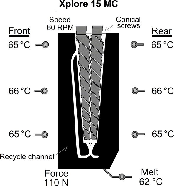
Polyesters and nanoparticles (1.25, 2.5, and 5.0 wt% of CB or CNF) were introduced into a beaker. Polyesters are fine powders, so they were first hand-mixed (spatula) with CB or CNF particles up to observe a homogeneous black colored mixture. The homogeneous mixture was then introduced into an Xplore MC 15 co-rotating twin-screw micro compounder through a hopper, consisting of a funnel, a plunger and a hollow pipe. When the micro compounder was full, the hopper was removed from the Barrel to further attach a seal plug in place. The micro compounder was operated at a screw speed of 60 rpm, a temperature ranging between 50 and 70 °C and a residence time of 10 min. No inert gas (N₂) was supplied during processing because polycaprolactone is thermally stable to up to 260 °C under atmosphere conditions (air), as it was demonstrated by thermogravimetric analysis (ESI, Fig. S1†).

Fig. 3 shows a scheme of the configuration of the twin-screw micro compounder in which the processing conditions for the preparation of one the composites (PCL/CNF_5.0) are displayed. The conical form of screws provides an effective compacting and high pressure at the exit. The six heating zones in the barrel are independently adjustable. The recycle channel allows the mixed materials be pumped around, in such a way that the compounding process can be extended to any desired time. This may correspond to the increase of L/D in a continuous twin-screw extruder. Some features of the micro compounder are: length of screws 172 mm, total volume 16.5 mL, net volume 15 mL, revolutions 5 to 250 rpm, and number of heating zones 6. Easy and fast recuperation of the all composite (no material is lost) as well as easy cleaning are some advantages of the Xplore 15 MC micro compounder. It is noteworthy to mention that this equipment was designed for fast and efficient compounding/mixing of small quantities of material, and therefore its use is convenient for the development of new materials at lab scale.

Fig. 3 Schematic representation of the configuration of the twin-screw micro compounder.

In order to avoid hydrolytic degradation, polyesters were dried during 24 h in a vacuum oven (set at 45 °C) prior to the extrusion blending. For sake of clarity, composites were classified into three series (Table 2) and labeled as follows: series I: PCL/CB_wt% and PCL/CNF_wt%, series II: P(CL₉₅–DL₅)/CB_wt% and P(CL₉₅–DL₅)/CNF_wt%, and series III: P(CL₉₀–DL₁₀)/CB_wt% and P(CL₉₀–DL₁₀)/CNF_wt%. Neat polyesters PCL, P(CL₉₅–DL₅) and P(CL₉₀–DL₁₀) were processed under similar conditions. It can be noted that P(CL₈₀–DL₂₀) and P(CL₇₀–DL₃₀) are not listed in Table 2. These copolymers (soft and sticky) were difficult to handle during both the melt processing and the preparation of test samples by mold compression.

Table 2 Labels of neat polymers and composites

Series I	Series II	Series III
PCL	P(CL95–DL5)	P(CL90–DL10)
PCL/CB1.25	P(CL95–DL5)/CB1.25	P(CL90–DL10)/CB1.25
PCL/CB2.5	P(CL95–DL5)/CB2.5	P(CL90–DL10)/CB2.5
PCL/CB5.0	P(CL95–DL5)/CB5.0	P(CL90–DL10)/CB5.0
PCL/CNF1.25	P(CL95–DL5)/CNF1.25	P(CL90–DL10)/CNF1.25
PCL/CNF2.5	P(CL95–DL5)/CNF2.5	P(CL90–DL10)/CNF2.5
PCL/CNF5.0	P(CL95–DL5)/CNF5.0	P(CL90–DL10)/CNF5.0

---

2.4 Instruments

2.4.1 Characterization of copolymers. ¹H NMR and ¹³C NMR experiments were performed in a 400 MHz Advance III spectrometer from Bruker (Billerica, MA, USA), using CDCl₃ as solvent. Size exclusion chromatography (SEC) experiments were done with an Alliance 2695 from Waters (Milford, MA, USA), equipped with a refraction index detector, a set of two columns PL-gel 5 μm Mixed-C 300 × 7.5 mm, and calibrated with polystyrene standards (0.58–3250 kDa) using THF (HPLC grade) as eluent.

2.4.2 Characterization of copolymers and composites. The thermal stability of samples was studied by thermogravimetric analysis (TGA), using a Q500 TGA from TA Instruments (New Castle, DE, USA) at a heating rate of 10 °C min⁻¹ from 30 to 600 °C under N₂ atmosphere. Glass transition (T_g), crystallization (T_c), and melting (T_m) temperatures were obtained from thermograms recorded in a differential scanning calorimeter DSC-2500 from TA Instruments, operated at a heating and cooling rate of 10 °C min⁻¹ from −70 to 100 °C under N₂ atmosphere. The degree of crystallinity (X_c) was calculated from DSC experiments, using the eqn (1), where ΔH_m is the experimental enthalpy at the melting transition and ΔH⁰_m is the theoretical melting enthalpy of a 100% crystalline PCL (139.5 J g⁻¹).³⁹ All X_c calculations are referred to PCL because no data is available for the PCL–DL copolymers.

X-ray diffraction (XRD) studies were performed with an X-ray diffractometer D8 Advance ECO from Bruker, operated at 40 kV and 25 mA, and using the k_α1 radiation of Cu (1.5406 Å). XRD patterns were recorded from 3 to 110° at a rate of 0.04° per second. Microscopic studies were done with a field emission scanning electron microscope (SEM) JMS-7401F from Jeol at a voltage of 6 kV and using a secondary electron detector at a working distance (target lens to sample) of 6 mm. Samples (cross-section obtained by cryogenic fracture) were coated with Au–Pd prior to observation. Thermal conductivity was determined from experiments done with a temperature modulated differential scanning calorimeter (TMDSC) 2500 Discovery series from TA instruments. The thermal conductivity (k) of samples was calculated according to the ASTM E1952-11 standard test. The apparent (C) and specific (C_p) heat capacities were measured at 27 °C and recorded in mJ K⁻¹ and J g⁻¹ K⁻¹, respectively. The amplitude of the temperature modulation was ±0.5 °C and the modulation period (P) was 60 s. k was calculated with the eqn (2), where L, m, and d, are the specimen length (mm), thick specimen mass (mg), and thick specimen diameter (mm), respectively. Test specimens were obtained by compression molding.

Disk-shaped specimens (70 mm diameter and 2 mm thick) for volume resistivity (VR) experiments were prepared by compression molding (Carver Hydraulic Presses) at 15–20 MPa (during 5 min) and a temperature ranging between 50 and 70 °C. VR measurements were carried out in a Keithley 6517B electrometer/high resistance meter – Keithley 8009 resistivity test fixture according to the D-257 ASTM standard test. The electrical conductivity (σ) was taken as 1/VR. In the present study, impedance measurements were done with a Keysight Technologies E4980A Precision LCR Meter in the frequency range of 20 Hz to 2 MHz, and by applying a sinusoidal stimulus of amplitude 0.1 or 2 V for specimens above or below the electrical percolation threshold (EPT). All electrical measurements were carried out at room temperature.

3. Results and discussion

3.1 Composition and molecular weight of copolymers

The synthesized P(CL–DL) copolymers were first studied by ¹H/¹³C NMR and SEC to determine their experimental DL mol% and M̄_n, respectively. The ¹H NMR spectra of the copolymers are depicted in Fig. 4A. The chemical shift (δ) of protons of the P(CL–DL) copolymer is reported elsewhere.⁴⁰ The experimental DL mole%, which varies from one copolymer to the other, was calculated from integrals at δ 4.07 ppm (O–CH₂ of CL) and δ 0.86 (CH₃ of DL), and results are listed in Table 3. It can be seen that for all copolymers the experimental DL mol% is lower than the theoretical one. This result is to certain point expected as ε-DL is less reactive than ε-CL and, for conversions lower than 100% (from 80 to 90% in this case), its incorporation into the growing chains might be more limited than that of ε-CL.⁴¹

Fig. 4 ¹H (A) and ¹³C (B) NMR spectra of PCL and P(CL–DL) copolymers. CDCl₃ was used as solvent.

Table 3 Experimental composition and thermal properties of the PCL and P(CL–DL) copolymers

Polyester	ε-CL (mol%)	ε-DL (mol%)	M̄n (kDa)	Đ	Tm (°C)	Tc (°C)	ΔHm (J g^−1)	Xc (%)
PCL	100	0	21.8	1.80	57.8	37.2	73.5	52.7
P(CL95–DL5)	97.1	2.9	17.7	1.99	52.3	30.1	57.7	42.6
P(CL90–DL10)	93.5	6.5	18.9	1.91	51.1	23.9	48.3	37.0
P(CL80–DL20)	87.7	12.3	17.5	1.78	41.9	8.0	42.1	34.4
P(CL70–DL30)	78.7	21.3	18.1	1.72	23.7	−28.1	33.5	30.5

---

On the other hand, the ¹³C NMR spectra (Fig. 4B) confirm the chemical structure of copolymers and corroborate that the DL mol% increases from one polymer to the other (see chemical shifts at 73.8 and 173.25 ppm). The difference between the theoretical and experimental DL mol% in copolymers suggests us to change labels, however, it is more practical and less confusing to retain them unchanged. For instance, retain P(CL₉₅–DL₅) instead of using the experimentally obtained P(CL_97.1–DL_2.9). On the other hand, SEC showed monomodal chromatograms (Fig. 5) from which M̄_n and Đ were calculated to range between 17.5 to 21.8 kDa and 1.72 to 1.99, respectively. The measured M̄_n values are higher than those (4 to 14 kDa) of the P(CL–DL) copolymers obtained in a previous work, also by ROP reactions catalyzed with TDB but in which ε-DL (first step) and ε-CL (second step) were sequentially added.⁴²

Fig. 5 SEC chromatograms of the PCL and P(CL–DL) copolymers.

3.2 Thermal properties and morphology of PCL and P(CL–DL) copolymers

The thermal properties of the PCL and P(CL–DL) copolymers were studied by TGA and DSC. The TGA thermogram of PCL (homopolymer) shows an initial decomposition temperature (T_id) of 364 °C (Fig. 6). For the P(CL–DL) copolymers, T_id decreases from 351 °C for P(CL₉₅–DL₅) to 315 °C for P(CL₇₀–DL₃₀). Such decrease is also appreciated in the differential curves (inset in Fig. 6), which display a second curve (or maximum) of decomposition rate between 300 and 350 °C, and that may be associated to the decomposition of decalactone segments.⁴³

Fig. 6 TGA traces of PCL and P(CL–DL) copolymers.

On the other hand, the heating and cooling DSC traces of PCL show one single thermal transition with a melting (T_m) and a crystallization (T_c) temperature of 57.8 and 37.2 °C, respectively (Fig. 7). For copolymers, the increasing content of DL makes the endotherm and exotherm move toward a lower temperature while they become wider and less intense (see Table 3). This result is associated with a decrease in the crystalline order (X_c changes from 52.7% for PCL to 30.5% for P(CL₇₀–DL₃₀)) caused by the lateral butyl groups (n-C₄H₉), which are randomly distributed along the polymer chain and that hinder the close packing of backbones.^41,42 Crystals in the P(CL–DL) copolymers might thus be less perfect and thinner than those formed in PCL. Complementary studies by XRD corroborate the decline of the crystalline order by showing a progressive vanishing of the sharp diffraction peaks (111 and 200 at 21.3 and 23.6° in 2θ, respectively) with increasing contents of DL (Fig. 8). The effect of the lateral groups on the packing of polymer chains is similar to that reported for poly(ethylene-octene) copolymers whose X_c declines from 70 to 23% with increasing contents from 0 to 6.4 mol% of 1-octene.⁴⁴

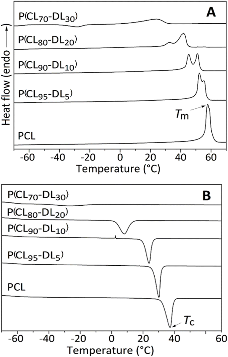Fig. 7 Heating (A) and cooling (B) DSC traces of the PCL and P(CL–DL) copolymers.

Fig. 8 XRD patterns of PCL and P(CL–DL) copolymers.

3.3 Thermal properties and morphology of composites

The thermal properties of composites (series I, II and III) were studied by TGA and DSC. The TGA thermograms (ESI, Fig. S2†) show that the thermal stability of composites is, in general, higher by few degrees than that of the unfilled polymers. On the other hand, the DSC traces show that the endotherms become wider and less intense in going from series I to series III (Fig. 9). They also show that CNF and CB have a different effect on the thermal behavior of copolymers.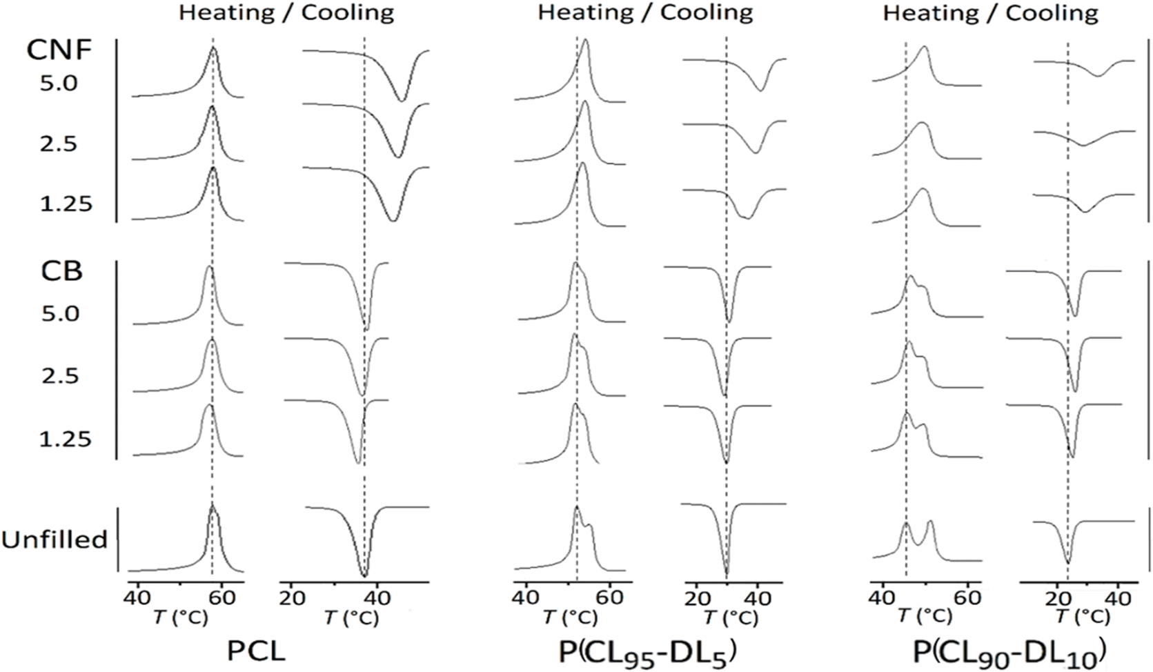

Fig. 9 DSC endo (up) and exotherms (down) for the composites of the series I: PCL/(CB or CNF), series II: P(CL₉₅–DL₅)/(CB or CNF), and series III: P(CL₉₀–DL₁₀)/(CB or CNF). The endo and exotherms of the neat or unfilled PCL, P(CL₉₅–DL₅) and P(CL₉₀–DL₁₀) polymers are included (bottom).

For P(CL₉₅–DL₅)/CNF and P(CL₉₀–DL₁₀)/CNF the endotherm (one single peak) is shifted to a higher temperature as compared with the pristine copolymers, suggesting that the polymer crystals become thicker and/or more perfect.⁴⁵ In a different way, the endotherm of P(CL₉₅–DL₅)/CB and P(CL₉₀–DL₁₀)/CB displays two maxima; the low-temperature one indicates that less perfect and/or thin crystals are formed. Thermograms also show that the CNF have a strong nucleation effect, which is reflected in a marked up-shift of T_c. For some of the P(CL–DL)/CNF nanocomposites, T_c is around 10 °C higher than that shown by the neat polymer (Table 4). For polymers filled with CB, the nucleation effect is rather limited with T_c up-shifts of only 2.5 °C or less. In Table 4, it can be seen that the crystallization degree of the composites remained similar to that of the neat polymers, except for the PCL/CB composites for which X_c decreases by around 20%. It should be reminded that the thermal diffusivity depends on the crystalline order in the bulk and around nanoparticles, as will be discussed later in this manuscript.

Table 4 Thermal and electrical properties of composites

	Tc (°C)	Tm (°C)	ΔHm (J g^−1)	Xc (%)	α (mm^2 s^−1)	k (W m^−1 K^−1)	VR (Ω cm)	σ (S cm^−1)
Series I
PCL	37.2	57.8	73.5	52.7	0.06	0.21	1 × 10^12	1 × 10^−13
PCL/CB1.25	35.8	57.1	57.8	41.9	0.13	0.23	3 × 10^12	4 × 10^−13
PCL/CB2.5	36.7	57.6	58.6	43.1	0.17	0.34	4 × 10^12	2 × 10^−13
PCL/CB5.0	37.8	57.0	58.8	44.4	0.19	0.40	3 × 10^12	3 × 10^−13
PCL/CNF1.25	43.8	58.0	70.8	51.4	0.20	0.34	6 × 10^12	2 × 10^−13
PCL/CNF2.5	45.1	57.7	70.7	51.9	0.24	0.45	3 × 10^12	4 × 10^−13
PCL/CNF5.0	45.9	58.1	66.0	49.8	0.30	0.55	5 × 10^12	2 × 10^−13
Series II
P(CL95–DL5)	30.1	52.3	57.7	42.6	0.13	—	2 × 10^12	6 × 10^−13
P(CL95–DL5)/CB1.25	30.2	51.9	54.9	41.0	0.16	0.35	2 × 10^12	5 × 10^−13
P(CL95–DL5)/CB2.5	29.5	51.7	53.5	40.5	0.19	0.37	3 × 10^12	3 × 10^−13
P(CL95–DL5)/CB5.0	31.2	51.9	52.4	40.7	0.16	0.33	4 × 10^11	3 × 10^−12
P(CL95–DL5)/CNF1.25	37.1	53.6	53.7	40.2	0.17	0.37	4 × 10^12	3 × 10^−13
P(CL95–DL5)/CNF2.5	39.5	54.2	56.4	42.7	0.22	0.45	4 × 10^12	2 × 10^−13
P(CL95–DL5)/CNF5.0	41.1	54.4	57.1	44.3	0.15	0.49	3 × 10^9	4 × 10^−10
Series III
P(CL90–DL10)	23.9	45.3	48.3	37.0	0.15	0.17	3 × 10^12	3 × 10^−13
P(CL90–DL10)/CB1,25	25.3	45.7	47.5	36.8	0.13	0.29	4 × 10^11	3 × 10^−12
P(CL90–DL10)/CB2.5	26.2	46.1	46.4	36.4	0.16	0.30	5 × 10^11	2 × 10^−12
P(CL90–DL10)/CB5.0	26.1	46.5	44.2	35.6	0.13	0.29	3 × 10^11	3 × 10^−12
P(CL90–DL10)/CNF1.25	29.4	49.3	44.8	34.6	0.11	0.28	2 × 10^11	6 × 10^−13
P(CL90–DL10)/CNF2.5	28.4	49.3	45.1	35.3	0.14	0.31	9 × 10^8	1 × 10^−9
P(CL90–DL10)/CNF5.0	33.2	49.8	45.4	36.6	0.11	0.29	1 × 10^7	1 × 10^−7

---

One of the most relevant characteristics of nanoparticles is their high surface-to-volume ratio, which may allow the transfer of properties to polymers at low particle contents.⁴⁶ Such transfer occurs when the polymer-particle interaction is good and, also, when particles are fully distributed and homogeneously dispersed in the polymer matrix. In this work, melt processing has shown to be a suitable mixing method for the distribution and dispersion of nanoparticles. By SEM studies, it was observed that both CB and CNF are fairly well dispersed in the continuous phase. Of the all captured SEM micrographs, only two were selected as representatives: one for polymers filled with CB (Fig. 10A) and other for those filled with CNF (Fig. 10B). In both micrographs, a good contact between polymer and particles is observed. The first shows “CB particles” and some “aggregates of few CB particles” in contact and enveloped with the matrix, whereas the second one shows single fibers entering and embedding in the polymer phase. Three additional SEM images, showing that carbon nanofibers are well dispersed in the polymer matrix, are included in ESI (Fig. S3).† A comparative analysis was made with reported SEM micrographs of polypropylene/CNF nanocomposites (images not shown here) that show cavitation as a consequence of poor compatibility.⁴⁷ PP is no-polar whereas the P(CL–DL) copolymers possess polar groups that can make the polymer-particle interaction possible. It should be reminded that both CB and CNF have structural and chemical defects to which the polymer chains can adhere.³¹ One possible mechanism may involve oxygen-containing functional groups of particles interacting with the ester groups of the polymer chains. Also, structural defects of particles could be anchoring sites for polymer chains. It is to point out that the co-rotating twin-screw micro extruder (Xplore model MC 15) is widely used for research at lab-scale, but it has some limitations as compared with other mixing machines. For future works some strategies might be implemented to improve dispersion, like using ultrasound during mixing, modify the nanoparticles with functional groups increase polymer-particle compatibility, and use performed mixing machines, among others.

Fig. 10 SEM micrographs of P(CL₉₀–DL₁₀)/CB₅ (A) and P(CL₉₀–DL₁₀)/CNF₅ (B).

3.4 Thermal and electrical properties of composites

The thermal and electrical conductivities of materials of the series I, II and III are listed in Table 4. It can be noticed that, the thermal conductivity of composites is, in general, higher than that of the unfilled polymers. Series I show a remarkable value of 0.55 W m⁻¹ K⁻¹, which is ∼160% higher than that measured for the unfilled PCL (0.21 W m⁻¹ K⁻¹). Series II reaches a maximum k value of 0.49 W m⁻¹ K⁻¹, whereas series III attains only 0.31 W m⁻¹ K⁻¹. Apart from these particular data, one can see that k increases with increasing the content of nanoparticles, although for some of the composites with 5 wt% of nanoparticles this tendency is inverted by a possible re-agglomeration of particles.⁴⁸ It can also be noticed in Table 4 that k of the P(CL–DL)-based composites is smaller than that of the PCL-based ones. This difference might be due to extended amorphous zones in the P(CL–DL) matrix through which phonons can hardly move.⁴⁹ Another observation is that for series I and II, CNF are clearly superior to CB nanoparticles to enhance the thermal conductivity of polymers. The high aspect ratio of CNF facilitates the particle–particle contact that, in combination with crystalline zones in the bulk and around nanoparticles (CNF showed a good nucleation effect), makes the heat transfer easier. A possible additional reason is that polymer crystals are more perfect (according to T_m up-shift in the DSC traces, Fig. 9) in the CNF-based composites than in the CB-based ones, and therefore phonons may be less dispersed in the former. For series III, no real difference in k between the CB and CNF-based composites is appreciated; the abundant amorphous zones in the P(CL₉₀–DL₁₀) copolymer might be impeding the heat transfer across the samples.

The electrical conductivity showed a different scenario (Table 4). For the CB-based composites, no enhancement in σ was observed, whereas for the CNF-based ones, significant differences were found between the three series. For series I, σ remained low and similar to that of the unfilled PCL (10⁻¹³ S cm⁻¹) and for series II and III, σ reached a value of up to 10⁻¹⁰ and 10⁻⁷ S cm⁻¹, respectively. The last one is six orders of magnitude higher than that shown by the neat P(CL₉₀–DL₁₀) copolymer. This result seems to indicate that the content of DL is in favor and not against σ, which is contrary to what was seen with k results. The electron transport occurs only when conductive particles are connected to each other into continuous networks (percolation), allowing electrons to move across the matrix. The high aspect ratio of CNF is favorable to the formation of conducting networks at low particle contents. The main electrical conduction mechanism in polymer nanocomposites consists of the transport of electrons through conducting particles placed close enough to allow electron tunneling happen.^50,51 Electron conducting networks are likely to be formed only in the P(CL–DL)/CNF nanocomposites (series II and III), which, according to DSC and XRD results, are less crystalline than the PCL/CNF ones (series I). The dependence of σ on crystallinity in nanocomposites is not so simple to explain as both direct and inverse effects have been reported. Crystals homogeneously nucleated can push the conducting particles to the amorphous zones, allowing them to concentrate and develop percolated structures. This is known as crystal-induced volume exclusion effect.⁵² However, nanoparticles with high nucleation capability develop polymer crystal structures on their surface, increasing thus the contact resistance, which is detrimental for the transport of charge carriers.⁴⁵ For PCL/CNF nanocomposites, it is possible that thick crystalline zones, growing from the surface of CNF, form barriers for the electron transfer, whereas for P(CL–DL)/CNF nanocomposites, thin and imperfect crystalline zones around CNFs, makes the CNFs approach each other (tunneling distance), making possible the electron tunneling.⁵³ From these results it is clear that the higher electrical conductivity of the copolymer P(CL–DL)/CNF compared to P(CL–DL)/CB is due to the high aspect ratio of CNFs, which can form a conductive network at lower concentration than CB, although the conductivity is likely to be dependent on the crystallinity at the polymer-CNF interface. The higher electrical conductivity in P(CL–DL)/CNF is also due to the fact that electrons move along the nanofiber before being transferred to a neighboring CNF in the percolated network.

When a sinusoidal or time-varying electric field is applied across a dielectric material, permittivity becomes a complex number. The real part of the relative permittivity (dielectric constant) is related to the energy stored in the material whereas the imaginary part (dielectric losses) is associated with the polarization and orientation of dipoles.⁵⁴ Nanocomposites showing high ε′ and low tan δ are desired in applications involving charge transport and storage, like capacitors, actuators and sensors. These two conditions (high ε′ and low tan δ) can be observed when the concentration of particles is near percolation.⁵⁵ It was proposed that the marked increase of ε′ near percolation is due to the formation of a large number of mirco capacitors, which are thought to be formed of conducting particles separated by a thin polymeric layer.⁵⁶ In this work, ε′ and tan δ were measured in a 20 Hz to 2 MHz frequency range and results are plotted in Fig. 11 and 12, respectively. In each plot, the type (CB or CNF) and amount (1.25, 2.5 or 5wt%) of nanoparticles are maintained constant. This allows us to appreciate the effect of the DL mol% on ε′ and tan δ. In the ε′ versus frequency plots (Fig. 11) a slight increase of ε′ is observed when the DL mol% in the copolymer increases. This may signify that in the P(CL–DL)-based nanocomposites more charge carriers (energy) migrate and accumulate at the filler–matrix interface, as compared with the PCL-based ones whose ε′ value remains unchanged in the all-frequency range. From one plot to the other, it can be noted that ε′ of the P(CL–DL)-based nanocomposites increases with the content of nanoparticles. A marked rise is observed only for the P(CL₉₅–DL₅)/CNF₅ and P(CL₉₀–DL₁₀)/CNF₅ nanocomposites, which, at low frequency, reached an ε′ value of ∼35. These two nanocomposites are near the percolation threshold (see Table 4) where a marked enhancement of ε′ is expected to occur.⁵⁷

Fig. 11 Dielectric constant – frequency plots of composites of the series 1 (solid lines), series II (dash lines) and series (III, dash dot lines).

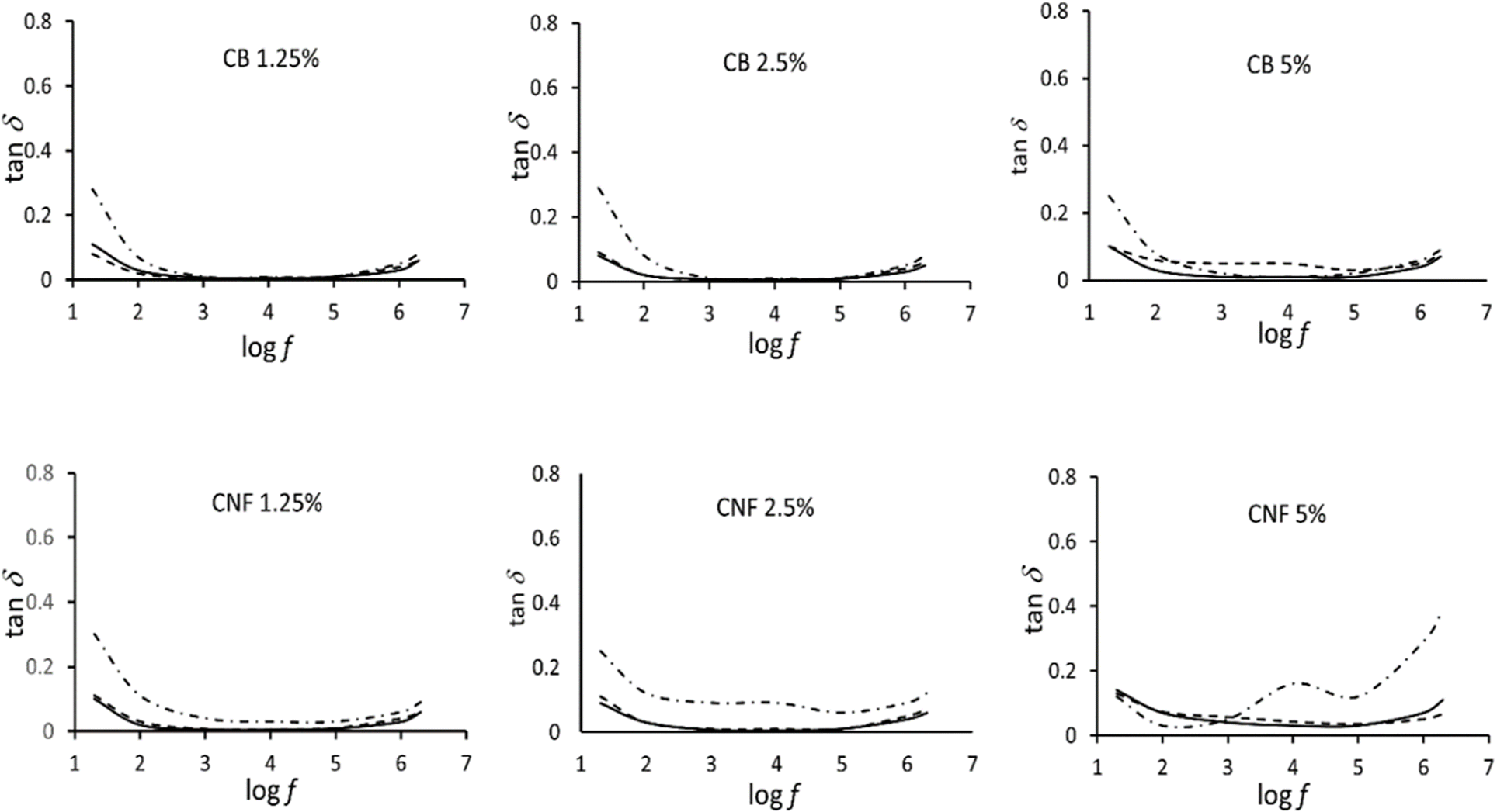Fig. 12 Dielectric losses – frequency plots of composites of series 1 (solid lines), series II (dash lines), and series (III, dash-dot lines).

For the CB-based composites, ε′ remained rather low (≤6) because they are far from percolation. It should be mentioned that for the unfilled or neat polymers (not included in plots) ε′ remained low (∼1.8) in all the frequency range; their curves were omitted in Fig. 11 because most of them appeared overlapped with those of the nanocomposites containing 1.25wt% of nanoparticles. On the other hand, the tan δ – frequency plots showed almost no-variation neither on the DL mol% nor on the content of nanoparticles (Fig. 12). Only a slight increase (up to 0.37) was observed for the P(CL₉₀–DL₁₀)/CNF₅ nanocomposite. The sudden enhance of ε′ (up to 35) while the tan δ remains low (<0.4) suggests us that this sample is near percolation. The introduction of the ε-decalactone comonomer in PCL is therefore a good strategy to tune the thermal and electrical properties of PCL-based nanocomposites.

There is a range of commercial products especially designed for the thermal management of modern electronic devices. Most of them are high thermal conductive composites prepared either with high amounts of nanoparticles (10 to 60 wt%) or using elaborated processing techniques.⁵⁸ However, not all polymer composites need to be high thermal conductive materials to be used for this purpose. For instance, acrylic-based materials with k values of 0.5 to 0.8 W m⁻¹ K⁻¹ are being used as adhesives and pads in electronic components.⁵⁹ The thermal performance of the PCL-based composites here prepared and studied is comparable to such commercial products used in electronic components. Aliphatic polyesters, like PCL, are in general more expensive (twice as much or more) than conventional plastics but, in modern times, the cost of polymers for the electronic industry may also consider the environmental impact as well as the economy gains in the end-of-life management of the e-waste.⁶⁰ Despite their higher cost, aliphatic polyesters have potential use in the electronic industry, especially in the light of the green chemistry and sustainability concepts.

Finally, the PCL/CNF_2.5wt% composite was exposed to a composting environment to evaluate its degree of disintegration. Pure PCL was also tested as reference. Tests were performed using the ISO20200:2015 standard testing for plastic disintegration under a compositing environment (thermophilic incubation process at 58 ± 2 °C).

In this biodegradation test, the degree of disintegration is measured as wt% loss of a material at different time intervals (30, 60 and 90 days). Composting is a biological decomposition of biowaste in the presence of oxygen and under controlled conditions by the action of micro- and macro-organisms.⁶⁰ Results show that, after 90 days, the registered weight loss for PCL and PCL/CNF_2.5wt% samples are 95.5 and 90%, respectively. This result is comparable to that reported by Kalita et al. (∼90wt% in 90 days) for the disintegration of PCL under a composting environment.⁶¹ The slightly lower weight loss registered for the polymer composite suggests that the CNFs have almost no effect on the polymer disintegration.

4. Conclusions

PCL and PCL–DL copolymers were synthesized via ring opening polymerization. They were then combined (melt mixing) with low contents of carbon black or carbon nanofibers and resulting composites showed enhanced thermal (with both CB and CNF) and electrical (only with CNF) conductivities that reached a value of up to 0.55 W m⁻¹ K⁻¹ and 10⁻⁷ S cm⁻¹, respectively. The DL monomer had a detrimental effect on the thermal conductivity due to the increase on the amorphous phase, which is unfavorable for the transport of phonons. A contrary effect of the DL monomer was observed for the electrical conductive and it was explained in terms of thin crystalline zones around nanofibers that allow the formation of a percolated or near percolated network for the electron transport. The dielectric constant of polymers was enhanced with increasing both the DL and nanoparticles contents. A marked enhancement was observed only for the P(CL₉₀–DL₁₀)/CNF_2.5 and P(CL₉₀–DL₁₀)/CNF_5.0 nanocomposites which attained (or are near) percolation. One of the nanocomposites showed a sudden enhance of ε′ (up to 35) while its tan δ remained low (<0.4) suggesting that this sample is near percolation. Results on both thermal and electrical properties are quite satisfactory, although much work is still needed to overcome limitations such as lack of control over the CL/DL molar ratio and poor particle dispersion. Future works may involve some new synthesis strategies of polymers and the use of more performed processing machines (compounders). Modification of particles to improve compatibility may perhaps be considered. For industrial applications, it would be necessary to do pilot plant experiments for both polymer synthesis and polymer/particle mixing. The molar composition control in copolymers can be achieved by controlling the monomer addition along the polymerization reaction (semi-continuous reaction), taking into account that the reactivity of CL is much higher to that of the DL monomer. Concerning the particle dispersion, performed industrial mixing machines (intensive mixing extruders) need to be used. Finally, some of the nanocomposites here prepared have thermal and electrical conductive (or dissipative) capacities that may be useful for heat dissipation and electrostatic charges releasing in sustainable flexible electronic devices.

Data availability

The data that support the findings of this study are not available.

Author contributions

DIMB: investigation, project administration, validation, writing original draft; DNR: conceptualization, writing original draft, review and supervision; HRLG: conceptualization, funding acquisition, project administration, and MAJT: investigation, conceptualization, validation, writing original draft.

Conflicts of interest

The authors declare no conflict of interest.

Acknowledgements

Authors acknowledge the technical support of Martha Roa-Luna, Maricela García-Zamora, Myrna Salinas-Hernández, Guadalupe Méndez-Padilla, Jesús Alfonso Mercado, Janett Valdéz-Garza, Alejandro Díaz Elizondo and Ricardo Mendoza Carrizales from CIQA. MAJT acknowledges the financial support (A1-S-34241) from the Consejo Nacional de Humanidades Ciencia y Tecnología (CONAHCYT) of Mexico through the Postdoctoral grants program and financial support of the CONAHCYT through the Basic Science Projects A1-S-34241 and 320806.

References

1. J. C. Prata, The environmental impact of e-waste microplastics: A systematic review and analysis based on the driver-pressure-state-impact-response (DPSIR) framework, Environments, 2024, 11, 30.
2. K. Liu, Q. Tan, J. Yu and M. Wang, A global perspective on e-waste recycling, Circular Economy, 2023, 2, 100028.
3. V. R. Feig, H. Tran and Z. Bao, Biodegradable polymeric materials in degradable electronic devices, ACS Cent. Sci., 2018, 4, 337.
4. Q. Sun, B. Qian, K. Uto, J. Chen, X. Liu and T. Minari, Functional biomaterials towards flexible electronics and sensors, Biosens. Bioelectron., 2018, 119, 237.
5. J. Kwon, C. DelRe, P. Kang, A. Hall, D. Arnold, I. Jayapurna, L. Ma, M. Michalek, R. O. Ritchie and T. Xu, Conductive ink with circular life cycle for printed electronics, Adv. Mater., 2022, 34, 2202177.
6. D. I. Medellín-Banda, D. Navarro-Rodríguez, M. A. De Jesús Téllez, F. Robes-González and H. R. López-González, Poly(butylene succinate). Functional nanocomposite materials and applications, in Green Based Nanocomposite Materials and Applications, ed. F. Ávalos-Belmontes et al., Book Series Engineering Materials, Springer, 2023, ch. 13, p. 251.
7. J. R. Dias, A. Sousa, A. Augusto, P. J. Bártolo and P. L. Granja, Electrospun polycaprolactone (PCL) degradation: An in vitro and in vivo study, Polymers, 2022, 14, 3397.
8. M. Bartnikowski, T. R. Dargaville, S. Ivanovski and D. W. Hutmacher, Degradation mechanisms of polycaprolactone in the context of chemistry, geometry and environment, Prog. Polym. Sci., 2019, 96, 1.
9. Z. Sun, B. Chen, Y. Wang, X. Tuo, Y. Gong and J. Guo, Study on metal alloy-reinforced polycaprolactone 3D printed composites for electromagnetic protection, Compos. Sci. Technol., 2022, 225, 109516.
10. F. Chen, L. Xu, Y. Tian, A. Caratenuto, X. Liu and Y. Zheng, Electrospun polycaprolactone nanofiber composites with embedded carbon nanotubes/nanoparticles for photo-thermal absorption, ACS Appl. Nano Mater., 2021, 4, 5230.
11. N. A. Masarra, M. Batistella, J. C. Quantin, A. Regazzi, M. F. Pucci, R. El Hage and J. M. Lopez-Cuesta, Fabrication of PLA/PCL/graphene nanoplatelet (GNP) electrically conductive circuit using the fused filament fabrication (FFF) 3D printing technique, Materials, 2022, 15, 762.
12. M. Abdulrhman, A. Zhakeyev, C. M. Fernández-Posada, F. P. W. Melchels and J. Marques-Hueso, Routes towards manufacturing biodegradable electronics with polycaprolactone (PCL) via direct light writing and electroless plating, Flexible Printed Electron., 2022, 7, 025006.
13. G. Damonte, A. Vallin, D. Battegazzore, A. Fina and O. Monticelli, Synthesis and characterization of a novel star polycaprolactone to be applied in the development of graphite nanoplates-based nanopapers, React. Funct. Polym., 2021, 167, 105019.
14. K. Li, D. Battegazzore, R. A. Pérez-Camargo, G. Liu, O. Monticelli, A. J. Müller and A. Fina, Polycaprolactone adsorption and nucleation onto graphite nanoplates for highly flexible, thermally conductive, and thermomechanically stiff nanopapers, ACS Appl. Mater. Interfaces, 2021, 13, 59206.
15. J. Cheng, L. Wang, J. Huo, H. Yu, Q. Yang and L. Deng, Preparation and conductive properties of polycaprolactone-grafted carbon black nanocomposites, J. Appl. Polym. Sci., 2009, 114, 2700.
16. M. Hou, Y. Feng, S. Yang and J. Wang, Multi-hierarchically structural polycaprolactone composites with tunable electromagnetic gradients for absorption-dominated electromagnetic interference shielding, Langmuir, 2023, 39, 6038.
17. S. Farzamfar, M. Salehi, S. M. Tavangar, J. Verdi, K. Mansouri, A. Ai, Z. V. Malekshahi and J. Ai, A novel polycaprolactone/carbon nanofiber composite as a conductive neural guidance channel: an in vitro and in vivo study, Prog. Biomater., 2019, 8, 239.
18. S. Ghaziof and M. Mehdikhani-Nahrkhalaji, Preparation, characterization, mechanical properties and electrical conductivity assessment of novel polycaprolactone/multi-wall carbon nanotubes nanocomposites for myocardial tissue engineering, Acta Phys. Pol. A, 2017, 131, 428.
19. M. Petousis, L. Tzounis and N. Vidakis, A Review on the functionality of nanomaterials in 2d and 3d additive manufacturing, Res. Dev. Mater. Sci., 2020, 14, 00083.
20. A. Cruz-Aguilar, D. Navarro-Rodríguez, O. Pérez-Camacho, S. Fernández-Tavizón, C. A. Gallardo-Vega, M. García-Zamora and E. Díaz Barriga-Castro, High density polyethylene/graphene oxide nanocomposites prepared via in situ polymerization: Morphology, thermal and electrical properties, Mater. Today Commun., 2018, 16, 232.
21. D. I. Medellín-Banda, D. Navarro-Rodríguez, S. Fernández-Tavizón, C. A. Ávila-Orta, G. Cadenas-Pliego and V. E. Comparán-Padilla, Enhancement of the thermal conductivity of polypropylene with low loadings of CuAg alloy nanoparticles and graphene nanoplatelets, Mater. Today Commun., 2019, 21, 100695.
22. H. Tian, F. Wu, P. Chen, X. Peng and H. Fang, Microwave-assisted in situ polymerization of polycaprolactone/boron nitride composites with enhanced thermal conductivity and mechanical properties, Polym. Int., 2020, 69, 635.
23. S. Park and R. S. Ruoff, Chemical methods for the production of graphenes, Nat. Nanotechnol., 2009, 4, 217.
24. H. J. Choi, M. S. Kim, D. Ahn, S. Y. Yeo and S. Lee, Electrical percolation threshold of carbon black in a polymer matrix and its application to antistatic fibre, Sci. Rep., 2019, 9, 6338.
25. X. Zhang, S. Hu, S. Huang, Y. Zhou, W. Zhang, C. Yang, C. Yao, X. Dong, Q. Zhang, M. Wang, J. Hu, Q. Li and J. He, Structure-performance relationship of polypropylene/elastomer/carbon black composites as high voltage cable shielding layer, Composites, Part A, 2024, 185, 108334.
26. T. Villmow, B. Kretzschmar and P. Pötschke, Influence of screw configuration, residence time, and specific mechanical energy in twin-screw extrusion of polycaprolactone/multi-walled carbon nanotube composites, Compos. Sci. Technol., 2010, 70, 2045.
27. D. K. Lee, J. Yoo, H. Kim, B. H. Kang and S. H. Park, Electrical and thermal properties of carbon nanotube polymer composites with various aspect ratios, Materials, 2022, 15, 1356.
28. C. Huang, X. Qian and R. Yang, Thermal conductivity of polymer and polymer nanocomposites, Mater. Sci. Eng., R, 2018, 132, 1.
29. T. Khan, M. S. Irfan, M. Ali, Y. Dong, S. Ramakrishna and R. Umer, Insights to low electrical percolation thresholds of carbon-based polypropylene nanocomposites, Carbon, 2021, 176, 602.
30. J. Gopinathan, M. M. Pillai, V. Elakkiya, R. Selvakumar and A. Bhattacharyya, Carbon nanofillers incorporated electrically conducting poly ε-caprolactone nanocomposite films and their biocompatibility studies using MG-63 cell line, Polym. Bull., 2016, 73, 1037.
31. L. Guadagno, M. Raimondo, V. Vittoria, L. Vertuccio, K. Lafdi, B. De Vivo, P. Lamberti, G. Spinelli and V. Tucci, The role of carbon nanofiber defects on the electrical and mechanical properties of CNF-based resins, Nanotechnol, 2013, 24, 305704.
32. F. Wu, S. Chen, X. Tang, H. Fang, H. Tian, D. Li and X. Peng, Thermal conductivity of polycaprolactone/three-dimensional hexagonal boron nitride composites and multi-orientation model investigation, Compos. Sci. Technol., 2020, 197, 108245.
33. A. Abdal-hay, M. Taha, H. M. Mousa, M. Bartnikowski, M. L. Hassan, M. Dewidar and S. Ivanovski, Engineering of electrically-conductive poly(ε-caprolactone)/multi-walled carbon nanotubes composite nanofibers for tissue engineering applications, Ceram. Int., 2019, 45, 15736.
34. K. Saeed and S. Y. Park, Preparation and properties of multiwalled carbon nanotube/polycaprolactone nanocomposites, J. Appl. Polym. Sci., 2007, 104, 1957.
35. Y. D. Shi, M. Lei, Y. F. Chen, K. Zhang, J. B. Zeng and M. Wang, Ultralow percolation threshold in poly(L-lactide)/poly(ε-caprolactone)/multiwall carbon nanotubes composites with a segregated electrically conductive network, J. Phys. Chem. C, 2017, 121, 3087.
36. Y. F. Chen, Y. J. Tan, J. Li, Y. B. Hao, Y. D. Shi and M. Wang, Graphene oxide-assisted dispersion of multi-walled carbon nanotubes in biodegradable poly(ε-caprolactone) for mechanical and electrically conductive enhancement, Polym. Test., 2018, 65, 387.
37. B. G. V. Basheer, J. J. George, S. Siengchin and J. Parameswaranpillai, Polymer grafted carbon nanotubes—Synthesis, properties, and applications: A review, Nano-Struct. Nano-Objects, 2020, 22, 100429.
38. E. Díaz, J. León, A. Murillo-Marrodán, S. Ribeiro and S. Lanceros-Méndez, Influence of rGO on the crystallization kinetics, cytotoxicity, and electrical and mechanical properties of poly(L-lactide-co-ε-caprolactone) scaffolds, Materials, 2022, 15, 7436.
39. C. G. Pitt, C. G. Chasalow, Y. M. Hibionada, D. M. Klimas and A. Schindler, Aliphatic polyesters. The degradation of poly(ε-caprolactone) in vivo, J. Appl. Polym. Sci., 1981, 26, 3779.
40. S. Thongkham, J. Monot, B. Martin-Vaca and D. Bourissou, Simple in-based dual catalyst enables significant progress in ε-decalactone ring-opening (co)polymerization, Macromolecules, 2019, 52, 8103.
41. G. Ramos-Durán, A. C. González-Zarate, F. J. Enríquez-Medrano, M. Salinas-Hernández, M. A. De Jesús-Téllez, R. Díaz de León and H. R. López-González, Synthesis of copolyesters based on substituted and non-substituted lactones towards the control of their crystallinity and their potential effect on hydrolytic degradation in the design of soft medical devices, RSC Adv., 2022, 12, 18154.
42. F. Robles-González, T. Rodríguez-Hernández, A. S. Ledezma-Pérez, R. Díaz de León, M. A. De Jesús-Téllez and H. R. López-González, Development of biodegradable polyesters: Study of variations in their morphological and thermal properties through changes in composition of alkyl-substituted (ε-DL) and non-substituted (ε-CL, EB, L-LA) monomers, Polymers, 2022, 14, 4278.
43. P. Olsén, T. Borke, K. Odelius and A. C. Albertsson, ε-Decalactone: A thermoresilient and toughening comonomer to poly(L-lactide), Biomacromolecules, 2013, 14, 2883.
44. B. Zou, Y. Zhan, X. Xie, T. T. Zhang, R. Qiua and F. Zhu, Synthesis of ultrahigh-molecular-weight ethylene/1-octene copolymers with salalen titanium(IV) complexes activated by methyaluminoxane, RSC Adv., 2022, 12, 11715.
45. J. Wang, Y. Kazemi, S. Wang, M. Hamidinejad, M. B. Mahmud, P. Potschke and C. B. Park, Enhancing the electrical conductivity of PP/CNT nanocomposites through crystal-induced volume exclusion effect with a slow cooling rate, Composites, Part B, 2020, 183, 107663.
46. K. Y. Lau and M. A. Piah, Polymer Nanocomposites in High Voltage Electrical Insulation Perspective: A Review, Malays. Polym. J., 2011, 6, 58.
47. C. A. Covarrubias-Gordillo, J. E. Rivera-Salinas, H. A. Fonseca-Florido, C. A. Ávila-Orta, F. J. Medellín-Rodríguez, D. I. Medellín-Banda and P. Pérez-Rodríguez, Enhancement of polypropylene mechanical behavior by the synergistic effect of mixtures of carbon nanofibers andgraphene nanoplatelets modified with cold propylene plasma, J. Appl. Polym. Sci., 2023, 140, e53957.
48. T. Wang, B. Song, K. Qiao, Y. Huang and L. Wang, Effect of dimensions and agglomerations of carbon nanotubes on synchronous enhancement of mechanical and damping properties of epoxy nanocomposites, Nanomaterials, 2018, 8, 996.
49. Z. Han and A. Fina, Thermal conductivity of carbon nanotubes and their polymer nanocomposites: A review, Prog. Polym. Sci., 2011, 36, 914.
50. Y. Zare and K. Y. Rhee, A simple methodology to predict the tunneling conductivity of polymer/CNT nanocomposites by the roles of tunneling distance, interphase and CNT waviness, RSC Adv., 2017, 7, 34912.
51. R. Razavi, Y. Zare and K. Y. Rhee, A two-step model for the tunneling conductivity of polymer carbon nanotube nanocomposites assuming the conduction of interphase regions, RSC Adv., 2017, 7, 50225.
52. H. Quan, S. J. Zhang, J. L. Qiao and L. Y. Zhang, The electrical properties and crystallization of stereocomplex poly(lactic acid) filled with carbon nanotubes, Polymer, 2012, 53, 4547–55.
53. Y. Zare and K. Y. Rhee, Calculation of the electrical conductivity of polymer nanocomposites assuming the interphase layer surrounding carbon nanotubes, Polymers, 2020, 12, 404.
54. J. C. Pandey and M. Singh, Dielectric polymer nanocomposites: Past advances and future prospects in electrical insulation perspective, Spec. Polym., 2021, 2, 236.
55. C. W. Nan, Y. Shen and J. Ma, Physical properties of composites near percolation, Annu. Rev. Mater. Res., 2010, 40, 131.
56. M. J. Jiang, Z. M. Dang, M. Bozlar, F. Miomandre and J. Bai, Broad-frequency dielectric behaviors in multiwalled carbon nanotube/rubber nanocomposites, J. Appl. Phys., 2009, 106, 084902.
57. M. Arjmand, M. Mahmoodi, S. Park and U. Sundararaj, An innovative method to reduce the energy loss of conductive filler/polymer composites for charge storage applications, Compos. Sci. Technol., 2013, 78, 24.
58. J. Wang, L. Hu, W. Li, Y. Ouyang and L. Bai, Development and perspectives of thermal conductive polymer composites, Nanomaterials, 2022, 12, 3574.
59. https://converting-tasm.pl/en/tesa_en/thermal-conductive-solutions-thermal-pads.
60. R. Mouhoubi, M. Lasschuijt, S. Ramon Carrasco, H. Gojzewski and F. R. Wurm, End-of-life biodegradation? how to assess the composting of polyesters in the lab and the field, Waste Manage., 2022, 154, 36.
61. N. K. Kalita, S. M. Bhasney, C. Mudenur, A. Kalamdhad and V. Katiyar, End-of-life evaluation and biodegradation of poly(lactic acid) (PLA)/polycaprolactone (PCL)/microcrystalline cellulose (MCC) polyblends under composting conditions, Chemosphere, 2020, 247, 125875.

---

Footnote

† Electronic supplementary information (ESI) available. See DOI: https://doi.org/10.1039/d4ra06932c

---