Hydration shell water surrounding citrate-stabilised gold nanoparticles

Abstract

The presence of foreign particles in an aqueous dispersion perturbs the water layers in the vicinity of the particles. These perturbed water molecules form what is known as the hydration shell and possess different structural attributes from those in the bulk dispersion. Here, Raman spectroscopy was utilised to study such hydration shells around citrate-stabilised gold nanoparticles. An aqueous dilution series of three sizes of gold nanoparticle samples was prepared. The hydration shell spectral response recovered by applying the multivariate curve resolution technique was compared against the spectra of the bulk phase. It could be inferred from the comparison that the hydration shell contains a less extensive hydrogen-bonding network with a smaller number of hydrogen-bonding interactions per molecule being possible than that in bulk. Control experiments and molecular dynamics simulations, using a modified Drude oscillator model for the gold, point to the presence of the gold surface to be the predominant factor behind influencing the hydrogen-bonding structure of the hydration shell water surrounding citrate-stabilised gold nanoparticles.

---

Introduction

Gold nanoparticle (Au NP) catalysed reactions in aqueous media^1,2 can potentially be relevant in our transformation towards a carbon-neutral energy sector. In order to understand all the underlying factors influencing the outcome of such reactions, specifically the reactions in which water is not just the medium but also a reactant itself, it is necessary to explore the effect of the presence of Au NPs on surrounding water layers. It is known that the extent of reactivities shown by Au NPs in water is influenced by the interfacial water molecules.³ In turn, the interfacial water itself is also expected to be influenced by the Au surface as a result of the prevailing interactions as is generally observed on metal/liquid interfaces.^4,5 When it comes to the NPs, given the fact that solvent restructuring takes place at the NP–solute interface,⁶ interfacial water should be expected to undergo a certain degree of structural changes while they are close to the Au NPs. In other words, solvation shell water, i.e., the water layers significantly perturbed by the presence of a solute (here, Au NPs), can be expected to have structural differences if compared to the bulk phase water. In the past, some theoretical reports have concentrated on studying Au NPs surrounded by water.^7,8 However, experimental studies probing the hydration shell around metallic NPs have been few and far between,^9,10 and no experimental study has likely been carried out yet, focusing on hydration shells around Au NPs in commonplace dispersions, ones that are used to prepare Au NPs for their multitude of applications.¹¹ Thus, it is worth experimentally studying the structural changes occurring in the hydration shells surrounding Au NPs in a usual, commonly used dispersion.

The Turkevich method,¹² which utilises citrate reduction of gold salt in combination with stabilisation of colloidal Au NPs by citrate anions, is widely used to synthesise Au NPs for their regular applications. So, citrate-stabilised Au NPs in an aqueous dispersion were chosen for the present investigation.

Furthermore, nanoparticle size can play a role in determining the extent of catalytic activities displayed by Au NPs,¹³ not just in non-aqueous media,¹⁴ but also in aqueous media.² Since greater catalytic activity could be associated with greater deformation of the solvation shell hydrogen-bonding environment, it was deemed interesting to check if any size dependent trend could be found in the way Au NPs influence their hydration shells. Therefore, three different sizes were chosen for this study.

Here, the effect of the presence of citrate-stabilised Au NPs (of three different nominal sizes) on the solvation shell water is examined experimentally. Having an extensive network of easily perturbed hydrogen-bonding, liquid water manifests significant changes in vibrational spectroscopic response, stemming from structural changes that lead to changes in water intermolecular interactions. Therefore, vibrational spectroscopic tools such as Raman spectroscopy present a powerful tool to study the water structure.

One of the challenging aspects of experimentally recovering a spectral response from the solvation shell is the fact that under usual circumstances, the number of solvent molecules forming the solvation shell is overwhelmingly inferior to the number of solvent molecules constituting the bulk. One approach to identify the changes in the spectral features arising due to the presence of the solute is to study the difference spectrum generated by subtracting the neat solvent spectrum from the solution spectrum. This approach has been employed in examining solvation shell water around silver nanoparticles using Raman spectroscopy,⁹ when the authors measured background spectra as well as spectra of aqueous dispersions of laser ablated silver NPs and used the spectral subtraction method on their way to derive their conclusions. Another innovative way to tackle the issue is exemplified by the work reported by Novelli et al.,¹⁰ in which hydration shell water around neutral and charged Au NPs embedded inside micellar formation was probed by modification of the water content in an organic solvent. It was possibly hypothesised by the authors that after drying the samples, the leftover water content being probed was exclusively the hydration shell water. Apart from these techniques, the multivariate curve resolution (MCR) method of data analysis^15–17 under physically meaningful constraints offers a powerful alternative that can be employed to distinguish the solute-correlated spectrum from the bulk solvent spectrum. The MCR approach has an added advantage, over the difference strategy, of being able to provide a complete spectral response of solute-correlated component which can be directly compared with the bulk solvent spectrum, allowing the possibility to observe them side by side, in order to gain useful insights. In addition, this method allows the user to study a system without any environmental modification around the solute. This enables investigation under conditions that better resemble commonplace use cases of the solute–solvent system under consideration. This approach can be referred to as “solvation shell spectroscopy” in general, in line with calling it “hydration shell spectroscopy”¹⁸ when the solvent is water. This approach has been successfully used in the past in conjunction with Raman^19–26 and infrared²⁷ spectral data gathered from aqueous systems.

In this work, Raman spectroscopic study of hydration shell water surrounding three different sizes of commercially procured, citrate-stabilised Au NPs is discussed. In order to reveal the influence of the presence of the Au NPs on water in the system, a dilution series with water was prepared and the gradual changes in spectral profiles were followed. The solute-correlated spectra were compared with the spectra for bulk phase liquids and conclusions were drawn about the state of the hydrogen-bonding network around the nanoparticles. Further experiments and classical molecular dynamics (MD) simulations were carried out to gain a better understanding of the origin of the observed differences between the bulk and the solute-correlated spectra.

Methods

The Raman spectra were recorded for a series of concentrations (number densities) of Au NPs. For this purpose, three types of citrate-stabilised spherical Au NP samples were purchased from Nanopartz Inc., USA (product numbers A11-10-ClT-DIH-1-25, A11-30-ClT-DIH-1-25, and A11-50-ClT-DIH-1-25, respectively, for NP diameters of 10, 30 and 50 nm). They were used as received.

UV-visible spectra for the three batches of the Au NPs were measured using a PerkinElmer Lambda 800 UV-visible spectrophotometer (see Fig. S1 in the ESI†).

Ultrapure water (Elga Purelab Plus UV) with an electrical resistivity of 18.2 MΩ cm was used in this work. All the references to water in the rest of this article should normally be taken to mean this quality of water. Three stock dispersions were prepared by diluting the supplied Au NP colloids with water and the respective concentration series were prepared by further diluting these stock dispersions with water. The stock dispersions were prepared by keeping the total approximate surface area of 30 nm and 50 nm NPs in each stock dispersion equal by adopting the crude assumptions that the NPs were all spheres and all the Au NPs had diameters of 10 nm (NP10), 30 nm (NP30) and 50 nm (NP50) for the respective samples. The concentration of NP10 was five times the concentration needed to keep the surface area identical to NP30 and NP50. This increase in the particle concentration was found to be necessary to have strong enough changes in the NP10 sample spectra, compared against the corresponding dispersing media spectra, so that detectable solute-correlated spectra, distinct from the noise level in the spectra, are obtained. The concentration series for each of the three batches of Au NPs comprised of 20%, 40%, 60%, 80% and 100% (V/V) strength, as calculated against the stock dispersions. The concerned properties and the dilution factors for the preparation of the stocks are presented in Table S1 in the ESI.†

The samples were divided into two sets, one for the spectroscopic measurements and the other for centrifugation. The samples in the latter set were subjected to centrifugation for 1 hour at 12 500 rpm using an Eppendorf centrifuge 5430. The supernatant liquids were collected and were considered to be the dispersing media for the respective NP samples. This protocol was tested, using UV-visible spectroscopy, to be satisfactory for adequate removal of Au NPs from the dispersing medium (Fig. S1†). The supernatant liquid separated from each of the samples was further measured under the same spectroscopic conditions as those used for the Au NP samples in the NP10, NP30 and NP50 series.

Additionally, to carry out an experiment to better understand the origin of the spectral features in the solute-correlated spectra obtained from the Au NP samples, several aqueous solutions of trisodium citrate dihydrate (Sigma-Aldrich, used without further purification) were prepared with different strengths (1, 5, 10, 100 and 1000 mM).

Raman spectral measurements

The Raman spectra were recorded using a LabRam confocal Raman spectroscopy instrument (Horiba Jobin Yvon, France). An Ar ion laser with an emission wavelength of 514.532 nm (ca. 514.5 nm), a 600 grooves per mm grating and an Olympus 10× objective (numerical aperture 0.25) were used in conjunction with a charge-coupled device (CCD) detector. Each of the spectra was collected for 5 seconds of integration time, averaged over 100 accumulations. The beam power at the position of the sample was around 15 mW for all the measurements. The spectra were corrected for the wavenumber shift by calibrating the position of the laser line to zero by fitting the laser line spectrum to a Gaussian function.

The Raman spectral profile of water varies with the change in temperature.^28–32 Therefore, it was deemed important to ensure stability and consistency in the temperature at which all the samples were to be measured. The Raman spectral measurements were carried out on samples contained in a cylindrical quartz glass cuvette with an outside shell for flow of water from the thermostat. A PT100 sensor was attached to the window of the outside shell and the temperature values were observed using a Greisinger GMH 3710 thermometer. In all subsequent references to recorded temperature in this article, the reading of this setup has been referred to. This temperature reading does not necessarily depict the temperature of the sample but if the measured temperature is stable, it can be inferred that the temperature of the sample is also stable and consistent throughout the experiments. The temperatures recorded during the measurements showed a variation within the range of 22.18 ± 0.05 °C.

For a control experiment to check the influence of slight temperature fluctuations on the lineshapes of the Raman spectra of aqueous samples, a series of Raman spectra of water were recorded with around 0.1 °C increment in temperature in the range of 21.75 to 22.73 °C average temperatures during the spectral measurements that were carried out under identical experimental conditions as employed for the NP samples and the corresponding dispersing media. These blank measurements were used to draw relevant inferences in section 10 of the ESI.†

In addition, Raman spectra were recorded for water and the citrate solutions (1, 5, 10, 100, and 1000 mM).

MCR analysis

The MCR as a linear algebraic method aims to express a data matrix D as the following linear transformation:

D = CS^T. (1)

In the present scenario, the data to be dealt with is spectroscopic. Therefore, in eqn (1), the input matrix D contains the area normalised Raman intensities in the selected window of wavenumbers. C is the concentration matrix, with columns carrying concentrations of each of the components across samples. S^T is the transposed spectra matrix, with rows carrying calculated spectra of each of the components.

To recover the weak solute-correlated signal buried beneath the strong bulk signal, MCR with an alternating least squares (ALS) algorithm was implemented using the open-source Python library pyMCR (version 0.5.2).³³ Starting from initial concentration guesses, “ordinary least squares” regression was used with “non-negativity” constraints on both concentration and spectral matrices. The pyMCR version 0.5.2 allowed fixing the concentration values of any component across all samples throughout all iterations. This work, however, required fixing the concentration values of all components in one of the samples. A minor adaptation (changing the type of the pyMCR parameter “c_fix” to Boolean array) enabled fixing the concentration of any component in a single sample (or potentially, multiple samples) while leaving the concentration values of that component in all other samples free to vary.

Data from 2650–3900 cm⁻¹ (O–H stretching region) were selected, with a linear baseline subtracted between the endpoints. Small negative values (close to the edges) generated due to noise were corrected with an intensity offset, ensuring a minimum positive value (10⁻³⁰⁰) in each spectrum. Following the established convention^19,34 for spectral pre-processing in MCR studies, all the spectra were normalised to the unit area to account for intensity variation from external factors such as laser power fluctuation or optical alignment variations.

In an MCR analysis, for a system comprising of n samples, there are n mathematically possible components that can contribute intensity to the measured resultant spectra. Here, the system was assumed to be a combination of two components: (1) bulk component and (2) solute-correlated component. Therefore, in the current study, all the spectral features in the NP sample spectra that are different from the spectrum of the bulk phase chosen for the MCR analysis would appear in the solute-correlated spectrum. The corresponding dispersing medium (supernatant liquid collected after centrifugation) was chosen to be the pure bulk component for every NP sample.

Each MCR analysis started with an initial concentration guess. For the bulk component, it was 1 in the dispersing medium and 0.98 in the NP sample and for the solute-correlated component, 0 and 0.02 respectively. Since prior knowledge about the system is not inherently required for MCR as a method to work,^15,35 the initial guesses need not be precise; nevertheless, realistic initial guesses and constraints lead to results that better describe the reality. However, for only a pair of spectral data, the choice of the initial guesses is not at all critical, as long as concentration guesses are of similar magnitude and the solute-correlated component is fixed at zero in the bulk-only spectrum. Here, as the dispersing medium contained only the bulk component, its component concentrations were fixed at 1 (bulk) and 0 (solute-correlated), while the component concentrations in the NP samples were allowed to vary.

Similar MCR analyses were conducted using water as the bulk spectrum, paired separately with the spectra of citrate solutions at 1, 5, 10, 100, and 1000 mM concentrations.

Classical molecular dynamics simulations

Classical MD simulations of the Au(111)-aqueous solution interface were performed at various prescribed concentrations (0 M, 0.1 M, 0.25 M, and 0.5 M) of sodium citrate, as well as the corresponding bulk simulation boxes, using the LAMMPS³⁶ simulation package. The choice of a classical, Lennard–Jones based approach was made to allow for sufficiently large simulation cells so as to have a sufficient number of citrate molecules (while still maintaining a sensible concentration) and long enough simulation times to obtain rigorous statistics.

It has previously been shown that while there is variation in exact ratios due to kinetic and thermal effects, the Au(111) facet makes up the majority of the Au NP surface, followed by the (100) facet.^37–39 This is in part due to the (111) facet having the lowest surface energy. Owing to this, and owing to the fact that the sizes of the Au NPs used in the experiments were large enough to render the local Au surface almost planar with regard to a molecule as small as water, the decision was made to run the simulation using a slab geometry of the Au(111) surface as a model system. It has been shown that the edges in NP geometry play an important role in their behaviour;⁸ however for the focus of this study, a simpler system is sufficient while also saving computational costs and simplifying the analysis of the trajectory.

In standard classical MD simulation, the particles are represented as hard non-polarisable spheres, optionally with a net charge in the case of an ion. While this approach can produce good and physically meaningful results, it leads to a radially symmetric potential that does not change under the influence of neighbouring particles/charges, rendering dynamic electron polarisation impossible to simulate. In the case of simulating Au NPs, this presents a fatal flaw, due to the importance of such effects in the interaction of the Au surface with both water and relevant solutes such as sodium citrate. A number of alternative models exist to account for these effects, such as a posteriori addition of a virtual charge plane,⁴⁰ or the representation of the gold particles as freely rotating dipoles of a fixed length.⁴¹

In this work, we employ a different approach based on the Drude oscillator⁴² previously developed by Geada et al.,⁴³ whereby gold atoms are represented as a “core” with a charge of +1.0 e, along with a “dummy electron” of charge −1.0 e and mass 1 a.u. (with the mass of the core correspondingly lowered). These are then connected by a harmonic bond with a rest length of 0 Å and a spring constant calculated to reproduce the polarisability of the gold atom from density functional theory (DFT) calculations to a first order. This approach has the crucial benefit of allowing for truly dynamic polarisation effects, and has since been widely used for the study of the Au surface with a variety of biomolecules and water.⁴⁴

For the solution, a flexible model based on modified CHARMM⁴⁵ parameters of the fully deprotonated citrate anion was chosen.⁴⁶ This model was developed to accurately reproduce the conformational and binding behaviour of the citrate anion with reference to Car–Parinello MD simulations⁴⁷ and has subsequently been proven effective in a wide variety of applications,^48,49 including the simulation of citrate on the Au surface⁵⁰ and Au NPs.⁵¹ In tandem, the 3-site rigid SPC/E water model⁵² was used, as while the citrate model was developed with the related flexible SPC/Fw model,⁵³ rigid water models have been shown to have better thermodynamic and structural properties.⁵⁴ The SPC/E model is rigid and overall charge neutral, but represents the water molecule dipole through fixed partial charges on both the oxygen and hydrogens, leading to overall charge neutrality while still producing preferable electrostatic and bulk properties.

The simulation boxes were prepared using an Au(111) gold slab generated using the Atomic Simulation Environment python package,⁵⁵ converted to the Drude oscillator model using in-house code following the parameterisation described by Geada et al.⁴³ The SPC/E molecule file was taken from the LAMMPS website, and the sodium citrate molecule file converted from GROMACS to LAMMPS parameters in-house, with the corresponding L-J parameters for the sodium cation being used; missing pair L-J parameters were generated through the arithmetic mixing rule as implemented in LAMMPS. The solution boxes were generated separately, with all molecules randomly populated at a very low density with a predefined sodium citrate molarity – then squeezed to match the x–y dimensions of the gold slab. The fluid box was then allowed to equilibrate under the NVT and subsequently, the NPT ensemble, with the box size allowed to vary only in the z dimension. Due to the NPT equilibration, the height of the fluid boxes varied somewhat, but was ensured to be high enough to avoid the two gold interfaces impacting each other.

The two simulation boxes were then merged and all particle velocities randomly reinitialised. Due to the light weight and flexible bonds of the dummy electrons, a timestep of 0.5 fs was used. The full simulation box was then allowed to equilibrate at 300 K under the NPT ensemble for 5 ns, with an anisotropic pressure of 1 bar employed and the NVT ensemble for a subsequent 2.5 ns of simulation time, in both cases employing the Nosé–Hoover thermostat and barostat as implemented in LAMMPS. After equilibration, any CoM motion was removed from the system to account for any drift introduced from the gold slab. Bulk fluid simulation boxes were prepared in the same manner, except without the gold being present. After equilibration, a production run of 40 ns was performed for each simulation box, again at 300 K under the Nosé–Hoover thermostat, with fully periodic boundary conditions. Snapshots of particle positions were taken every 250 timesteps (125 fs) for analysis. The time-averaged pressure was monitored during each production run to ensure sensible behaviour. For each prescribed molarity, at least 3 separate simulations were performed – in each case with different randomly initialised positions and velocities. Further details of the simulations as well as details of the calculation of electrostatic potential profiles for qualitative assessment and results thereof are given in the ESI section 7.†

Tetrahedral analysis

The structural information gathered from the MD simulations was expressed primarily by the rescaled tetrahedral order parameter q, described by eqn (2).⁵⁶ This is calculated with respect to each water oxygen and its 4 nearest neighbouring oxygens, and the angles formed thereof – with its mean value varying from 0 for an ideal gas to 1 for a perfect tetrahedron.

This was calculated for each water oxygen (with carboxylate oxygens from the citrate ions included in the nearest neighbour calculations), and recorded along with its position. From this, a binned distribution across all snapshots and all simulation runs was constructed, curtailed at q = 0 and q = 1 due to the very low number of outlying values, and normalised – giving a distribution analogous to the probability of finding any oxygen in each state at any given time. These distributions were calculated for the entire fluid in the systems with gold, as well as within and outwith a cutoff of the gold interface for comparison, as well as for the entire bulk fluid boxes. A cutoff of 1 nm from the gold surface was chosen to define the “interface” region to analyse the differences in the tetrahedral order parameter. This distance corresponds to the length of interface effects on the density of the solution (see Fig. S5†).

Results and discussion

Overview of the Raman spectrum of liquid water

In order to interpret the Raman results obtained in this work, it is first necessary to discuss the origin of the Raman spectral profiles generally observed for water. Vibrational spectra of water contain signals arising out of all three vibrational modes, namely, O–H symmetric stretching (ν₁), H–O–H bending (ν₂) and O–H antisymmetric stretching (ν₃). But the spectral line shape is not necessarily a straightforward manifestation of these vibrational modes. Rather, the vibrational signals of water arise as a result of a complex interplay of various factors, with hydrogen-bonding and intra-/intermolecular coupling of the normal modes playing important roles, as is the case for any vibrational spectrum of water.⁵⁷ This study is centred around the broad O–H stretching band that a Raman spectrum of liquid water contains as the most prominent feature.

It remains a matter of debate to assign overlapping peaks that constitute the 2700–3900 cm⁻¹ O–H stretching signal to a specific origin. This is why, often water Raman spectra are deconvoluted to multiple peaks and the deconvoluted peaks are assigned in a series from lower to higher frequency gradually to the vibrational response of O–H bonds in tetrahedrally hydrogen-bonded water molecules, i.e., water molecules with four hydrogen-bonds, to non-hydrogen-bonded O–H bonds in water.^58–61 From this perspective, the peak at around 3250 cm⁻¹ arises due to contribution from fully hydrogen-bonded water molecules, the peak at around 3420 cm⁻¹ arises due to contribution from less or limited hydrogen-bonded water molecules and the shoulder at around 3610 cm⁻¹ arises due to contribution from O–H bonds that participate in very little hydrogen-bonding, perhaps just fleetingly.

The peak contributing intensity at around 3250 cm⁻¹ arises as a result of an interplay of the intermolecular coupling of O–H dipoles^62,63 and the intramolecular coupling of O–H dipoles of the same water molecule,⁶⁴ facilitating the Fermi resonance between ν₁ and 2ν₂.²⁸ Intramolecular coupling can occur because the two O–H dipoles on the same molecule are connected by the O-atom. In contrast, intermolecular coupling can occur because the water molecules are connected by the extensive hydrogen-bonding network. The intermolecular coupling is comparatively stronger than the intramolecular coupling.⁶⁵ This was evidenced in a study through more diminished intensity of this shoulder region in aqueous solutions with less possibility of intermolecular coupling due to the introduction of salt ions.⁶⁶ Thus, an increased spectral intensity for the 3250 cm⁻¹ peak indicates a more extensive hydrogen-bonding network while a decrease in its intensity can be associated with disruptions in the hydrogen-bonding network, which inevitably leads to diminished coupling probabilities.

Solute-correlated spectra

Fig. 1 depicts the Raman solute-correlated spectra for the citrate-stabilised Au NP samples. For all three sets of samples, with the increase in the NP concentration, a general trend of decreasing intensity of the 3250 cm⁻¹ peak and increasing intensities of the 3420 and 3610 cm⁻¹ peaks can be detected. In these aspects, the observed solute correlated spectra show high similarities with solute correlated spectra of polar solutes and ions.^19,67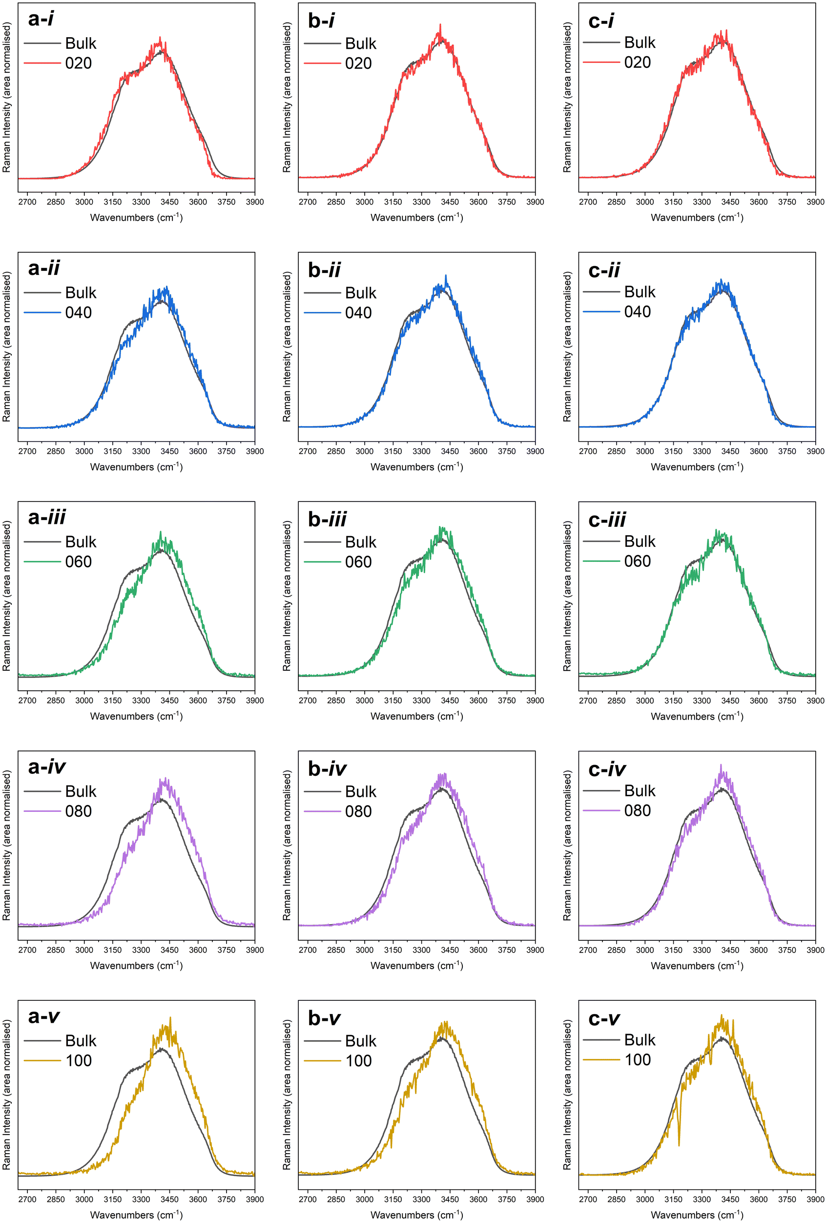

Fig. 1 Solute-correlated spectra presented alongside the bulk spectra for (i) 20%, (ii) 40%, (iii) 60%, (iv) 80%, and (v) 100% samples in the a. NP10, b. NP30 and c. NP50 series.

The spectral intensities at higher wavenumbers (higher energies) in the Raman O–H stretching signal are dominated by spectral contributions from water molecules having a smaller number of hydrogen-bonding possibilities fulfilled. Therefore, the gradual drop in spectral intensities in the lower wavenumber regions in all of the solute-correlated spectra, combined with a steady uptick in spectral intensities in higher wavenumber regions in them, with increasing Au NP concentration, indicates that the presence of the NPs in the dispersion results in a diminished extent of hydrogen-bonding in the surrounding water molecules.

For a purely qualitative assessment of the spectral differences, each of the bulk and solute-correlated spectra was fitted as a sum of three Gaussian functions (Fig. 2, with fitting parameters summarised in Table S3 in the ESI†). In the literature, Raman spectra of aqueous samples have often been fitted with five Gaussian peaks.^68–71 However, since only three peaks can be seen in water Raman spectra by visual inspection and keeping the number of peaks used to fit a curve to the minimum is an essential good practice in peak fitting,⁷² only three Gaussian fitting peaks were used in the current case. The first Gaussian fit peak (FP1) predominantly represents the Raman spectral contribution from fully hydrogen-bonded water. While the fitting is merely an approximate visualisation, it can still be consistently observed that in each of the fifteen instances explored, the area under the curve for the first Gaussian fit peak (FP1) does decrease (at the expense of an increase for the combined area of the two other fit peaks) in the solute-correlated spectrum compared to the share in the corresponding bulk spectrum (Fig. 3). The overall inference that can be drawn from the fitting is that the relative proportion of fully hydrogen-bonded water molecules (i.e., water molecules with four hydrogen-bonding interactions with neighbouring molecules) diminishes inside the hydration shell while the proportion of water molecules with a limited number of hydrogen-bonding interactions increases, compared with the bulk phase liquid. Therefore, the number of possible hydrogen-bonding interactions per molecule decreases on moving from the bulk to the hydration shell, on an average.

Fig. 2 Bulk and solute-correlated spectra for (i) 20%, (ii) 40%, (iii) 60%, (iv) 80%, and (v) 100% samples in the a. NP10, b. NP30 and c. NP50 series fitted with 3 Gaussian fitting components FP1, FP2 and FP3.

Fig. 3 Relative area under the curve (considering total area = 1) for Gaussian fitting components FP1, FP2 and FP3, plotted for a. NP10, b. NP30 and c. NP50.

The very distinctive decrease in the 3250 cm⁻¹ peak intensity in the solute-correlated spectra points towards the fact that the hydration shell molecules under consideration are further away (than their bulk phase counterparts) from meeting the perfect resonance conditions for the Fermi resonance between the fundamental O–H symmetric stretching mode and the first overtone of the H–O–H bending mode of vibration. This is likely to have been caused by a depletion in the number of hydrogen-bonding interactions per molecule in the hydration shell, compared to the number of such interactions possible in the bulk phase. The drop in the number of hydrogen-bonding interactions per molecule leaves the solvation shell with less means to support intermolecular coupling that would facilitate the Fermi resonance. This may present a contrasting image to that of water on the extended Au surface. The 3250 cm⁻¹ peak was reported to display stronger vibrational sum frequency generation intensity than the 3400 cm⁻¹ peak in water on the gold thin film,⁷³ which was understood as suggestive of a lack of disruption in the hydrogen-bonding network in the interfacial water on the extended gold surface. At the same time, further theoretical⁷⁴ and experimental⁷⁵ works report the greater relative population of dangling O–H at the gold/water interface, which suggests rupture of hydrogen-bonding interactions. Further clarity and reconciliation of these pictures can possibly be attained by gathering more spectroscopic evidence on interfacial water on an extended gold surface, which is in general experimentally challenging.⁷⁶

The apparent size-dependent variation of how stark the differences between the solute-correlated spectra and the bulk spectra are (Fig. 1) should be viewed with some caution. From Fig. 1, it is clear that the solvation shell around NP10 experiences the highest degree of disruption, followed by the solvation shell around NP30, while this disruption is the weakest in the case of NP50. This could potentially mean, among these three sizes of citrate-stabilised Au NPs, the 10 nm Au NPs have the greatest ability to rupture the water hydrogen-bonding network at the interfacial region, the 50 nm Au NPs have the lowest ability to cause the same while the 30 nm Au NPs fall in between the two in this regard. However, in this study, the crudely calculated surface area is the same only for NP30 and NP50. Also, the actual exposed surface area could be very different from the approximate surface areas calculated assuming perfect geometry. There could also be different degrees of defects on the surface that could alter the way water interacts with these NPs. These effects might be more pronounced in NPs of smaller sizes. Apart from that, the geometries, including shapes, of Au NPs can be intricately intertwined with their sizes.^77,78 Keeping these aspects in view, it is best only to take note of the apparent size-dependent variations of solute-correlated spectra and to use that as a starting point for a dedicated future study that aims to specifically control the mentioned parameters.

A dangling O–H peak at around 3700 cm⁻¹ clearly separated from the rest of the O–H band is observed in the spectra for water at hydrophobic interfaces.^20,79 No such separate dangling O–H peak can be observed in the solute-correlated spectra from the citrate-stabilised Au NPs (Fig. 1). This suggests the absence of water at the hydrophobic interface in the present system under study which goes along the line of the above-mentioned spectral similarities to polar and charged species. Apart from that, a slight blue shift in the position of maximum intensity is visible on moving from the bulk to solute-correlated spectra. However, in the crude spectral fitting, some solute-correlated spectra display a red shift for the peak at around 3250 cm⁻¹ (FP1 curves in Fig. 2), while others display a blue shift. One must stay cautious not to specifically pick up one fitted spectrum and exude confidence in attributing an inference with certainty to the corresponding sample. If a universal trend is observed, general inference can be drawn for all the samples, even from these approximate fittings. But in case a mixed trend is observed in these fitted spectra, conclusions about individual samples should not be drawn. That is because the exact numerical outputs can be dubious in these peak fittings due to the high overlap of the peaks coinciding with strong area variations. Therefore, the observation of blue or red shift in FP1 in a certain sample is not sufficient to assign an increase or decrease in the O–H bond strength of fully hydrogen-bonded water in that particular sample. However, speaking in general, the blue or red shifts in FP1 curves are both abundantly visible overall among the fifteen instances. Such an observation can possibly be attributed to the presence of interfacial water around the hydrophilic surface since the red or blue shift observed in vibrational frequencies of water at hydrophilic interfaces has been a controversial topic with conflicting reports and explanations.^19,67,80,81 After all, in the present case, a hydrophilic surface can be speculated to have been provided by the citrate coverage of Au NPs since negatively charged O-atoms (from citrate) should be able to participate in hydrogen bonding more efficiently than water O-atoms with a partial negative charge. Although the citrate concentrations used in all the samples are very low (always well below 1 mM, as per dilution factors in Table S1 and section 2 in the ESI†), the hydrophilic character of the solute correlated spectra pose the question whether the solute-correlated spectra primarily contain contributions of hydration shell water around citrate anions, and the presence of gold offers zero to minimal influence on the structure of hydration shell water around these nanoparticles.

Potential influence of citrate on interfacial water

To test for any influence of citrate on the observed solute correlated spectra of the studied Au NPs, Raman solute-correlated spectra of citrate at several concentrations were measured. As noted earlier, the citrate concentrations in the studied NP dispersions were well below 1 mM but the shape of the O–H stretching signal in the solute-correlated spectrum for 1 mM trisodium citrate dihydrate was already hardly distinguishable from that in the water Raman spectrum except for the faint appearance of the C–H stretching vibration bands around 2800–3000 cm⁻¹ (Fig. 4). This already demonstrates that the presence of such a low concentration of citrate in the NP dispersions could not have caused the extent of spectral variation between bulk and solute-correlated spectra observed in Fig. 1. Apart from that, it is noteworthy that the nature of variation in the spectral lineshapes caused by citrate is fundamentally different from the trends observed in Fig. 1. At higher citrate concentrations, solute-correlated spectra from the citrate solutions show a significantly reduced intensity at 3250 cm⁻¹ indicating a reduction of strongly hydrogen-bonded water in the solvation shell of citrate. In this particular aspect, the observed citrate solute-correlated spectra resemble the solute-correlated spectra of the Au NPs. However, in contrast to the Au NPs, the citrate solute-correlated spectra also show a significantly reduced intensity at 3610 cm⁻¹ indicating a loss in the relative population of very weakly hydrogen-bonded water molecules. The particular differences observed between the solute-correlated spectra of citrate and those of the Au NPs indicate that the structures of the solvation shells of both systems differ.

Fig. 4 The bulk and solute-correlated spectra for aqueous citrate solutions of a. 1 mM, b. 5 mM, c. 10 mM, d. 100 mM and e. 1000 mM strengths.

Nevertheless, citrate is known to adsorb to the Au NP surface, which is also supported by computational studies.⁵¹ Due to structural differences between adsorbed and fully solvated citrate ions, the conclusions drawn, firstly, from Fig. 4a and secondly, from the comparisons of the spectral lineshapes of the solute-correlated spectra in Fig. 1 and 4, are not sufficient to fully exclude the potentially major influence of citrate on the solute-correlated spectra of the Au NPs. Hence, to further ascertain the nature of the influence of citrate, MD simulations were performed.

It was found that Au(111) and sodium citrate both significantly perturbed the tetrahedral water structure, both independently and in tandem with each other. Examining these effects separately, the most significant perturbation was observed as a result of the Au(111) surface, depicted in Fig. 5. A significant and consistent perturbation was seen in this interfacial region, including in the absence of citrate (though strengthened with increasing citrate concentration).

Fig. 5 Distributions of the tetrahedral order parameter q, obtained from simulations a. in bulk phase and b. in the region close to the interface at various citrate concentrations.

The effect of the Au surface is observed as an increased number of water molecules with an intermediate tetrahedral order parameter of about 0.5 as opposed to a lower amount of highly ordered molecules (with q ≈ 0.8). This in itself is not surprising, as it has long been well understood that the structure of water is significantly perturbed in interfacial regions.^5,82 Whereas the effect of increasing citrate concentration in the bulk simulation results in a slight leftward shift in the distribution except at a very high concentration (500 mM), the effect from the interface results in a significant shift whereby the primary peak in the distribution is shifted by around −0.3 – a significant perturbation.

As noted, the effect of the citrate in the absence of the gold interface is significantly more limited than the impact of the interface. This may be in part due to the hydrophilicity of the citrate molecules as observed in the citrate–water RDFs (see Fig. S6†), whereby in particular, the 3 carboxylate groups engage in hydrogen bonding with water. However, the addition of citrate leads to a much more pronounced effect in tandem with the interface – leading to a much larger population of molecules with q ≪ 0.5. This indicates a much more significant disruption of the tetrahedral order and is likely enhanced by the higher effective concentration of citrate in the interfacial region due to the adsorption of both citrate and sodium to the gold surface.

It is thus clear that while the Au surface exerts a larger and more pronounced perturbation than citrate in isolation (as can be understood by comparing the grey curves in Fig. 5), the most significant effect comes from the citrate and Au surface exerting a combined influence on the water structure. It is also worth noting that the effect of the citrate in both cases also seems qualitatively similar, not changing the overall profile of the distribution curve but instead shifting it slightly leftwards.

It is important to note here while the shift in the tetrahedral order parameter indicates that the structure is perturbed from that expected of bulk water, it does not provide a full description of the exact structure, only that it is significantly less tetrahedrally ordered in particular. However, this outcome can logically be inferred to be a consequence of a loss in the population of fully hydrogen-bonded water molecules, as determined from the solute-correlated spectra in Fig. 1.

Conclusions

This work highlights the differences present in water molecules significantly perturbed by the presence of citrate-stabilised gold nanoparticles in an aqueous dispersion, when compared against bulk phase molecules further away from the nanoparticles. It could be inferred that the solvation shell has a diminished extent of hydrogen-bonding, which possibly comes along with a lower overall tetrahedrality, as suggested by modelling. This proposition fits well into the picture of a solvation shell comprised of less extensive intermolecular hydrogen-bonding, with fewer hydrogen-bonding possibilities per molecule, when compared with the bulk phase. Further experiments and MD simulations showed that the observed perturbations in the hydration shell water structure in the system under consideration can largely be attributed to the presence of gold nanoparticles and not primarily the citrate anions.

In future, it would be interesting to explore the similarities, or a lack thereof, between the structures of the hydrogen-bonding networks in water around the nanoscale as opposed to bulk Au samples, measured spectroscopically under comparable conditions. A dedicated study on the NP-size dependence of the scale of disruptions in the hydration shell hydrogen-bonding network could also be planned for the future by carefully controlling the surface features of the NPs.

Finally, this work has shown that Raman-MCR can be successfully implemented to study hydration shells of nanoparticles too. Therefore, Raman “solvation shell spectroscopy” can be expected to be useful in studying interfacial molecules around this class of solutes, like it has been for solutions of alcohol, ionic salts, etc.

Author contributions

Conceptualization and methodology: all authors; investigation, formal analysis, and visualization: TM (experiments and MCR) and ES (simulations); writing – original draft: TM (except simulations) and ES (simulations); writing – review & editing: MS and MR; funding acquisition, project administration, and supervision: MS (simulations) and MR (experiments and MCR).

Data availability

The raw Raman spectral datasets from the experiments referred to in this work are available at: https://doi.org/10.17617/3.JXONN3. All the details necessary to reproduce this work are available either in the article alongside its ESI† or on request from the corresponding authors.

Conflicts of interest

There are no conflicts to declare.

Acknowledgements

This work was funded by the Deutsche Forschungsgemeinschaft (DFG, German Research Foundation) under Germany's Excellence Strategy – EXC-2033–390677874 – RESOLV. TM thanks Prof. Poul Bering Petersen (Ruhr University Bochum) for providing an introduction to MCR. The authors thank the in-house workshop at MPI-SusMat for the preparation of the temperature regulation setup. Open Access funding provided by the Max Planck Society.

References

1. H. Erikson, G. Jürmann, A. Sarapuu, R. J. Potter and K. Tammeveski, Electrochim. Acta, 2009, 54, 7483–7489.
2. L. Wang, Z. Tang, W. Yan, H. Yang, Q. Wang and S. Chen, ACS Appl. Mater. Interfaces, 2016, 8, 20635–20641.
3. M. Gilles, E. Brun and C. Sicard-Roselli, J. Colloid Interface Sci., 2018, 525, 31–38.
4. J.-J. Velasco-Velez, C. H. Wu, T. A. Pascal, L. F. Wan, J. Guo, D. Prendergast and M. Salmeron, Science, 2014, 346, 831–834.
5. O. Björneholm, M. H. Hansen, A. Hodgson, L.-M. Liu, D. T. Limmer, A. Michaelides, P. Pedevilla, J. Rossmeisl, H. Shen, G. Tocci, E. Tyrode, M.-M. Walz, J. Werner and H. Bluhm, Chem. Rev., 2016, 116, 7698–7726.
6. M. Zobel, R. B. Neder and S. A. J. Kimber, Science, 2015, 347, 292–294.
7. R. Tandiana, E. Brun, C. Sicard-Roselli, D. Domin, N.-T. Van-Oanh and C. Clavaguéra, J. Chem. Phys., 2021, 154, 044706.
8. C.-H. Chan, F. Poignant, M. Beuve, E. Dumont and D. Loffreda, J. Phys. Chem. Lett., 2019, 10, 1092–1098.
9. R. S. Cataliotti, F. Aliotta and R. Ponterio, Phys. Chem. Chem. Phys., 2009, 11, 11258.
10. F. Novelli, M. B. Lopez, G. Schwaab, B. R. Cuenya and M. Havenith, J. Phys. Chem. B, 2019, 123, 6521–6528.
11. I. Hammami, N. M. Alabdallah, A. A. Jomaa and M. Kamoun, J. King Saud Univ., Sci., 2021, 33, 101560.
12. J. Turkevich, P. C. Stevenson and J. Hillier, Discuss. Faraday Soc., 1951, 11, 55.
13. T. Ishida, T. Murayama, A. Taketoshi and M. Haruta, Chem. Rev., 2020, 120, 464–525.
14. R. Fenger, E. Fertitta, H. Kirmse, A. F. Thünemann and K. Rademann, Phys. Chem. Chem. Phys., 2012, 14, 9343.
15. W. H. Lawton and E. A. Sylvestre, Technometrics, 1971, 13, 617–633.
16. A. de Juan and R. Tauler, Crit. Rev. Anal. Chem., 2006, 36, 163–176.
17. A. de Juan, J. Jaumot and R. Tauler, Anal. Methods, 2014, 6, 4964–4976.
18. D. Ben-Amotz, J. Am. Chem. Soc., 2019, 141, 10569–10580.
19. P. N. Perera, B. Browder and D. Ben-Amotz, J. Phys. Chem. B, 2009, 113, 1805–1809.
20. J. G. Davis, K. P. Gierszal, P. Wang and D. Ben-Amotz, Nature, 2012, 491, 582–585.
21. K. P. Gierszal, J. G. Davis, M. D. Hands, D. S. Wilcox, L. V. Slipchenko and D. Ben-Amotz, J. Phys. Chem. Lett., 2011, 2, 2930–2933.
22. A. A. Kananenka, N. J. Hestand and J. L. Skinner, J. Phys. Chem. B, 2019, 123, 5139–5146.
23. S. Saha, S. Roy, P. Mathi and J. A. Mondal, J. Phys. Chem. A, 2019, 123, 2924–2934.
24. M. Ahmed, V. Namboodiri, A. K. Singh, J. A. Mondal and S. K. Sarkar, J. Phys. Chem. B, 2013, 117, 16479–16485.
25. D. Zhou, L.-S. Wan, Z.-K. Xu and K. Mochizuki, J. Phys. Chem. B, 2021, 125, 12104–12109.
26. Y. Shen, B. Liu, J. Cui, J. Xiang, M. Liu, Y. Han and Y. Wang, J. Phys. Chem. Lett., 2020, 11, 7429–7437.
27. Y. Sun and P. B. Petersen, J. Phys. Chem. Lett., 2017, 8, 611–614.
28. A. Sokołowska and Z. Kecki, J. Raman Spectrosc., 1986, 17, 29–33.
29. G. E. Walrafen, J. Chem. Phys., 1966, 44, 1546–1558.
30. G. E. Walrafen, J. Chem. Phys., 1967, 47, 114–126.
31. G. E. Walrafen, M. R. Fisher, M. S. Hokmabadi and W.-H. Yang, J. Chem. Phys., 1986, 85, 6970–6982.
32. S. R. Pattenaude, L. M. Streacker and D. Ben-Amotz, J. Raman Spectrosc., 2018, 49, 1860–1866.
33. C. H. Camp, J. Res. Natl. Inst. Stand. Technol., 2019, 124, 124018.
34. K. R. Fega, A. S. Wilcox and D. Ben-Amotz, Appl. Spectrosc., 2012, 66, 282–288.
35. D. S. Wilcox, B. M. Rankin and D. Ben-Amotz, Faraday Discuss., 2013, 167, 177–190.
36. A. P. Thompson, H. M. Aktulga, R. Berger, D. S. Bolintineanu, W. M. Brown, P. S. Crozier, P. J. in ‘t Veld, A. Kohlmeyer, S. G. Moore, T. D. Nguyen, R. Shan, M. J. Stevens, J. Tranchida, C. Trott and S. J. Plimpton, Comput. Phys. Commun., 2022, 271, 108171.
37. A. S. Barnard, X. M. Lin and L. A. Curtiss, J. Phys. Chem. B, 2005, 109, 24465–24472.
38. Y. Xia, Y. Xiong, B. Lim and S. E. Skrabalak, Angew. Chem., Int. Ed., 2009, 48, 60–103.
39. A. S. Barnard, N. P. Young, A. I. Kirkland, M. A. Van Huis and H. Xu, ACS Nano, 2009, 3, 1431–1436.
40. H. Heinz, K. C. Jha, J. Luettmer-Strathmann, B. L. Farmer and R. R. Naik, J. R. Soc., Interface, 2010, 8, 220–232.
41. F. Iori, R. Di Felice, E. Molinari and S. Corni, J. Comput. Chem., 2009, 30, 1465–1476.
42. P. Drude, Ann. Phys., 1900, 306, 566–613.
43. I. L. Geada, H. Ramezani-Dakhel, T. Jamil, M. Sulpizi and H. Heinz, Nat. Commun., 2018, 9, 716.
44. R. Báez-Cruz, L. A. Baptista, S. Ntim, P. Manidurai, S. Espinoza, C. Ramanan, R. Cortes-Huerto and M. Sulpizi, J. Phys.: Condens. Matter, 2021, 33, 254005.
45. B. R. Brooks, C. L. Brooks III, A. D. Mackerell Jr., L. Nilsson, R. J. Petrella, B. Roux, Y. Won, G. Archontis, C. Bartels, S. Boresch, A. Caflisch, L. Caves, Q. Cui, A. R. Dinner, M. Feig, S. Fischer, J. Gao, M. Hodoscek, W. Im, K. Kuczera, T. Lazaridis, J. Ma, V. Ovchinnikov, E. Paci, R. W. Pastor, C. B. Post, J. Z. Pu, M. Schaefer, B. Tidor, R. M. Venable, H. L. Woodcock, X. Wu, W. Yang, D. M. York and M. Karplus, J. Comput. Chem., 2009, 30, 1545–1614.
46. L. B. Wright, P. M. Rodger and T. R. Walsh, RSC Adv., 2013, 3, 16399–16409.
47. R. Car and M. Parrinello, Phys. Rev. Lett., 1985, 55, 2471–2474.
48. P. Charchar, A. J. Christofferson, N. Todorova and I. Yarovsky, Small, 2016, 12, 2395–2418.
49. J. Zeng, S. Yang, H. Yu, Z. Xu, X. Quan and J. Zhou, Langmuir, 2021, 37, 3410–3419.
50. L. B. Wright, P. M. Rodger and T. R. Walsh, Langmuir, 2014, 30, 15171–15180.
51. O. A. Perfilieva, D. V. Pyshnyi and A. A. Lomzov, J. Chem. Theory Comput., 2019, 15, 1278–1292.
52. H. J. C. Berendsen, J. R. Grigera and T. P. Straatsma, J. Phys. Chem., 1987, 91, 6269–6271.
53. Y. Wu, H. L. Tepper and G. A. Voth, J. Chem. Phys., 2006, 124, 024503.
54. S. Izadi, R. Anandakrishnan and A. V. Onufriev, J. Phys. Chem. Lett., 2014, 5, 3863–3871.
55. A. Hjorth Larsen, J. Jørgen Mortensen, J. Blomqvist, I. E. Castelli, R. Christensen, M. Dułak, J. Friis, M. N. Groves, B. Hammer, C. Hargus, E. D. Hermes, P. C. Jennings, P. Bjerre Jensen, J. Kermode, J. R. Kitchin, E. Leonhard Kolsbjerg, J. Kubal, K. Kaasbjerg, S. Lysgaard, J. Bergmann Maronsson, T. Maxson, T. Olsen, L. Pastewka, A. Peterson, C. Rostgaard, J. Schiøtz, O. Schütt, M. Strange, K. S. Thygesen, T. Vegge, L. Vilhelmsen, M. Walter, Z. Zeng and K. W. Jacobsen, J. Phys.: Condens. Matter, 2017, 29, 273002.
56. E. Duboué-Dijon and D. Laage, J. Phys. Chem. B, 2015, 119, 8406–8418.
57. K. Ramasesha, L. D. Marco, A. Mandal and A. Tokmakoff, Nat. Chem., 2013, 5, 935–940.
58. D. M. Carey and G. M. Korenowski, J. Chem. Phys., 1998, 108, 2669–2675.
59. Q. Sun, Vib. Spectrosc., 2009, 51, 213–217.
60. Y. Harada, J. Miyawaki, H. Niwa, K. Yamazoe, L. G. M. Pettersson and A. Nilsson, J. Phys. Chem. Lett., 2017, 8, 5487–5491.
61. T. Morawietz, O. Marsalek, S. R. Pattenaude, L. M. Streacker, D. Ben-Amotz and T. E. Markland, J. Phys. Chem. Lett., 2018, 9, 851–857.
62. J. Wiafe-Akenten and R. Bansil, J. Chem. Phys., 1983, 78, 7132–7137.
63. D. E. Hare and C. M. Sorensen, J. Chem. Phys., 1992, 96, 13–22.
64. J. L. Green, A. R. Lacey and M. G. Sceats, J. Phys. Chem., 1986, 90, 3958–3964.
65. C. I. Ratcliffe and D. E. Irish, J. Phys. Chem., 1982, 86, 4897–4905.
66. S. Kint and J. R. Scherer, J. Chem. Phys., 1978, 69, 1429–1431.
67. P. Perera, M. Wyche, Y. Loethen and D. Ben-Amotz, J. Am. Chem. Soc., 2008, 130, 4576–4577.
68. R. Li, Z. Jiang, S. Shi and H. Yang, J. Mol. Struct., 2003, 645, 69–75.
69. R. Li, Z. Jiang, F. Chen, H. Yang and Y. Guan, J. Mol. Struct., 2004, 707, 83–88.
70. X. F. Huang, Q. Wang, X. X. Liu, S. H. Yang, C. X. Li, G. Sun, L. Q. Pan and K. Q. Lu, J. Phys. Chem. C, 2009, 113, 18768–18771.
71. A. J. Casella, T. G. Levitskaia, J. M. Peterson and S. A. Bryan, Anal. Chem., 2013, 85, 4120–4128.
72. R. J. Meier, Vib. Spectrosc., 2005, 39, 266–269.
73. S. M. Piontek, D. Naujoks, T. Tabassum, M. J. DelloStritto, M. Jaugstetter, P. Hosseini, M. Corva, A. Ludwig, K. Tschulik, M. L. Klein and P. B. Petersen, ACS Phys. Chem. Au, 2023, 3, 119–129.
74. A. Serva, M. Salanne, M. Havenith and S. Pezzotti, Proc. Natl. Acad. Sci. U. S. A., 2021, 118, e2023867118.
75. Y. Tong, F. Lapointe, M. Thämer, M. Wolf and R. K. Campen, Angew. Chem., Int. Ed., 2017, 56, 4211–4214.
76. E. H. G. Backus, N. Garcia-Araez, M. Bonn and H. J. Bakker, J. Phys. Chem. C, 2012, 116, 23351–23361.
77. X. Wei, B. Shao, Y. Zhou, Y. Li, C. Jin, J. Liu and W. Shen, Angew. Chem., Int. Ed., 2018, 57, 11289–11293.
78. B. Shao, J. Zhang, J. Huang, B. Qiao, Y. Su, S. Miao, Y. Zhou, D. Li, W. Huang and W. Shen, Small Methods, 2018, 2, 1800273.
79. L. F. Scatena, M. G. Brown and G. L. Richmond, Science, 2001, 292, 908–912.
80. H. Ratajczak, W. J. Orville-Thomas and C. N. R. Rao, Chem. Phys., 1976, 17, 197–216.
81. M. Rozenberg, A. Loewenschuss and Y. Marcus, Phys. Chem. Chem. Phys., 2000, 2, 2699–2702.
82. S. W. Devlin, F. Bernal, E. J. Riffe, K. R. Wilson and R. J. Saykally, Faraday Discuss., 2024, 249, 9–37.

---

Footnote

† Electronic supplementary information (ESI) available. See DOI: https://doi.org/10.1039/d5nr01153a

---