DOI:
10.1039/D5NR00602C
(Paper)
Nanoscale, 2025,
17, 12963-12980
Fast and accurate characterization of bioconjugated particles and solvent properties by a general nonlinear analytical relationship for the AC magnetic hysteresis area†
Received
10th February 2025
, Accepted 9th April 2025
First published on 29th April 2025
Abstract
Brownian magnetic nanoparticles present a large sensitivity to AC fields, opening new routes to bio-sensing using bio-functionalized nanoparticles. The integration of theory and experiment permits the transduction of any magnetic response (via susceptibility, harmonics or hysteresis area) to extract relevant system's parameters (such as particle size, solvent viscosity, and temperature). Parameter estimators based on linear response theory are easy to implement, but their sensitivity and resolution are limited by construction. Nonlinear responses allow for much higher sensitivities, but demand a significant cost in complex simulations to fit the experiments, because no analytical relationship is available. Here we have solved this dilemma by deriving an empirical analytical relationship for the magnetic hysteresis area which is valid under the arbitrary field intensity and frequency, thus avoiding the need for calibration. This universal relationship matches within 1% of the outcome of the nonlinear Fokker–Planck equation and has been validated against detailed Brownian dynamic simulations and controlled experiments. Using this nonlinear magnetic hysteresis area relationship, we have built an extremely fast automated searching algorithm that simultaneously estimates several system parameters by fitting experimental data for the area (at varying intensities and frequencies). The searching scheme starts with a robust and flexible stochastic method (parallel tempering Monte Carlo) followed by an accurate deterministic multi-variable minimization (Gauss–Newton) to match experimental areas within ∼1% deviation. This integrated approach upgrades AC-magnetometry into a stand-alone technique able to determine, with outstanding accuracy, particle size, polydispersity, concentration, and magnetic moment, as well as solvent viscosity and temperature. We validated this method in biosensing protocols by determining nanometer-size variations in bio-functionalized nanoparticles upon protein target recognition.
Introduction
The need for adaptable, accurate and sensitive diagnostic assays and biomarker detection tools has significantly increased in recent times. The key is to achieve a precise transduction of some measurable physicochemical signals into relevant biomolecular properties. Nanoparticles can now achieve this goal by placing specific receptors onto their surface to capture target biomolecules. The transduction mechanism should be thus highly dependent on their size, which will slightly increase upon any capture events. This makes the magnetic moment response dominated by Brownian rotational diffusion a perfect candidate for transduction. For any nanoscale phenomena, Brownian motion is the ultimate expression of the underlying molecular randomness. However, paradoxically, stochasticity expresses itself with an outstanding precision when the system is forced to respond to periodic oscillations. Although free diffusion is associated with dispersion, under oscillatory forcing, a phase shift between the force and the system response is created by diffusion or friction, which is the basis of many accurate techniques.1,2 Such an imperfect synchronization in energy transfer produces heat and a paradigmatic example is the AC magnetic hysteresis area observed when exposing magnetic nanoparticles (MNPs) to alternating magnetic fields (AMFs) (Fig. 1). The heat produced by lagging-behind oscillatory MNPs is the basis of hyperthermia applications, such as solid cancer treatments3–5 or heating mediators for drug delivery systems.6,7 Besides, since the last 20 years, MNPs have been also used in catalysis,8 environmental9 or biomedical applications,10 acting as imaging agents11–14 or transducers for biosensing technologies.15–22 The so-called Néel-type relaxation has so far attracted most of the investigations, particularly in hyperthermia applications.23 This relaxation mechanism is inherently magnetic as it involves thermal switching of the particle magnetic moment across its magnetic anisotropy axis, with average waiting times increasing exponentially with the anisotropy constant and the particle volume. In contrast, the relaxation of ferromagnetic MNPs (with blocked magnetic moment) is dominated by rotational diffusion. The angular diffusion of a particle of radius rh in a fluid with viscosity η and temperature T is half the inverse of a time, τB = 4πηrh3/(kBT), which involves both particle and medium properties. This fact is extremely useful for biosensing applications, as it could lead to accurate, multipurpose characterization tools. The idea is now recently receiving a great deal of attention22 with most methods based on the analysis of the complex magnetization signal details (the harmonics).24
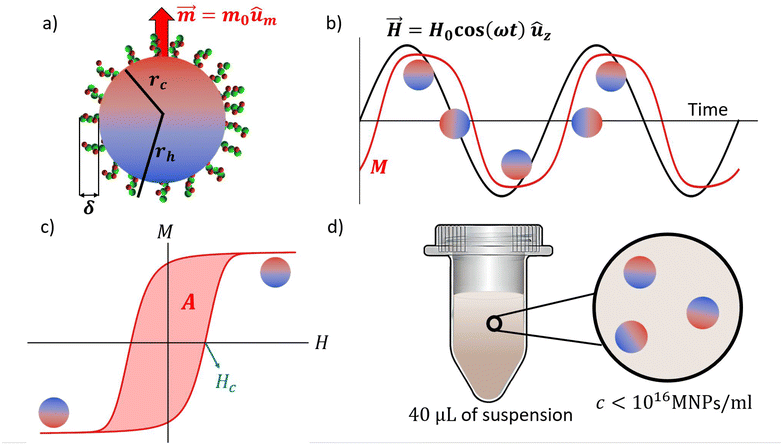 |
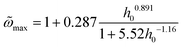
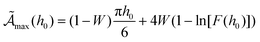
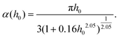
| | Fig. 1 (a) Schematic of the system under study, individual MNPs with the magnetic moment blocked that might be coated with some biomolecules. (b) Example of the variation of the magnetic field (black) and the magnetization of the system in the z direction (red) as a function of time for arbitrary parameters. (c) Example of an open hysteresis cycle in the magnetization field chart. The shadowed region is the area of the cycle and the coercive field is indicated in blue. (d) Schematic of the experimental system; 40 μL of a suspension of MNPs at a concentration such that dipolar interactions are negligible. | |
Here, we rather deployed the AC magnetic hysteresis area to prove and validate a method for fast and accurate characterization of particles and solvent properties. The motto driving the present theoretical and experimental efforts is the exceptional sensitivity of the MNP response under an AMF (in general) and its AC magnetic hysteresis area (in particular), which is able to detect few nanometer variations in the size of biofunctionalized particles upon protein capture.22 This great sensitivity has multiple origins. Rotational diffusion Dr = 1/(2τB) scales as the inverse particle volume rh−3, which is three times more sensitive to size (in relative variation d![[thin space (1/6-em)]](https://www.rsc.org/images/entities/char_2009.gif) lnDr/drh) than the translational one Dt ∼ rh−1 used by techniques such as dynamic light scattering (DLS)25 or nanoparticle tracking analysis (NTA).26 Moreover, AMF samples phase-lag at kHz rates, while DLS and NTA samples slow random motions and require very low concentrations,27,28 often overestimating the particle size.29 It comes as no surprise that our AMF-based measurements improve DLS and NTA measurements, both in accuracy and precision. This benefit is also present in other AMF-based techniques, notably in alternating current susceptometry (ACS) which is usually combined with the analytical relationships provided by linear response theory (LRT)15–17,30 (dating back to the Debye model31) to transduce AMF signals into particle sizes.32–38 However, ACS-LRT cannot benefit from two key properties offered by transducers working under non-linear response.20–22,39–41 First, while linear equations have a single solution and are fitted with a single parameter, non-linearity allows for multiple and simultaneous measurements (channels). Second, as we prove later on, the maximum area sensitivity against any system properties (again variation in the logarithm sense) is not located in the linear regime, but rather far from it. As a drawback, these “non-linear benefits” (multichannel fitting and higher sensitivity) demand paying a price in the computational cost, as closed relationships are simply not analytically derivable. For this task, solving Langevin dynamics for MNPs, which even allows for including dipolar and hydrodynamic interactions in dense suspensions,42,43 is simply too expensive to tackle the whole range of parameter space. In the context of parameter extraction, however, the controllable dilute regime is of primary interest and solving the (non-linear) Fokker–Planck equation (FPE) for the time-dependent MNP orientational distribution has been the common route,41,44–47 although other approximate alternatives exist.48 By expanding the sought distribution in an orthogonal functional basis, the FPE leads to an infinite hierarchy of ordinary differential equations (ODEs), which is truncated to achieve the desired precision.46 “Non-linear sensing” has been recently used by Yoshida et al.24 in a method which fits the experimental values of the magnetization harmonics series to simultaneously determine the distribution of the magnetic moment of MNPs, relaxation times and the particle concentration of even bimodal distributions. The proposed iterative method24 requires an accurate numerical solution of the FPE over each iteration and a rather complex algorithm to do it efficiently.
lnDr/drh) than the translational one Dt ∼ rh−1 used by techniques such as dynamic light scattering (DLS)25 or nanoparticle tracking analysis (NTA).26 Moreover, AMF samples phase-lag at kHz rates, while DLS and NTA samples slow random motions and require very low concentrations,27,28 often overestimating the particle size.29 It comes as no surprise that our AMF-based measurements improve DLS and NTA measurements, both in accuracy and precision. This benefit is also present in other AMF-based techniques, notably in alternating current susceptometry (ACS) which is usually combined with the analytical relationships provided by linear response theory (LRT)15–17,30 (dating back to the Debye model31) to transduce AMF signals into particle sizes.32–38 However, ACS-LRT cannot benefit from two key properties offered by transducers working under non-linear response.20–22,39–41 First, while linear equations have a single solution and are fitted with a single parameter, non-linearity allows for multiple and simultaneous measurements (channels). Second, as we prove later on, the maximum area sensitivity against any system properties (again variation in the logarithm sense) is not located in the linear regime, but rather far from it. As a drawback, these “non-linear benefits” (multichannel fitting and higher sensitivity) demand paying a price in the computational cost, as closed relationships are simply not analytically derivable. For this task, solving Langevin dynamics for MNPs, which even allows for including dipolar and hydrodynamic interactions in dense suspensions,42,43 is simply too expensive to tackle the whole range of parameter space. In the context of parameter extraction, however, the controllable dilute regime is of primary interest and solving the (non-linear) Fokker–Planck equation (FPE) for the time-dependent MNP orientational distribution has been the common route,41,44–47 although other approximate alternatives exist.48 By expanding the sought distribution in an orthogonal functional basis, the FPE leads to an infinite hierarchy of ordinary differential equations (ODEs), which is truncated to achieve the desired precision.46 “Non-linear sensing” has been recently used by Yoshida et al.24 in a method which fits the experimental values of the magnetization harmonics series to simultaneously determine the distribution of the magnetic moment of MNPs, relaxation times and the particle concentration of even bimodal distributions. The proposed iterative method24 requires an accurate numerical solution of the FPE over each iteration and a rather complex algorithm to do it efficiently.
Phenomenological relationships circumvent the need for costly FPE numerical solvers and substantially reduce the fitting effort. They are applied to determine experimentally accessible quantities and have proven to be highly effective in measuring solution viscosities,49 fluid temperature,50,51 simultaneous viscosity and temperature,52 and even temperature and particle size.53 However, their validity is typically limited to specific parameter ranges and require prior calibration with a well-known system before they can be used to determine other quantities. This limitation certainly constrains their predictive capacity.
In this work, we propose an optimal combination of both approaches. First, we numerically solved the FPE over the whole range of governing parameters, and then we integrated all this information into an analytical phenomenological relationship for the AC magnetic hysteresis area which is universal in the sense it is valid for any combination of external parameters (frequency f and field intensity H0). Instead of fitting a broad range of magnetic parameters, such as the amplitude and phase of multiple harmonics,21 a key point to achieve our goal in efficiency is to restrict our analysis to the AC magnetic hysteresis area, which is the only fitted parameter used to extract system's properties from a series of signals at varying f and H0 values. The protocol for parameter estimation is based on an efficient combination of parallel-tempering Monte Carlo followed by second-order accurate Gauss–Newton methods. We first validated its accuracy and precision using signals from accurate Langevin dynamics simulations. Then we applied it to experiments with uncoated MNPs, measuring their size and magnetization as well as the viscosity of several embedding solvents (glycerol–water mixtures). In more stringent biosensing tests, we determined nanometer variations in size of MNPs coated with dextran, then conjugated with proteins and finally after biomolecular recognition with target biomolecules. Our estimates for particle size distributions are compared with NTA and DLS and with the much more “exact” transmission electron microscopy (TEM); the magnetization of particles was compared with a superconducting quantum interference device (SQUID) and we estimated solvent viscosities with an outstanding agreement with standard rheometers. The results are in perfect agreement with TEM and SQUID and improve the precision and accuracy of NTA and DLS size estimation. As a relevant conclusion, we highlight that the present theoretical–experimental integrated approach upgrades AC-magnetometry as a stand-alone experimental device able to determine a significant list of properties of both solvents and particles, being of particular relevance for biosensing.
Universal relationship for the magnetic hysteresis area
We consider a number  of suspended magnetic nanoparticles (MNPs) in a volume
  (concentration
  ). The magnetic moment of each MNP is m0 and the saturation magnetization Ms = m0/[(4/3)πrc3] is determined by their magnetic core radius rc. In general, MNPs may present a coating layer of thickness δ, such that their hydrodynamic radius is rh = rc + δ. The solution was exposed to an AC magnetic field H(t) oscillating in the z direction at an angular frequency of ω = 2πf. The delay in the system's magnetization M(t) with respect to H(t) leads to some heat dissipated per cycle, equal to the area
  enclosed in the H–M chart (Fig. 1c). In deriving a general relationship for this magnetic hysteresis area, it is convenient to reduce the number of free parameters by working with non-dimensional variables. The non-dimensional area, defined as
  , only depends on the dimensionless frequency
  and the field amplitude h0 = μ0m0H0/kBT. Here μ0 is the magnetic permeability of vacuum and we recall the Brownian rotational relaxation time τB = 4πηrh3/(kBT). To extract the general relationship
  , we have solved the Fokker–Planck equation for the time-dependent probability distribution of the magnetization of a single particle (see the Materials and methods section). This approach is valid for dilute suspensions of MNPs that relax predominantly via the Brownian mechanism, as in such a case the total magnetization is simply proportional to the single-particle magnetization and the phenomena related to Néel relaxation, including anisotropy barrier crossings, are negligible. The limit of validity of the dilute regime can be estimated from the strength of particle–particle interactions‡ leading to c < 1016 MNPs per mL (or c < 15 μM). We note that these are not actually “extremely dilute” concentrations by experimental standards: experiments presented hereafter were conducted for c ≈ 5 × 10¹³ MNPs per mL, thus well within the dilute limit.
On the other hand, it is well known that the dominant relaxation mechanism depends on the applied magnetic field. Specifically, when the amplitude of the AMF is sufficiently high for the magnetic moment of the particles to overcome the anisotropy barrier, the Néel mechanism may become dominant. This imposes an upper limit on the values of h0 for which the phenomenological equation remains valid. This limit is determined by the condition Uext > Uanis, where the energy of the particles under an external field is given by Uext = μ0H0MsVc, and the energy required to cross the anisotropy barrier is Uanis = KVc. This leads to an inequality H0 < K/(μ0Ms). For cobalt ferrite nanoparticles, which typically have an anisotropy constant of K ≈ 105 J m−3 and a saturation magnetization of Ms = 2 × 10⁵ A m−1, this results in a maximum magnetic field amplitude of approximately 400 kA m−1. This value is significantly higher than the magnetic fields used in this study and those achievable in most experimental setups.
We performed an extensive set of calculations using the FPE equation to calculate  over a wide range of values of
  and h0. The analysis of this extensive information leads us to derive an accurate empirical relationship for
  . This useful “universal” magnetic area empirical relationship is one of the important results of this work,
| |  | (1) |
with
| |  | (2) |
and
| | | p0 = 1 − 0.45exp[−8.5h0−1.75] | (3) |
| |  | (4) |
| |  | (5) |
| |  | (7) |
Note that  in eqn (2) corresponds to the frequency maximizing the area for a fixed intensity h0. In other words,
  is the maximum area obtained at h0, given by:
| |  | (8) |
where
W = exp[−0.5
h0−1.8] acts as a weighting function that governs the transition between the linear (
W ≈ 0) and nonlinear (
W ≈ 1) regimes and
| F(h0) = 1 + 0.3h00.9 + 0.056h01.65 + 1.54 × 10⁻⁵h03.21. |
We shall soon show that this maximum in the area (i.e., in dissipated heat) takes place at the transition from the linear response (Debye model) to the non-linear regime. The coefficients ci in eqn (1) are finally given by:
| |  | (9) |
| |  | (10) |
| |  | (11) |
| |  | (12) |
with
| |  | (13) |
To illustrate the accuracy of eqn (1), Fig. 2a compares the area obtained from the solution of the FPE  with
with  for h0 = 1, 10, 100, and 1000 and a broad range of
  values. Differences between
  (symbols) and
  (lines) are not observable with the naked eye. For more precision in the deviation, panel (b) presents a contour plot of the relative error between the FPE and eqn (1) spanning five orders of magnitude in both
  and h0 (0.01 ≤ h0 ≤ 1000). Remarkably, the relative error remains always below 1.5%. We provided a first test for this “universal area relationship” against experiments in Fig. 2c and d where we compared eqn (1) with values of the AC magnetic hysteresis area created using cobalt ferrite MNPs (dominated by Brownian relaxation). Measurements were conducted for frequencies in the range of 10–100 kHz and using several solvents, whose viscosities were modified by adding glycerol in water up to a volumetric percentage of 45%. This experimental test also illustrates the utility of deploying non-dimensional variables to gather results from quite different parameters in single master curves. Values of these non-dimensional parameters (
 , h0 and
  ) were obtained by taking the liquid mixture viscosity from ref. 54 (Table 3) and the hydrodynamic radius of MNPs provided by TEM (this approximation is valid since the particles are quasi-spherical and lack any surface coating). The experimental measurements in Fig. 2c and d show an excellent agreement with
  in eqn (1), confirming it usability for parameter estimation in experiments.
 |
| | Fig. 2 (a) Comparison between the dimensionless magnetic area evaluated from the numerical solution of the Fokker–Planck equation (FPE) (dots) and the outcome of the empirical relationship in eqn (1) (lines) as a function of  for different values of h0. (b) Contour plot of the relative area difference between the FPE and eqn (1). (c and d) Comparison between the experimental values of the area as a function of the dimensionless frequency for different values of h0. (b) Contour plot of the relative area difference between the FPE and eqn (1). (c and d) Comparison between the experimental values of the area as a function of the dimensionless frequency  and the predictions of eqn (1) measured for field frequencies ranging from 10 kHz to 100 kHz and various glycerol concentrations, which alter the viscosity of the solution, for two field intensities: (c) 4 kA m−1 and (d) 24 kA m−1. For the calculations, particles were modeled with a log–normal size distribution with a mean radius of rc = rh = 13.6 nm, a standard deviation of σc = 1.3 nm, and a saturation magnetization of Ms = 179 kA m−1. and the predictions of eqn (1) measured for field frequencies ranging from 10 kHz to 100 kHz and various glycerol concentrations, which alter the viscosity of the solution, for two field intensities: (c) 4 kA m−1 and (d) 24 kA m−1. For the calculations, particles were modeled with a log–normal size distribution with a mean radius of rc = rh = 13.6 nm, a standard deviation of σc = 1.3 nm, and a saturation magnetization of Ms = 179 kA m−1. | |
Asymptotic regimes
We now analyze the different magnetization regimes and the different scaling laws for the magnetic area. Fig. 3a presents the contour plot of  from the numerical solution of the FPE. The plot reveals different regimes with distinct area scaling separated by a central region in the
  chart, where
  is maximum (see also Fig. 2a, c and d).
 |
| | Fig. 3 (a) Two-dimensional colormap depicting the variation of  as a function of the dimensionless parameters as a function of the dimensionless parameters  and h0 obtained by numerically solving the FPE. The black dashed line represents the value of and h0 obtained by numerically solving the FPE. The black dashed line represents the value of  that maximizes the area for each h0. (b) Two-dimensional colormap illustrating the relative error between the area predicted by LRT and the area obtained from the FPE as a function of the dimensionless parameters. The black dashed line highlights the isocontour where the relative error reaches 1%. (c) Maximum cycle area as a function of h0. The green line represents the theoretical upper bound, the red line corresponds to the LRT prediction, and the orange line depicts the prediction from eqn (8). (d) Value of that maximizes the area for each h0. (b) Two-dimensional colormap illustrating the relative error between the area predicted by LRT and the area obtained from the FPE as a function of the dimensionless parameters. The black dashed line highlights the isocontour where the relative error reaches 1%. (c) Maximum cycle area as a function of h0. The green line represents the theoretical upper bound, the red line corresponds to the LRT prediction, and the orange line depicts the prediction from eqn (8). (d) Value of  that maximizes the area as a function of h0. The red line shows the LRT prediction, the green line represents the asymptotic scaling that maximizes the area as a function of h0. The red line shows the LRT prediction, the green line represents the asymptotic scaling  , and the orange line corresponds to eqn (2). , and the orange line corresponds to eqn (2). | |
We start by stating that relationship 1 correctly recovers the linear response theory (LRT) result:
| |  | (14) |
The validity of the LRT or Debye model result (small h0 or large  ) is clearly deduced from Fig. 3b, showing the relative error of the LRT
  (see also Fig. 3d). In terms of non-dimensional quantities, the validity domain of the LRT turns out to be extremely simple: h0 ≲ 0.4 for any
  and the region
  . From the definitions given above, one realizes that the
  group represents the ratio between the energy provided by the external field to the magnet and the energy dissipated by the viscous torque. Hence, the LRT works when the viscous energy dissipation is faster than the external power reaching the magnet. In passing, the color scales of Fig. 3a and c indicate that the nondimensional area is bounded such that
  . Indeed, it is constrained by the rectangle defined by the x-bounds |h(t)/h0| < 1 and the y-bounds |
![[M with combining tilde]](https://www.rsc.org/images/entities/i_char_004d_0303.gif) (t)| ≤ 1, where
(t)| ≤ 1, where  and h(t) ≡ μ0m0H(t)/kBT. Note that such a constraint in the non-dimensional area is clearly not satisfied by the linear approximation in eqn (14).
We now consider the different asymptotic regimes observed as one varies the field intensity h0. At low field amplitudes (h0 < 1), the thermal energy surpasses the magnetic energy, leading to a predominantly randomized orientation of the magnetic moments. As a result, the system exhibits negligible average magnetization and an almost imperceptible hysteresis loop area. This region (small h0) roughly corresponds to the regime where LRT is valid, predicting a linear increase in  with h0 (as shown in eqn (14)). As h0 increases (with
  held constant), the area
  reaches a peak before decreasing again at higher field amplitudes. This behaviour represents a genuine non-linear effect, not captured by the LRT (see Fig. 4a illustrating the H–M chart and the ESI† for more details). On further increasing h0, the magnetic moments tend to remain aligned with the field direction for most of the cycles, entering the saturation regime. Only when the applied field approaches the coercitivity value Hc (Fig. 1c) do the moments quickly reorient. Consequently, the hysteresis loop shrinks as h0 increases further, as shown in Fig. 4a and c. In this high intensity h0 regime, the area scales as:
| |  | (15) |
 |
| | Fig. 4 (a and b) Hysteresis loops plotted in terms of the scaled field h(t)/h0 and the dimensionless magnetization . In panel (a),  and h0 varies with high values. In panel (b), h0 = 25 is fixed and the loops are computed for various values of and h0 varies with high values. In panel (b), h0 = 25 is fixed and the loops are computed for various values of  . The static response described by the Langevin equation L(h) is shown as a black line. (c) Variation of the AC magnetic hysteresis area with h0 for large values and different values of . The static response described by the Langevin equation L(h) is shown as a black line. (c) Variation of the AC magnetic hysteresis area with h0 for large values and different values of  . (d) AC magnetic hysteresis area as a function of . (d) AC magnetic hysteresis area as a function of  in the low-frequency regime in the low-frequency regime  for various values of h0. In panels (c) and (d), the dots indicate the results obtained by solving the FPE and the lines indicate the predictions of eqn (15) and (16), respectively. for various values of h0. In panels (c) and (d), the dots indicate the results obtained by solving the FPE and the lines indicate the predictions of eqn (15) and (16), respectively. | |
Concerning the frequency response (Fig. 4b and d), the AC magnetic hysteresis area is small at low frequencies  because the magnetization efficiently responds to the time variation of the applied field; in the limit
  , the hysteresis vanishes and the system magnetization M follows the static behavior described by the Langevin function (Fig. 4b, black line). High intensity h0 > 1 and low frequency
  are well outside the LRT. Fig. 4d shows the scaling law for the area in this region, which follows as:
| |  | (16) |
where
α(
h0) is given in
eqn (13) and for small
h0, it converges to
αLRT(
h0) = π
h0/3. Finally, in the high-frequency regime,

, the external field oscillates faster than the magnetic relaxation time,
τB, and the magnetic moments can no longer follow the rapidly changing field. This leads to a smaller magnetization and a reduced AC magnetic hysteresis area. At low field values
h0 < 1 the maximum area takes place for

. This result is consistent with a sort of stochastic resonance correctly captured by LRT (
eqn (14)), which predicts more dissipation when the relaxation rate 1/
τB coincides with
ω. However, the non-linear response to high external fields alters the location of the maximum dissipation towards larger frequencies

, as shown in
Fig. 3a and d (black dashed line). The LRT also severely fails in this regime as its maximum area increases without bounds with
h0, as

. However, as previously noted (
Fig. 4b and
3c), the maximum value of the non-dimensional area is capped at

and this limit is reached for
h0 → ∞ following a logarithmic trend. The agreement between

in
eqn (8) and the FPE's maximum area is perfect, as shown in
Fig. 3c.
Simultaneous determination of system's properties by cost-error minimization
The excellent accuracy of the universal empirical relationship for the magnetic hysteresis area (eqn (1)) opens a route to a fast determination of the multiple systems’ properties controlling the area. The experimental setup imposes the magnetic field amplitude H0 and frequency f that, in non-dimensional form, are noted as  . The collection of unknown “fundamental system's variables” is notated as
  and contains the hydrodynamic radius and magnetic moment of MNPs, the solvent viscosity, and the temperature and number of MNPs. Yet, in many practical applications, these properties,
  , are not single-valued but rather follow a distribution. We will characterize the first two moments of such distributions pi(λi): the mean 〈λi〉 and the variance σλi2. The shape of these marginal distributions pi(λi) such that p(λ) = Πipi(λi) are part of the model: typically we used a delta for single-valued variables, a Gaussian or a log–normal distribution depending on the specific variable (see the Materials and methods section). This leads to a generalization of the vector of unknown variables, which is noted as Λ = {〈λ〉, σλ}. The “theoretical” average area in dimensional units was obtained from relationship 1 weighted by p(λ; Λ) as:
| |  | (17) |
where we recall that h0 depends on the vector of parameters λvia m0 and T. Our target is to evaluate the value Λ = Λ* that minimizes the difference between the experimental area Aexp(Λ*) and the “theoretical” expression given by eqn (17). To this end, we have developed a “parameter estimator” that finds Λ*, minimizing a cost-error function  given by:
| |  | (18) |
Importantly, the sum in eqn (18) runs over a number of independent experimental measurements Nex (typically between 8 and 24) under varying frequencies and field-intensities: ξ(i) with i∈[1, Nex]. The searching protocol combines an initial stochastic search in the parameter space (parallel tempering Monte Carlo), followed by an accurate deterministic minimization (second-order Gauss–Newton scheme). Both steps are detailed in the Materials and methods section. The parallel tempering Monte Carlo (MC)55 is able to locate the minima under quite general starting conditions in the parameter space. Once the cost function levels below the chosen threshold, the scheme uses the second order Gauss–Newton (GN) algorithm to refine the solution. The resulting fitting protocol is quite fast and we made it available in the repository.56 It is implemented in C++, with Python bindings for easy usage.
To validate the protocol, we now assess its precision by comparing with numerical simulations with exactly known system parameters. In the next section, we used the parameter estimator to determine experimental data related to MNPs and the solution viscosity.
Assessing the accuracy in the parameter estimation from numerical simulations
In order to validate the fitting methodology and estimate its accuracy, we performed Brownian dynamics (BD) simulations22 of MNPs under an AC field. The magnetic radius rc and coating thickness δ used in the BD runs were chosen to closely match the experimental values (see below). Additionally, consistent with the typical distribution of nanoparticle sizes,57 we sampled rc values from a log–normal distribution with a mean rc = 15 nm and varying polydispersities (standard deviations σc/rc∈[0.1, 0.5]). We explored several coating thicknesses δ∈[0, 12.5] nm and a saturation magnetization of Ms = 150 kA m−1. In this test, Aexp corresponds to the results from BD simulations. As noted above, the cost function is based on a set of Nex experiments consisting of frequency dependence studies of the AC magnetization cycles (see the Materials and methods section) at different field intensities (4, 12 and 24 kA m−1), leading to a total of Nex = 24 cases, which are fitted simultaneously. This set of conditions mirrors those used in the experiments.
It is important to note that the accuracy of the Λ* prediction tends to decrease as the number of experiments used in the fits is reduced. As shown in the ESI,† achieving a reliable estimation of the parameters requires the utilization at least two different field intensities and 4–5 frequency values.
To optimize any fitting procedure, it is important to restrict the unknown parameters. However, as a first stringent test, we set δ = 0 (i.e., no coating, so the hydrodynamic and magnetic radii coincide, rh = rc) and assumed that Ms is the same in all the particles, so m0 = (4/3)πMsrc3. Under these assumptions, we simultaneously estimated the average core radius 〈rc〉, the standard deviation of distribution σc, the number of particles in the suspension, and the saturation magnetization Ms for different values of σc.
The results summarized in Table 1 indicate that the estimated values for Ms, rc, σc, and  closely match the “true” values used in the BD simulations. In all instances, the relative error remains consistently of the order of 1% or smaller for each parameter, highlighting the method's high accuracy in determining unknown system parameters.
Table 1 Parameters of MNPs determined by applying the present method to BD simulations, in which Ms = 150 kA m−1, rc = 15 nm,  , and σc takes various values that are indicated in the first column
| Simulations |
Present method |
|
σ
c/rc |
σ
c/rc |
r
c (nm) |
M
s (kA m−1) |

|
| 0.1 |
0.099 ± 0.006 |
15.0 ± 0.1 |
150.5 ± 0.6 |
(0.998 ± 0.005) × 105 |
| 0.25 |
0.241 ± 0.008 |
15.2 ± 0.2 |
150.3 ± 0.2 |
(0.992 ± 0.002) × 105 |
| 0.5 |
0.500 ± 0.005 |
14.9 ± 0.1 |
149.3 ± 0.2 |
(1.000 ± 0.001) × 105 |
In a second test, we evaluated the ability of the parameter estimator to quantify variations in hydrodynamic size when a coating is added to the particles. Following the experimental approach, we assumed that the bare MNPs had already been characterized, with rc, Ms, and σc known as fixed parameters. Thus, the goal was to determine the hydrodynamic radius of the particles (rh = rc + δ) by sampling over δ. We studied five different cases with increasing values of δ. The results, shown in Fig. 5a, demonstrate that this method can accurately determine the hydrodynamic size of the particles. In particular, an analysis of the relative error between the fitted hydrodynamic radius and the value used in the simulations (Fig. 5b) reveals that the error is consistently below 0.15%. Fig. 5c and d present the dependence of the relative error in the estimated system's parameters with the number of area measurements Nex. Notably, about Nex = 10 area measurements (at different fields and frequencies) are enough to obtain relative errors of about 10−2 in the magnetic saturation Msat and the average particle radius rc. The dispersion in size distribution σc requires about 20 measurements to yield such one percent error. Notably, the errors decrease down to the 0.1% range for Nex ∼25, which is the suggested value.
 |
| | Fig. 5 (a) Hydrodynamic radii of the MNPs for various coating widths determined using the fitting algorithm (red dots) compared with the values used in the simulations (black line). (b) Relative error between the expected hydrodynamic radius and the values obtained from the fitting. (c and d) Relative error between the estimated parameters and the values used in the BD simulations (Ms = 150 kA m−1, rc = 15 nm, and σc = 0.1rc) as a function of Nex. Panel (c) shows the results for Ms, while panel (d) presents the results for rc (green) and σc (purple), corresponding to the average particle size and the standard deviation, respectively. The results correspond to the datasets with three field intensities: H0 = 4, 12, and 24 kA m−1 and varying numbers of field frequencies (see the additional data in the ESI†). | |
Determining system's properties from experiments
Next, we applied the same methodology to determine multiple experimental parameters in different situations. In all experiments, we used cobalt ferrite nanoflowers. First, we employed uncoated (“plain”) p-MNPs with –COOH groups on their surface to provide colloidal stability. From the measurements of the cycle areas, we determined their saturation magnetization, the distribution of crystal sizes and the concentration of particles.
Once these particles have been characterized, we used them to determine the viscosity of glycerol solutions at different concentrations. Finally, we used the same method to study how the hydrodynamic size of the particles changes when a dextran coating is added and they are functionalized with ligands that interact with other biomolecules in the solution.
Determination of the core radius and magnetic moment of p-MNPs
To demonstrate the potential of the method for determining the crystal size and magnetic moment of MNPs, we analyzed raw experimental data on the AC magnetic hysteresis area of p-MNPs. Using our parameter estimator, we determined the core size and magnetic moment of bare MNPs. To validate these predictions, we compared them with TEM, NTA, and DLS measurements for particle size and SQUID measurements for magnetic moment. The experimental results of the area against the frequency are shown in Fig. 6a, in which the circles indicate experimental values and the lines indicate eqn (1) using the best parameter estimation (obviously δ = 0 was fixed). The comparison between the values of our parameter estimator and the experimental ones can be found in Table 2.
 |
| | Fig. 6 AC magnetic hysteresis area as a function of field frequency for three different field amplitudes: 4 kA m−1 (red), 12 kA m−1 (blue), and 24 kA m−1 (green) measured for water–glycerol mixtures at various glycerol concentrations: (a) 0% by volume, (b) 15%, (c) 32%, and (d) 45%. The dots represent experimental data, while the solid lines correspond to the fits obtained using the presented algorithm. | |
Table 2 Mean hydrodynamic radius (rh) obtained using the present method compared with the reported values through different methods in ref. 58
| Present method |
TEM |
DLS |
NTA |
| 13.6 ± 0.2 nm |
13.58 nm |
15 nm |
∼20 nm |
There is a perfect agreement between the present method and the sizes determined from TEM images (ESI†), which is the most reliable and exact size-measurement device. DLS slightly overestimates the hydrodynamic size but the agreement is also very good. Finally, NTA presents a much larger inaccurate value because our particles are below the NTA limit of detection (∼20 nm) which significantly biases the measure towards the largest particles of the ensemble. TEM images (ESI†) also provide the standard deviation in size, σc = 1.6 nm, which agrees with our estimation σc = (2.4 ± 0.2) nm extracted by assuming a log–normal distribution for rc into the fitting protocol (see the Materials and methods section). The size standard deviation is slightly overestimated by our method, which might be a consequence of the dispersion in Ms amongst the particles due to variations in the relative orientation of the different coalescent cores forming these particles. In any case, the fitted value of the effective saturation magnetization is Ms = 166.5 ± 0.2 kA m−1, which is also in close agreement with the value obtained using SQUID measurements, Ms = 179 kA m−1. The estimated number of particles in the suspension was 2.12 × 10¹², which for the volume employed in the experiments 40 μL corresponds to a concentration of 5.3 × 10¹³ MNP per ml (or ∼80 nm). This value is in agreement with the concentration of ∼3 × 10¹³ MNP per ml estimated from the experimental mass density 1 gFe+Co L−1 of roughly spherical particles with a radius of 13.6 nm and a density of ∼5.25 g cm−3. Possible differences between both estimations arise because particles are not perfect spheres but nanoflowers (ESI†), so their volume is smaller than the spherical estimation.
Determination of the viscosity of glycerol solutions at different concentrations
To demonstrate the capability of the fitting algorithm to determine the solution viscosity, we revisited the experimental data in Fig. 2c and d corresponding to a set of samples with varying viscosities obtained from mixtures of glycerol and water at different volume percentages (see the Materials and methods section). In this case, we left the viscosity as the only free parameter in the fitting scheme and self-consistently deployed the protocol as a viscosimeter. We performed measurements for glycerol solutions in water with glycerol of 0%, 15%, 32%, and 45% in volume. For each concentration, we measured the AC magnetization cycles at different field frequencies and at three field intensities (H0 = 4, 12, and 24 kA m−1). The viscosity is taken as the sole free parameter in the fits and, to use a self-consistent approach, the size of MNPs is first characterized by the fitting protocol in pure water (i.e., 0% glycerol). The results are summarized in Table 3, along with the viscosities based on the empirical formula presented in ref. 54. We observed almost perfect agreement between our results and the expected values, confirming that this method is highly effective as a viscosimeter.
Table 3 Comparison between the literature values of the viscosity of different mixtures of glycerol concentration and water at 25 °C and the measured value using the presented algorithm
| Glycerol concentration (%volume) |
Fitted viscosity (mPa s) |
Literature viscosity (mPa s) |
| 0 |
0.871 |
0.893 |
| 15 |
1.450 |
1.444 |
| 32 |
2.80 |
2.80 |
| 45 |
5.134 |
5.22 |
To further reinforce the protocol, in Fig. 6, we compared the experimental results of the area with the fits for all the measurements, showing that the values obtained through the fitting algorithm reproduce the experimental ones almost exactly.
Determination of the hydrodynamic radius of coated MNPs with different molecules on their surface
To highlight the potential of the method to analyze more complex scenarios, we applied our fitting algorithm to study variations in the hydrodynamic size of the particles when their surface is modified by changing the attached molecules. Specifically, the four types of surfaces studied are summarized in the insets of panels (a)–(d) in Fig. 7: panel (a) shows the previously studied p-MNPs; panel (b) depicts cobalt ferrite MNPs coated with dextran (D-MNPs); panel (c) represents MNPs bioconjugated with receptors (f-D-MNPs); and panel (d) illustrates f-D-MNPs after being immersed in a 2 μM solution and allowed to reach chemical equilibrium. The experimental values of the hysteresis areas under different field conditions (blue and red symbols in Fig. 7), as well as the mean hydrodynamic radius obtained through NTA measurements of the translational diffusion coefficient, are taken from ref. 22 and 58. The magnetic properties of the particles, such as Ms, rc, and σc, may slightly differ from previously measured values due to batch-to-batch variations in synthesis. These differences can lead to slight changes in core size and the dextran coating may prevent surface oxidation, potentially altering the Ms value.59 Situations where initial knowledge of certain parameters is partial or inaccurate are common; however, the flexibility of the MC scheme allows for easy adaptation. We employed a modified cost function with a soft bias toward the available initial information:  , where the parameters with superscript ‘0’ correspond to values for p-MNPs, providing a reliable initial guess. This approach restricts the parameter search to the critical region defined by previously measured values. The hydrodynamic radius values obtained through this method are presented in Table 4 (column 1) and compared with NTA measurements.
 |
| | Fig. 7 (a–d) Experimental measurements (symbols) and fits using the present method for the average nondimensional magnetic area against the frequency. The cases correspond to (a) particles without coating (p-MNPs), (b) particles coated with dextran (D-MNPs), (c) particles coated with dextran and functionalized with a recognition receptor (f-D-MNP), and (d) f-D-MNPs in a 2 μM solution of the target protein. (e and f) Area difference  for H0 = 4 kA m−1 (e) and H0 = 24 kA m−1 (f) by comparing the cases of f-D-MNPs (stars) and f-D-MNPs + 2 μM (diamonds). for H0 = 4 kA m−1 (e) and H0 = 24 kA m−1 (f) by comparing the cases of f-D-MNPs (stars) and f-D-MNPs + 2 μM (diamonds). | |
Table 4 Comparison between the hydrodynamic radius measured from NTA and the present method
| Surface |
r
h (NTA) [nm] |
r
h (present method) [nm] |
| Dextran |
23.1 ± 0.2 |
21.8 ± 0.4 |
| f-Dextran |
25.3 ± 0.3 |
22.5 ± 0.1 |
| f-Dextran + 2 μM |
26.2 ± 0.6 |
23.4 ± 0.1 |
The results obtained through the fitting of the magnetic areas are quite close to the experimentally measured values. However, as mentioned in the introduction, NTA measurements are often difficult to reproduce due to their strong dependence on specific experimental conditions (e.g., particle concentration28 and device configuration60,61). Therefore, we do not expect perfect agreement between this method and NTA measurements. In this context, the precision and accuracy tests for the current AC magnetometry integrated approach, validated against controlled BD simulations (Table 1), suggest that the results shown in Table 4 for this method are more precise than those obtained with NTA measurements. In this line, it is interesting to observe in Fig. 7e and f the hysteresis area difference  between the dextran-coated D-MNPs and the cases with functionalized particles (f-D-MNPs) and adsorbed proteins (f-D-MNPs + 2 μM). These differences are subtle and depend on a non-trivial way with the field intensity and the frequency. For instance, the difference (and thus the resolution) is quite poor
  if one uses high frequencies and low intensities (linear regime, H0 = 4 kA m−1) or, also, when using low frequencies and high intensity (H0 = 24 kA m−1). This illustrates the importance of analyzing a broad range of frequencies and intensities to ensure consistent and accurate parameter estimations.
Conclusions
We have derived an analytical expression for the AC magnetic hysteresis area created by a dilute suspension of Brownian-type MNPs when exposed to alternating magnetic fields (AMFs) of arbitrary intensity and frequency. This “universal relationship” for the area agrees within 1% with the numerical solution of the non-linear Fokker–Planck equation for these particles, which present a blocked magnetic moment fluctuating due to Brownian rotation. Being a function of the non-dimensional groups governing this phenomenon (field amplitude and frequency), this analytical relationship opens up new ways to measure a list of relevant variables pertaining to both the particles and solvents. To this end, we developed a robust search algorithm to fit the experimental area from a series of signals at different frequencies and intensities. The fitting algorithm combines a Monte Carlo-based parallel tempering approach to locate the important region in the parameter space followed by a Gauss–Newton algorithm to accurately refine the measurements, notably up to ∼1% agreement with the experimental data. The list of accessible quantities this hybrid theoretical–experimental methodology offers is surprisingly large, as it includes the particle's magnetic moment, average size, dispersion and concentration, and solvent properties such as viscosity and potentially temperature. This procedure is based on a relationship for the area which is valid under arbitrary conditions (provided particle concentrations smaller than c ∼ 10 μM) and for this reason, it does not require any prior calibration. Moreover, it does not require costly iterative solutions of the non-linear FPE to seek matching with a set of magnetic signals (magnetization harmonics). Instead, it is based on a quite sensitive unique signal (the hysteresis area) that allows for accurate analytical phenomenological mapping. These features provide an extremely fast characterization tool, which can be thus used in deep-science web-server applications, fed by experimental data from an oscillatory magnetometer.62
Concerning the overall time needed for the parameter estimations, including the experimental area measurement and the numerical fitting, we note that each area measurement takes about 1 minute. Hence, depending on the required error threshold (see Fig. 5c and d), the experimental part of the protocol typically takes between 10 and 25 minutes. Notably, once these data are introduced into the automated search, the parameter estimation only takes a couple of extra minutes (at most). These facts permit the qualification of the integrated protocol as “fast and accurate”. For comparison, our experience indicates a time reduction in a factor of 3 with respective experiments using magnetic susceptibility meters and a substantial reduction in the automated search, as our scheme is based on an analytical relationship.
The accuracy and precision of the algorithm have been first measured against detailed Brownian dynamics simulations, showing ∼1% relative differences with respect to the input values. The method was then tested against a series of experiments involving MNPs with increasing design complexity. Using plain MNPs, we found excellent agreement of ∼1% with TEM measurements for the particle size and SQUID measurements for the magnetization and also with standard bulk rheometers for the solvent viscosity. In another series of tests, in the realm of biosensing applications, we used dextran-coated MNPs, which were then functionalized with protein receptors, and finally exposed to a solution with target biomolecules for molecular detection. The increase in particle size between these three steps were tiny (∼2 nm) yet successfully detected by the new protocol, clearly surpassing the precision of standard experimental devices such as DLS and particularly NTA. This result proves the utility of this new tool in biomolecular sensing. Ongoing research will further explore another important benefit of this method, which is its ability to locally sense inhomogeneous systems within nanometer domains, accessing solvent properties (such as local viscosity in living cells63) or temperature-driven protein conformation variations. Measuring temperature at nanometer scales is also in the doable list. The solution of the nonlinear FPE can also be used to derive accurate empirical relationships for other relevant output quantities, such as magnetization harmonics, allowing for automated parameter extraction in magnetic particle imaging (MPI).12–14 Also, here we focus on spherical particles, but the hysteresis area equation can be generalized to other shapes (rods, ellipsoids, etc.), introducing a tensorial form for the rotational diffusion of MNPs, with angular dependence along the principal magnetization axes. In conclusion, the present theory–experiment integrated approach enables, with a single experimental technique, the simultaneous characterization of multiple independent parameters of MNPs and solvents and opens new opportunities for transducing biomolecular recognition, conformational molecule changes or temperature reading in magnetic suspensions.
Materials and methods
Numerical solution of the Fokker–Planck equation
The numerical calculation of the hysteresis cycles was performed by solving the Fokker–Planck equation for Ω(t, ϕ, θ), which stands for the probability of one (isolated) MNP with the blocked magnetic moment pointing in a direction defined by the azimuthal angle ϕ and the polar angle θ at time t:| |  | (19) |
| |  | (20) |
where m = (sinθcosϕ, sinθsinϕ, cosθ) is a unit vector parallel to the magnetic moment of the particle, h(t) = h0cos(ωt)ẑ is the non-dimensional time-dependent field with h(t) = m0μ0H(t)/kBT and Dr = 1/(2τB) is the rotational diffusion coefficient. As described in many papers,46,47eqn (19) can be transformed by leveraging the symmetry around the z-axis and expanding Ω as a series of time-dependent Legendre polynomials, Ω(t, θ) = ∑an(t)Pn(cos(θ)), in order to obtain a system of recurrent ordinary differential equations (ODEs).| |  | (21) |
where ![[t with combining tilde]](https://www.rsc.org/images/entities/i_char_0074_0303.gif) = ωt is a dimensionless time. This equation can be solved numerically by truncating the system ODEs to a given value of n, which means by approximating an = 0∀n > nmax. Once the system is solved, the magnetization can be computed as:
= ωt is a dimensionless time. This equation can be solved numerically by truncating the system ODEs to a given value of n, which means by approximating an = 0∀n > nmax. Once the system is solved, the magnetization can be computed as:
| |  | (22) |
and using the orthogonality properties of the Legendre polynomials, it can be shown that

.
In this work, we have employed the Python ODE solver odeint from the scipy library.64 The initial conditions that we have employed are a0 = 0.5 which is an imposition from the normalization conditions:  ,
,
| |  | (23) |
which is the analytical solution when the system is truncated to first order and
an>1 = 0. To ensure that the calculated cycle has sufficient precision, we first run the solver with a fixed number of differential equations (5 in this case) until the condition |max(
M(
t)) + min(
M(
t))| < 10
−4 is satisfied, ensuring that a periodic solution has been reached. Next, we rerun the solver, increasing the number of differential equations by 5, and verify that the relative difference between the areas of the cycles calculated with 5 and 10 equations is smaller than 10
−5. If this condition is not met, we further increase the number of equations by 5 and repeat the process iteratively until the relative change in the areas, when increasing the number of equations by 5, is below 10
−5. This approach ensures that we always used a sufficient number of equations, regardless of the parameters employed (in general, a higher field intensity requires solving more equations).
Numerical calculation of the area from the time-dependent magnetization
The area of a magnetization cycle can be computed using the integral:| |  | (24) |
However, since the FPE provides the magnetization as a function of time, it is more convenient to express this integral in terms of time. Using the relationship dH = H0ωsin(ωt)dt, the integral transforms into:
| |  | (25) |
which, in terms of dimensionless quantities, can be rewritten as:
| |  | (26) |
The integral was then evaluated numerically using the trapezoidal rule.
Fitting algorithm
The relatively large number of fitting parameters revealed that the quality of fits obtained through standard methods was highly dependent on the initial parameter guesses. In many cases, this dependence led to suboptimal or incorrect fits. This reliance on initial parameter estimates underscores a significant limitation: a characterization method loses its practical utility if it requires prior knowledge or an estimation of the system parameters.
To address this issue, we employed a two-step optimization technique. In the first step, a fitting method called parallel tempering55 was applied, which, starting from random parameters, runs in parallel multiple MC algorithms that minimize a cost function in order to effectively narrow the parameter combination toward the correct solution, regardless of the quality of the initial guesses. Once this method identifies parameters close to the solution, the second step involves applying a Gauss–Newton algorithm (described below). When provided with favorable initial conditions, this algorithm quickly identifies the parameters that best minimize a cost function.
Parallel tempering algorithm
In the parallel tempering algorithm, multiple MC simulations were run in parallel at different MC temperatures, TMC. In every Nswap steps, we attempt to exchange the parameter sets, {Λi}, between simulations at different temperatures, with the swap probability given by:| |  | (27) |
where βMC = 1/TMC and  represents the cost function (eqn (18)). For this problem, the loss function used was the sum of relative error between the experimentally measured area (Aexp(ξ(i))) and the predicted area for a given set of parameters (A(Λ, ξ(i))) for each measured area. A detailed explanation of the fitting algorithm can be found in the ESI† and the source code used for the fitting process is available in the following repository.56
We employed seven different Monte Carlo temperatures, TMC = 0.0001, 0.0005, 0.001, 0.005, 0.01, 0.05, and 0.1, during the fitting process. To avoid biasing the optimization, we initialized the parameter guesses randomly within broad ranges: Ms∈[104, 106] A m−1, rc∈[5, 30] nm, and σc∈[0.05, 1]rc. The algorithm was run for 5000 consecutive steps and parameter swaps between different MC temperatures were attempted every 200 steps.
Gauss–Newton algorithm
The Gauss–Newton algorithm65 was used to refine the parameter set Λ, which was initially determined using the parallel tempering algorithm. This method iteratively updates the fitting parameters to minimize the sum of the squared residuals, which represent the difference between the model predictions and the experimental values. In our case, since the cost function to be minimized is defined in eqn (18), the residuals are given by:| |  | (28) |
During the iterative process, the update of the parameters is based on the Jacobian matrix of the residuals:
| |  | (29) |
which we calculated numerically in each step using finite differences. This Jacobian is then used to update the parameters according to the following expression:
| |  | (30) |
where

is a regularization matrix introduced to ensure that
J⊤J is invertible. The iterative algorithm continues until the norm of the residual vector is smaller than 10
−5.
The standard errors of the parameters can be estimated from the covariance matrix:65
where
τ2 is the variance of the residuals, computed as:
| |  | (32) |
with
Np being the number of parameters. The standard error of each parameter
Λj is then:
| |  | (33) |
Calculation of the area of distributions of particles
In the experimental measurements, as well as in all the simulations and adjustments we have made, the particles do not all have the same size. Instead, they follow a size distribution with an average size rc and a standard deviation σc, which is commonly approximated by a log–normal distribution:57| |  | (34) |
where the parameters  and
and  are related to the mean and standard deviation of the distribution as follows:
| |  | (35) |
| |  | (36) |
In this situation, the experimentally measured area is the sum of the area of each particle's cycle  . When calculating the total area of a particle system using eqn (1), it is important to note that the area is normalized by m0, which depends on rc. Therefore, the total area is given by the expression:
| |  | (37) |
To average and nondimensionalize the area, we divided the total area by Nμ0H0〈m0〉, where
| |  | (38) |
To obtain the dimensionless average area, we divided eqn (37) by eqn (38), arriving at:
| |  | (39) |
To calculate this integral, we used the “gsl_integration_qagiu” method from the GNU Scientific Library66 in C++. This method allows the evaluation of integrals over a semi-infinite space by applying a change of variables that transforms the integration domain into [0, 1]. After this transformation, an adaptive algorithm is used to compute the integral with the desired accuracy.
Numerical simulation of the AC magnetization cycles
To simulate the hysteresis cycles, we assumed a sufficiently diluted regime where the magnetic and hydrodynamic interactions between the magnetic nanoparticles (MNPs) are negligible. As a result, we only need to account for the rotational motion of the particles, while their translational motion can be disregarded. The rotational motion is considered within the overdamped regime, where the torque exerted by the external magnetic field on particle i, given by TMi = μ0m0ium × H(t), is balanced by the viscous torque from the surrounding fluid  , along with the stochastic torque arising from random collisions between the solvent molecules and the particles.
This approximation is valid because the relaxation time for rotational inertia, τr = I/ξr ≈ 1 ps (where I is the moment of inertia of the particles and ξr = 8πηrh3 is the rotational friction coefficient), is much smaller than the period of the AC cycles, 1/f ≈10–100 μs. The balance of torques leads to the following equation of motion:
| |  | (40) |
where

is a vector of independent Wiener increments consisting of three random components with zero mean and unit variance. To solve this stochastic differential equation, the Euler–Maruyama algorithm was employed, as detailed in ref.
67 and further described in ref.
68.
The algorithm was implemented using the GPU-based software UAMMD42 simulating the Brownian motion of 105 particles for each experiment.
A crucial aspect of the simulation is the choice of initial orientations, as these determine how many cycles are required for the particles to reach the equilibrium trajectory. This is especially important when the parameters place the system in the linear regime, where many cycles (more than 1000 in some cases) may be necessary for the system to reach the equilibrium cycle starting from a condition where all particles are either randomly oriented or aligned in the same direction.
In contrast, when the system is outside the linear regime, the initial conditions are not as significant, since the equilibrium trajectory is reached after only a few cycles. For this reason, whenever possible, we initialized the particles according to the orientation distribution expected from the FPE in the linear regime at t = 0:
| |  | (41) |
This result is obtained by solving eqn (21), truncating it for n > 1, such that Ω(t, cos(θ)) = a0 + a1(t)cos(θ). As explained earlier, we know that a0 = 1/2 and to calculate a1, we propose the solution a1 = S·sin(ωt) + C·cos(ωt), and then the coefficients S and C were calculated.
It is important to note that when  , eqn (41) is no longer valid, as it leads to negative probabilities. In such cases, the particles are initially aligned with the z-axis.
To ensure that the system has reached the equilibrium trajectory, the simulation was run for 500 magnetization cycles.
Magnetic nanoparticles
The MNPs employed in this study are commercial magnetite nanoflowers (cobalt ferrite, references 123-00-301 and 124-02-501, respectively, manufactured by Micromod Nanopartikel GmbH, Germany) with uncoated (plain) and dextran-coated surfaces functionalized with carboxylic groups.
Experimental methods: AC magnetometry
AC magnetometry measurements were performed using commercial inductive magnetometers (SENS and ADVANCE AC Hyster™ Series, Nanotech Solutions, Spain) to study the AC magnetization cycles of suspensions of cobalt ferrite MNPs synthesised by Micromod. The particle concentration in each suspension was 40 μgFe+Co L−1 and all measurements were conducted at room temperature (∼25 °C). The magnetization cycles were recorded three times for each measurement and the average cycle was used to compute the AC magnetic hysteresis area and its associated error, which was consistently very small.
Preparation of magnetic suspensions dispersed in media with different viscosities
Six suspensions of 100 microliters each were prepared, in which the commercial magnetite nanoflowers mentioned above were dispersed in double-distilled water solutions containing varying fractions of glycerol (0, 15, 32, and 45%). The iron content was maintained at 1 g of Fe and Co per liter in all viscous suspensions.
Preparation of bioconjugated MNPs
Magnetic nanoparticles (MNPs) were functionalized with a specific peptide sequence, GST-MEEVF,69 which is recognized by the engineered TPR domain TPR-MMY70 and used as a target monovalent analyte. For the bioconjugation of MNP formulations, the carboxylic groups present in the dextran coating of the particles were utilized.
Before conjugation, these carboxylic groups needed to be activated. To achieve this, 1 mL of MNPs at a concentration of 2.5 gFe+Co L−1 was incubated for 4 hours at 37 °C with 150 mmol of NHS and 150 mmol of EDC per gram of Fe + Co. Following activation, the MNP suspension was washed using centrifugal filters (Amicon Ultra) with a molecular weight cut-off (MWCO) of 100 kDa.
The activated MNPs were then redispersed in 10 mM sodium phosphate buffer at pH 7.4 to a final volume of 1 mL, with the filtration process repeated three times. Once the carboxylic groups were activated, the MNPs were incubated overnight at 37 °C at a concentration of 2.5 gFe+Co L−1 with 100 μL of 167 μM GST-MEEVF fusion protein in phosphate buffer (PB). Finally, the functionalized MNPs were purified by gel filtration through a Sepharose 6 CLB column using PB.
Author contributions
This project was conceived and designed by R. D.-B., F. J. T. and P. P.-A. Experiments were directed by F. J. T. and performed by M. M.-S., S. O.-O. and E. S. D. Theory and simulations were directed by R. D.-B. and developed by P. P.-A. The manuscript was written by P. P.-A. and R. D.-B. and revised by F. J. T.
Data availability
Data for this article, including measurement data, and the automated-searching codes are available at https://github.com/PabloPalaciosAlonso/ACMHystBrown.git.
Conflicts of interest
The authors declare no financial, direct, or indirect competing interests in the research and preparation of this paper.
Acknowledgements
The authors acknowledge funding from Comunidad de Madrid (Mag4TIC, TEC-2024/TEC-380) and the Spanish Research Agency through projects PID2020-117080RB-C51, PID2020-117080RB-C53, and PCI2019-103600 and through the Prueba de Concepto Project PDC2021-121441-C21. PPA thanks Comunidad de Madrid for funding his contract under project PEJ-2020-AI/IND-19394. Furthermore, this work was funded by the STRIKE ETN Marie Curie Action, Horizon Europe Program (grant agreement no. 101072462).
References
- M. Meléndez, A. Vázquez-Quesada and R. Delgado-Buscalioni, Load Impedance of Immersed Layers on the Quartz Crystal Microbalance: A Comparison with Colloidal Suspensions of Spheres, Langmuir, 2020, 36, 9225–9234 CrossRef PubMed.
- D. Martin-Jimenez, E. Chacon, P. Tarazona and R. Garcia, Atomically resolved three-dimensional structures of electrolyte aqueous solutions near a solid surface, Nat. Commun., 2016, 7, 12164 CrossRef CAS PubMed.
- A. Giustini, A. Petryk, S. Cassim, J. Tate, I. Baker and P. Hoopes, MAGNETIC NANOPARTICLE HYPERTHERMIA IN CANCER TREATMENT, Nano LIFE, 2010, 1, 17–32 CrossRef CAS PubMed.
- H. Gavilán, S. K. Avugadda, T. Fernández-Cabada, N. Soni, M. Cassani, B. T. Mai, R. Chantrell and T. Pellegrino, Magnetic nanoparticles and clusters for magnetic hyperthermia: optimizing their heat performance and developing combinatorial therapies to tackle cancer, Chem. Soc. Rev., 2021, 50, 11614–11667 RSC.
- C. Yadel, A. Michel, S. Casale and J. Fresnais, Hyperthermia Efficiency of Magnetic Nanoparticles in Dense Aggregates of Cerium Oxide/Iron Oxide Nanoparticles, Appl. Sci., 2018, 8, 1241 CrossRef.
- J. Liu, B. Jang, D. Issadore and A. Tsourkas, Use of magnetic fields and nanoparticles to trigger drug release and improve tumor targeting, Wiley Interdiscip. Rev.: Nanomed. Nanobiotechnol., 2019, 11, e1571 Search PubMed.
- E. Kianfar, Magnetic Nanoparticles in Targeted Drug Delivery: a Review, J. Supercond. Novel Magn., 2021, 1709–1735 CrossRef CAS.
- A. Meffre, B. Mehdaoui, V. Connord, J. Carrey, P. F. Fazzini, S. Lachaize, M. Respaud and B. Chaudret, Complex Nano-objects Displaying Both Magnetic and Catalytic Properties: A Proof of Concept for Magnetically Induced Heterogeneous Catalysis, Nano Lett., 2015, 15, 3241–3248 CrossRef CAS PubMed.
- A. Gallo-Cordova, J. J. Castro, E. L. Winkler, E. Lima, R. D. Zysler, M. del Puerto Morales, J. G. Ovejero and D. A. Streitwieser, Improving degradation of real wastewaters with self-heating magnetic nanocatalysts, J. Cleaner Prod., 2021, 308, 127385 CrossRef CAS.
- M. Colombo, S. Carregal-Romero, M. F. Casula, L. Gutiérrez, M. P. Morales, I. B. Böhm, J. T. Heverhagen, D. Prosperi and W. J. Parak, Biological applications of magnetic nanoparticles, Chem. Soc. Rev., 2012, 41, 4306–4334 RSC.
- L. Wu, Y. Zhang, G. Steinberg, H. Qu, S. Huang, M. Cheng, T. Bliss, F. Du, J. Rao, G. Song, L. Pisani, T. Doyle, S. Conolly, K. Krishnan, G. Grant and M. Wintermark, A Review of Magnetic Particle Imaging and Perspectives on Neuroimaging, Am. J. Neuroradiol., 2019, 40, 206–212 CrossRef CAS PubMed.
- P. Szwargulski, M. Wilmes, E. Javidi, F. Thieben, M. Graeser, M. Koch, C. Gruettner, G. Adam, C. Gerloff, T. Magnus, T. Knopp and P. Ludewig, Monitoring Intracranial Cerebral Hemorrhage Using Multicontrast Real-Time Magnetic Particle Imaging, ACS Nano, 2020, 14, 13913–13923 CrossRef CAS PubMed.
- S. Ota, H. Kosaka, K. Honda, K. Hoshino, H. Goto, M. Futagawa, Y. Takemura and K. Shimizu, Characterization of Microscopic Structures in Living Tumor by In Vivo Measurement of Magnetic Relaxation Time Distribution of Intratumor Magnetic Nanoparticles, Adv. Mater., 2024, 36, 2404766 CrossRef CAS PubMed.
- X. Feng, G. Jia, J. Peng, L. Huang, X. Liang, H. Zhang, Y. Liu, B. Zhang, Y. Zhang, M. Sun, P. Li, Q. Miao, Y. Wang, L. Xi, K. Hu, T. Li, H. Hui and J. Tian, Relaxation spectral analysis in multi-contrast vascular magnetic particle imaging, Med. Phys., 2023, 50, 4651–4663 CrossRef CAS PubMed.
- J. Connolly and T. G. St Pierre, Proposed biosensors based on time-dependent properties of magnetic fluids, J. Magn. Magn. Mater., 2001, 225, 156–160 CrossRef CAS.
- K. Enpuku, T. Tanaka, Y. Tamai and M. Matsuo, AC susceptibility of magnetic markers in suspension for liquid phase immunoassay, J. Magn. Magn. Mater., 2009, 321, 1621–1624 CrossRef CAS.
- K. Enpuku, Y. Tsujita, K. Nakamura, T. Sasayama and T. Yoshida, Biosensing utilizing magnetic markers and superconducting quantum interference device, Supercond. Sci. Technol., 2017, 30, 053002 CrossRef.
- J.-J. Chieh, W.-C. Wei, S.-H. Liao, H.-H. Chen, Y.-F. Lee, F.-C. Lin, M.-H. Chiang, M.-J. Chiu, H.-E. Horng and S.-Y. Yang, Eight-Channel AC Magnetosusceptometer of Magnetic Nanoparticles for High-Throughput and Ultra-High-Sensitivity Immunoassay, Sensors, 2018, 18, 1043 CrossRef PubMed.
- S. Balaban Hanoglu, D. Harmanci, N. Ucar, S. Evran and S. Timur, Recent Approaches in Magnetic Nanoparticle-Based Biosensors of miRNA Detection, Magnetochemistry, 2023, 9, 23 CrossRef CAS.
- Z. Du, Y. Cui, Y. Sun, H. Zhang, S. Bai and T. Yoshida, Empirical Expression of AC Susceptibility of Magnetic Nanoparticles and Potential Application in Biosensing, IEEE Trans. NanoBiosci., 2022, 21, 496–501 CAS.
- J. Zhong, E. Rösch, T. Viereck and M. Schilling, Toward Rapid and Sensitive Detection of SARS-CoV-2 with Functionalized Magnetic Nanoparticles, ACS Sens., 2021, 6, 976–984 CrossRef CAS PubMed.
- E. Sanz-de Diego, A. Aires, P. Palacios-Alonso, D. Cabrera, N. Silvestri, C. C. Vequi-Suplicy, E. J. Artés-Ibáñez, J. Requejo-Isidro, R. Delgado-Buscalioni, T. Pellegrino, A. L. Cortajarena and F. J. Terán, Multiparametric modulation of magnetic transduction for biomolecular sensing in liquids, Nanoscale, 2024, 16, 4082–4094 RSC.
- J. Carrey, B. Mehdaoui and M. Respaud, Simple models for dynamic hysteresis loop calculations of magnetic single-domain nanoparticles: Application to magnetic hyperthermia optimization, J. Appl. Phys., 2011, 109, 083921 CrossRef.
- Y. Sun, Z. Du, Z. Haochen, W. Haozhe, T. Sasayama and T. Yoshida, Simultaneous Estimation of Magnetic Moment and Brownian Relaxation Time Distributions of Magnetic Nanoparticles Based on Magnetic Particle Spectroscopy for Biosensing Application, Nanoscale, 2023, 15, 16089–16102 RSC.
- W. I. Goldburg, Dynamic light scattering, Am. J. Phys., 1999, 67, 1152–1160 CrossRef.
- A. Malloy and B. Carr, NanoParticle Tracking Analysis – The Halo™ System, Part. Part. Syst. Charact., 2006, 23, 197–204 CrossRef.
- S. P. Yeap, Characterization of magnetic nanoparticle by dynamic light scattering, Nanoscale Res. Lett., 2013, 8, 1–14 CrossRef PubMed.
- S. Yahata, M. Hirose, T. Ueno, H. Nagumo and K. Sakai-Kato, Effect of Sample Concentration on Nanoparticle Tracking Analysis of Small Extracellular Vesicles and Liposomes Mimicking the Physicochemical Properties of Exosomes, Chem. Pharm. Bull., 2021, 69, 1045–1053 CrossRef CAS PubMed.
- E. Serrano-Pertierra, M. Oliveira-Rodríguez, M. Matos, G. Gutierrez, A. Moyano, M. Salvador, M. Rivas and M. C. Blanco-López, Extracellular Vesicles: Current Analytical Techniques for Detection and Quantification, Biomolecules, 2020, 10, 824 CrossRef CAS PubMed.
- A. Fornara, P. Johansson, K. Petersson, S. Gustafsson, J. Qin, E. Olsson, D. Ilver, A. Krozer, M. Muhammed and C. Johansson, Tailored Magnetic Nanoparticles for Direct and Sensitive Detection of Biomolecules in Biological Samples, Nano Lett., 2008, 8, 3423–3428 CrossRef CAS PubMed.
- P. Debye, Polar molecules. By P. Debye, Ph.D., Pp. 172. New York: Chemical Catalog Co., Inc., 1929. $ 3.50, J. Soc. Chem. Ind., 1929, 48, 1036–1037 CrossRef.
- A. Prieto Astalan, C. Jonasson, K. Petersson, J. Blomgren, D. Ilver, A. Krozer and C. Johansson, Magnetic response of thermally blocked magnetic nanoparticles in a pulsed magnetic field, J. Magn. Magn. Mater., 2007, 311, 166–170 CrossRef CAS.
- F. Ludwig, E. Heim and M. Schilling, Characterization of magnetic core–shell nanoparticles by fluxgate magnetorelaxometry, ac susceptibility, transmission electron microscopy and photon correlation spectroscopy—A comparative study, J. Magn. Magn. Mater., 2009, 321, 1644–1647 CrossRef CAS.
- F. Ludwig, A. Guillaume, M. Schilling, N. Frickel and A. M. Schmidt, Determination of core and hydrodynamic size distributions of CoFe2O4 nanoparticle suspensions using ac susceptibility measurements, J. Appl. Phys., 2010, 108, 033918 CrossRef.
- R. M. Ferguson, A. P. Khandhar, C. Jonasson, J. Blomgren, C. Johansson and K. M. Krishnan, Size-Dependent Relaxation Properties of Monodisperse Magnetite Nanoparticles Measured Over Seven Decades of Frequency by AC Susceptometry, IEEE Trans. Magn., 2013, 49, 3441–3444 Search PubMed.
- F. Ludwig, H. Remmer, C. Kuhlmann, T. Wawrzik, H. Arami, R. M. Ferguson and K. M. Krishnan, Self-consistent magnetic properties of magnetite tracers optimized for magnetic particle imaging measured by ac susceptometry, magnetorelaxometry and magnetic particle spectroscopy, J. Magn. Magn. Mater., 2014, 360, 169–173 CrossRef CAS PubMed.
- S. Bogren, A. Fornara, F. Ludwig, M. Del Puerto Morales, U. Steinhoff, M. F. Hansen, O. Kazakova and C. Johansson, Classification of Magnetic Nanoparticle Systems—Synthesis, Standardization and Analysis Methods in the NanoMag Project, Int. J. Mol. Sci., 2015, 16, 20308–20325 CrossRef CAS PubMed.
- K. K. Narayanasamy, M. Cruz-Acuña, C. Rinaldi, J. Everett, J. Dobson and N. D. Telling, Alternating current (AC) susceptibility as a particle-focused probe of coating and clustering behaviour in magnetic nanoparticle suspensions, J. Colloid Interface Sci., 2018, 532, 536–545 CrossRef CAS PubMed.
- K. Wu, V. Chugh, V. Dk, A. di Girolamo, Y. Wang, R. Saha, S. Liang, M. Cheeran and J.-P. Wang, One-step, Wash-free, Nanoparticle Clustering-based Magnetic Particle Spectroscopy (MPS) Bioassay Method for Detection of SARS-CoV-2 Spike and Nucleocapsid Proteins in Liquid Phase, ACS Appl. Mater. Interfaces, 2021, 44136–44146 CrossRef CAS PubMed.
- P. Palacios-Alonso, E. Sanz-de Diego, R. P. Peláez, A. L. Cortajarena, F. J. Teran and R. Delgado-Buscalioni, Predicting the size and morphology of nanoparticle clusters driven by biomolecular recognition, Soft Matter, 2023, 19, 8929–8944 RSC.
- T. Yoshida, K. Ogawa, K. Enpuku, N. Usuki and H. Kanzaki, AC Susceptibility of Magnetic Fluid in Nonlinear Brownian Relaxation Region: Experiment and Comparison with Numerical Simulation, Jpn. J. Appl. Phys., 2010, 49, 053001–053007 CrossRef.
- R. P. Peláez, P. Ibáñez-Freire, P. Palacios-Alonso, A. Donev and R. Delgado-Buscalioni, Universally Adaptable Multiscale Molecular Dynamics (UAMMD). A native-GPU software ecosystem for complex fluids, soft matter, and beyond, Comput. Phys. Commun., 2025, 306, 109363 CrossRef.
- M. Wolfschwenger, A. Jaufenthaler, F. Hanser, J. Gamper, T. S. Hofer and D. Baumgarten, Molecular dynamics modelling of interacting magnetic nanoparticles for investigating equilibrium and dynamic ensemble properties, Appl. Math. Modell., 2024, 136, 115624 CrossRef.
-
W. T. Coffey, P. J. Cregg and Y. U. P. Kalmykov, in On the Theory of Debye and Néel Relaxation of Single Domain Ferromagnetic Particles, John Wiley & Sons, Ltd, 1992, pp. 263–464 Search PubMed.
-
Y. L. Raikher and V. I. Stepanov, in Nonlinear Dynamic Susceptibilities and Field-Induced Birefringence in Magnetic Particle Assemblies, John Wiley & Sons, Ltd, 2004, ch. 4, pp. 419–588 Search PubMed.
- R. J. Deissler, Y. Wu and M. A. Martens, Dependence of Brownian and Néel relaxation times on magnetic field strength, Med. Phys., 2014, 41, 012301 CrossRef PubMed.
- D. B. Reeves and J. B. Weaver, Approaches for modeling magnetic nanoparticle dynamics, Crit. Rev. Biomed. Eng., 2014, 42, 85–93 CrossRef PubMed.
- A. A. Kuznetsov and A. F. Pshenichnikov, Nonlinear response of a dilute ferrofluid to an alternating magnetic field, J. Mol. Liq., 2022, 346, 117449 CrossRef CAS.
- H. Zhang, B. Zhang, X. Feng, Y. Zhang, Y. Chen, H. Hui and J. Tian, Rapid Viscosity Measurement Using Arbitrary Frequency Magnetic Particle Spectrometer, IEEE Trans. Instrum. Meas., 2023, 72, 1–10 Search PubMed.
- J. Zhong, M. Schilling and F. Ludwig, Magnetic nanoparticle thermometry independent of Brownian relaxation, J. Phys. D: Appl. Phys., 2018, 51, 015001 CrossRef.
- Z. Du, G. Zhao, Z. Hua, N. Ye, Y. Sun, W. Wu, Z. Haochen, L. Yu, S. Han, W. Haozhe, W. Liu and T. Yoshida, A Novel Estimation Method for Temperature of Magnetic Nanoparticles Dominated by Brownian Relaxation Based on Magnetic Particle Spectroscopy, IEEE Trans. Instrum. Meas., 2024, 1 Search PubMed.
- J. Zhong, M. Schilling and F. Ludwig, Simultaneous Imaging of Magnetic Nanoparticle Concentration, Temperature, and Viscosity, Phys. Rev. Appl., 2021, 16, 054005 CrossRef CAS.
- J. Liu, Z. Zhang, Q. Xie and W. Liu, Dual-phase model: Estimating the temperature and hydrodynamic size of magnetic nanoparticles with protein-corona formation, Appl. Phys. Lett., 2024, 124, 092408 CrossRef CAS.
- N.-S. Cheng, Formula for the Viscosity of a Glycerol-Water Mixture, Ind. Eng. Chem. Res., 2008, 47, 3285–3288 CrossRef CAS.
- D. J. Earl and M. W. Deem, Parallel tempering: Theory, applications, and new perspectives, Phys. Chem. Chem. Phys., 2005, 7, 3910–3916 RSC.
-
P. Palacios-Alonso, ACMHystBrow, 2024, https://github.com/PabloPalaciosAlonso/ACMHystBrown.git.
- R. Chantrell, J. Popplewell and S. Charles, Measurements of particle size distribution parameters in ferrofluids, IEEE Trans. Magn., 1978, 14, 975–977 CrossRef.
-
E. Sanz de Diego, Ph.D. thesis, Universidad Autónoma de Madrid, 2022.
- S. R. Mokhosi, W. Mdlalose, A. Nhlapo and M. Singh, Advances in the Synthesis and Application of Magnetic Ferrite Nanoparticles for Cancer Therapy, Pharmaceutics, 2022, 14, 937 CrossRef CAS PubMed.
- J. Gross, S. Sayle, A. R. Karow, U. Bakowsky and P. Garidel, Nanoparticle tracking analysis of particle size and concentration detection in suspensions of polymer and protein samples: Influence of experimental and data evaluation parameters, Eur. J. Pharm. Biopharm., 2016, 104, 30–41 CrossRef CAS PubMed.
- O. Snyder, A. Campbell, L. Christenson and M. Weiss, Improving Reproducibility to Meet Minimal Information for Studies of Extracellular Vesicles 2018 Guidelines in Nanoparticle Tracking Analysis, J. Visualized Exp., 2021, E63059 CAS.
-
C. D. Cabrera, T. A. Aires. I. E. J. Artes, D. D. J. Camarero, C. A. Lopez and F. J. Teran, Method for Detection of an Analyte. Patent US20200284787A1, 2020, Filing date: 2018-11-08, Application number: US16/762,851.
- P. Rodríguez-Sevilla, F. Sanz-Rodríguez, R. P. Peláez, R. Delgado-Buscalioni, L. Liang, X. Liu and D. Jaque, Upconverting Nanorockers for Intracellular Viscosity Measurements During Chemotherapy, Adv. Biosyst., 2019, 3, 1900082 CrossRef PubMed.
- P. Virtanen, R. Gommers, T. E. Oliphant, M. Haberland, T. Reddy, D. Cournapeau, E. Burovski, P. Peterson, W. Weckesser, J. Bright, S. J. van der Walt, M. Brett, J. Wilson, K. J. Millman, N. Mayorov, A. R. J. Nelson, E. Jones, R. Kern, E. Larson, C. J. Carey, İ. Polat, Y. Feng, E. W. Moore, J. VanderPlas, D. Laxalde, J. Perktold, R. Cimrman, I. Henriksen, E. A. Quintero, C. R. Harris, A. M. Archibald, A. H. Ribeiro, F. Pedregosa, P. van Mulbregt and SciPy 1.0 Contributors, SciPy 1.0: Fundamental Algorithms for Scientific Computing in Python, Nat. Methods, 2020, 17, 261–272 CrossRef CAS PubMed.
-
D. M. Bates and D. G. Watts, Nonlinear Regression Analysis and Its Applications, John Wiley & Sons, Inc., New York, 1988 Search PubMed.
-
B. Gough, GNU scientific library reference manual, Network Theory Ltd., 2009 Search PubMed.
-
P. Kloeden and E. Platen, The Numerical Solution of Stochastic Differential Equations, Springer Berlin, Heidelberg, 1992, vol. 23 Search PubMed.
- S. Delong, F. Balboa Usabiaga and A. Donev, Brownian dynamics of confined rigid bodies, J. Chem. Phys., 2015, 143, 144107 CrossRef PubMed.
- M. E. Jackrel, R. Valverde and L. Regan, Redesign of a protein–peptide interaction: Characterization and applications, Protein Sci., 2009, 18, 762–774 CrossRef CAS PubMed.
- R. P. Ilagan, E. Rhoades, D. F. Gruber, H.-T. Kao, V. A. Pieribone and L. Regan, A new bright green-emitting fluorescent protein – engineered monomeric and dimeric forms, FEBS J., 2010, 277, 1967–1978 CrossRef CAS PubMed.
Footnotes |
| † Electronic supplementary information (ESI) available. See DOI: https://doi.org/10.1039/d5nr00602c |
| ‡ Magnetic (dipole–dipole) interactions between MNPs become relevant once their magnetic energy (taking its maximum in an aligned configuration) Umag = (μ0m02)/(2πr3) overpowers the thermal energy kBT. At ambient temperature, the condition Umag < kBT implies particle–particle distances larger than, r > [μ0m02/(2πkBT)]1/3, ∼60 nm. In terms of concentration c ≈ (1/r)3, this means that magnetic interactions are negligible for c < 1016 MNP per mL which is of the same order as for aggregation. |
|
| This journal is © The Royal Society of Chemistry 2025 |
Click here to see how this site uses Cookies. View our privacy policy here. 
 Open Access Article
 This Open Access Article is licensed under a Creative Commons Attribution-Non Commercial 3.0 Unported Licence
 b,
Sedef
Ozel-Okcu
b,
Sedef
Ozel-Okcu

 of suspended magnetic nanoparticles (MNPs) in a volume
  (concentration
  ). The magnetic moment of each MNP is m0 and the saturation magnetization Ms = m0/[(4/3)πrc3] is determined by their magnetic core radius rc. In general, MNPs may present a coating layer of thickness δ, such that their hydrodynamic radius is rh = rc + δ. The solution was exposed to an AC magnetic field H(t) oscillating in the z direction at an angular frequency of ω = 2πf. The delay in the system's magnetization M(t) with respect to H(t) leads to some heat dissipated per cycle, equal to the area
  enclosed in the H–M chart (Fig. 1c). In deriving a general relationship for this magnetic hysteresis area, it is convenient to reduce the number of free parameters by working with non-dimensional variables. The non-dimensional area, defined as
  , only depends on the dimensionless frequency
  and the field amplitude h0 = μ0m0H0/kBT. Here μ0 is the magnetic permeability of vacuum and we recall the Brownian rotational relaxation time τB = 4πηrh3/(kBT). To extract the general relationship
  , we have solved the Fokker–Planck equation for the time-dependent probability distribution of the magnetization of a single particle (see the Materials and methods section). This approach is valid for dilute suspensions of MNPs that relax predominantly via the Brownian mechanism, as in such a case the total magnetization is simply proportional to the single-particle magnetization and the phenomena related to Néel relaxation, including anisotropy barrier crossings, are negligible. The limit of validity of the dilute regime can be estimated from the strength of particle–particle interactions‡ leading to c < 1016 MNPs per mL (or c < 15 μM). We note that these are not actually “extremely dilute” concentrations by experimental standards: experiments presented hereafter were conducted for c ≈ 5 × 10¹³ MNPs per mL, thus well within the dilute limit.
 over a wide range of values of
  and h0. The analysis of this extensive information leads us to derive an accurate empirical relationship for
  . This useful “universal” magnetic area empirical relationship is one of the important results of this work,


 in eqn (2) corresponds to the frequency maximizing the area for a fixed intensity h0. In other words,
  is the maximum area obtained at h0, given by:


 with
with  for h0 = 1, 10, 100, and 1000 and a broad range of
  values. Differences between
  (symbols) and
  (lines) are not observable with the naked eye. For more precision in the deviation, panel (b) presents a contour plot of the relative error between the FPE and eqn (1) spanning five orders of magnitude in both
  and h0 (0.01 ≤ h0 ≤ 1000). Remarkably, the relative error remains always below 1.5%. We provided a first test for this “universal area relationship” against experiments in Fig. 2c and d where we compared eqn (1) with values of the AC magnetic hysteresis area created using cobalt ferrite MNPs (dominated by Brownian relaxation). Measurements were conducted for frequencies in the range of 10–100 kHz and using several solvents, whose viscosities were modified by adding glycerol in water up to a volumetric percentage of 45%. This experimental test also illustrates the utility of deploying non-dimensional variables to gather results from quite different parameters in single master curves. Values of these non-dimensional parameters (
 , h0 and
  ) were obtained by taking the liquid mixture viscosity from ref. 54 (Table 3) and the hydrodynamic radius of MNPs provided by TEM (this approximation is valid since the particles are quasi-spherical and lack any surface coating). The experimental measurements in Fig. 2c and d show an excellent agreement with
  in eqn (1), confirming it usability for parameter estimation in experiments.
 for different values of h0. (b) Contour plot of the relative area difference between the FPE and eqn (1). (c and d) Comparison between the experimental values of the area as a function of the dimensionless frequency
  and the predictions of eqn (1) measured for field frequencies ranging from 10 kHz to 100 kHz and various glycerol concentrations, which alter the viscosity of the solution, for two field intensities: (c) 4 kA m−1 and (d) 24 kA m−1. For the calculations, particles were modeled with a log–normal size distribution with a mean radius of rc = rh = 13.6 nm, a standard deviation of σc = 1.3 nm, and a saturation magnetization of Ms = 179 kA m−1.
 from the numerical solution of the FPE. The plot reveals different regimes with distinct area scaling separated by a central region in the
  chart, where
  is maximum (see also Fig. 2a, c and d).

 as a function of the dimensionless parameters
  and h0 obtained by numerically solving the FPE. The black dashed line represents the value of
  that maximizes the area for each h0. (b) Two-dimensional colormap illustrating the relative error between the area predicted by LRT and the area obtained from the FPE as a function of the dimensionless parameters. The black dashed line highlights the isocontour where the relative error reaches 1%. (c) Maximum cycle area as a function of h0. The green line represents the theoretical upper bound, the red line corresponds to the LRT prediction, and the orange line depicts the prediction from eqn (8). (d) Value of
  that maximizes the area as a function of h0. The red line shows the LRT prediction, the green line represents the asymptotic scaling
  , and the orange line corresponds to eqn (2).
 ) is clearly deduced from Fig. 3b, showing the relative error of the LRT
  (see also Fig. 3d). In terms of non-dimensional quantities, the validity domain of the LRT turns out to be extremely simple: h0 ≲ 0.4 for any
  and the region
  . From the definitions given above, one realizes that the
  group represents the ratio between the energy provided by the external field to the magnet and the energy dissipated by the viscous torque. Hence, the LRT works when the viscous energy dissipation is faster than the external power reaching the magnet. In passing, the color scales of Fig. 3a and c indicate that the nondimensional area is bounded such that
  . Indeed, it is constrained by the rectangle defined by the x-bounds |h(t)/h0| < 1 and the y-bounds |
 and h(t) ≡ μ0m0H(t)/kBT. Note that such a constraint in the non-dimensional area is clearly not satisfied by the linear approximation in eqn (14).
 with h0 (as shown in eqn (14)). As h0 increases (with
  held constant), the area
  reaches a peak before decreasing again at higher field amplitudes. This behaviour represents a genuine non-linear effect, not captured by the LRT (see Fig. 4a illustrating the H–M chart and the ESI† for more details). On further increasing h0, the magnetic moments tend to remain aligned with the field direction for most of the cycles, entering the saturation regime. Only when the applied field approaches the coercitivity value Hc (Fig. 1c) do the moments quickly reorient. Consequently, the hysteresis loop shrinks as h0 increases further, as shown in Fig. 4a and c. In this high intensity h0 regime, the area scales as:
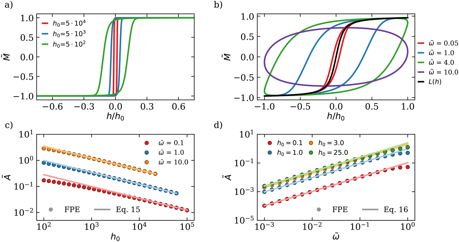
 and h0 varies with high values. In panel (b), h0 = 25 is fixed and the loops are computed for various values of
  . The static response described by the Langevin equation L(h) is shown as a black line. (c) Variation of the AC magnetic hysteresis area with h0 for large values and different values of
  . (d) AC magnetic hysteresis area as a function of
  in the low-frequency regime
  for various values of h0. In panels (c) and (d), the dots indicate the results obtained by solving the FPE and the lines indicate the predictions of eqn (15) and (16), respectively.
 because the magnetization efficiently responds to the time variation of the applied field; in the limit
  , the hysteresis vanishes and the system magnetization M follows the static behavior described by the Langevin function (Fig. 4b, black line). High intensity h0 > 1 and low frequency
  are well outside the LRT. Fig. 4d shows the scaling law for the area in this region, which follows as:
 , the external field oscillates faster than the magnetic relaxation time, τB, and the magnetic moments can no longer follow the rapidly changing field. This leads to a smaller magnetization and a reduced AC magnetic hysteresis area. At low field values h0 < 1 the maximum area takes place for
  . This result is consistent with a sort of stochastic resonance correctly captured by LRT (eqn (14)), which predicts more dissipation when the relaxation rate 1/τB coincides with ω. However, the non-linear response to high external fields alters the location of the maximum dissipation towards larger frequencies
  , as shown in Fig. 3a and d (black dashed line). The LRT also severely fails in this regime as its maximum area increases without bounds with h0, as
  . However, as previously noted (Fig. 4b and 3c), the maximum value of the non-dimensional area is capped at
  and this limit is reached for h0 → ∞ following a logarithmic trend. The agreement between
  in eqn (8) and the FPE's maximum area is perfect, as shown in Fig. 3c.
 . The collection of unknown “fundamental system's variables” is notated as
  and contains the hydrodynamic radius and magnetic moment of MNPs, the solvent viscosity, and the temperature and number of MNPs. Yet, in many practical applications, these properties,
  , are not single-valued but rather follow a distribution. We will characterize the first two moments of such distributions pi(λi): the mean 〈λi〉 and the variance σλi2. The shape of these marginal distributions pi(λi) such that p(λ) = Πipi(λi) are part of the model: typically we used a delta for single-valued variables, a Gaussian or a log–normal distribution depending on the specific variable (see the Materials and methods section). This leads to a generalization of the vector of unknown variables, which is noted as Λ = {〈λ〉, σλ}. The “theoretical” average area in dimensional units was obtained from relationship 1 weighted by p(λ; Λ) as:
 given by:
 closely match the “true” values used in the BD simulations. In all instances, the relative error remains consistently of the order of 1% or smaller for each parameter, highlighting the method's high accuracy in determining unknown system parameters.
 , and σc takes various values that are indicated in the first column


 , where the parameters with superscript ‘0’ correspond to values for p-MNPs, providing a reliable initial guess. This approach restricts the parameter search to the critical region defined by previously measured values. The hydrodynamic radius values obtained through this method are presented in Table 4 (column 1) and compared with NTA measurements.

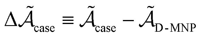 for H0 = 4 kA m−1 (e) and H0 = 24 kA m−1 (f) by comparing the cases of f-D-MNPs (stars) and f-D-MNPs + 2 μM (diamonds).
 between the dextran-coated D-MNPs and the cases with functionalized particles (f-D-MNPs) and adsorbed proteins (f-D-MNPs + 2 μM). These differences are subtle and depend on a non-trivial way with the field intensity and the frequency. For instance, the difference (and thus the resolution) is quite poor
  if one uses high frequencies and low intensities (linear regime, H0 = 4 kA m−1) or, also, when using low frequencies and high intensity (H0 = 24 kA m−1). This illustrates the importance of analyzing a broad range of frequencies and intensities to ensure consistent and accurate parameter estimations.


 .
.
 ,
,


 represents the cost function (eqn (18)). For this problem, the loss function used was the sum of relative error between the experimentally measured area (Aexp(ξ(i))) and the predicted area for a given set of parameters (A(Λ, ξ(i))) for each measured area. A detailed explanation of the fitting algorithm can be found in the ESI† and the source code used for the fitting process is available in the following repository.56


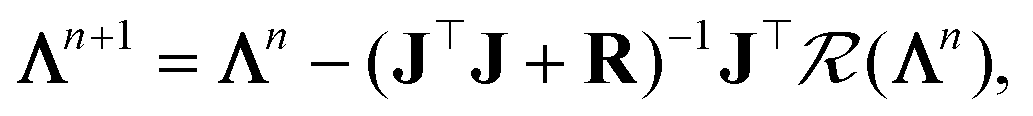
 is a regularization matrix introduced to ensure that J⊤J is invertible. The iterative algorithm continues until the norm of the residual vector is smaller than 10−5.


 and
and  are related to the mean and standard deviation of the distribution as follows:

 . When calculating the total area of a particle system using eqn (1), it is important to note that the area is normalized by m0, which depends on rc. Therefore, the total area is given by the expression:
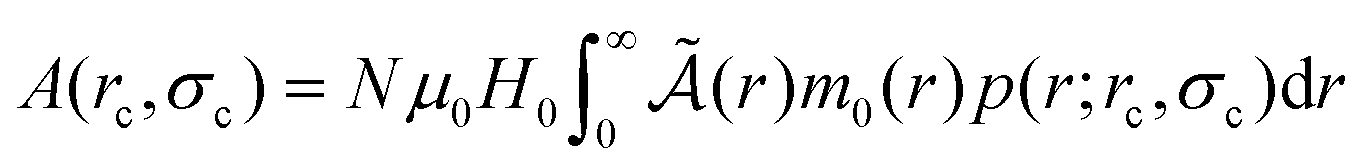
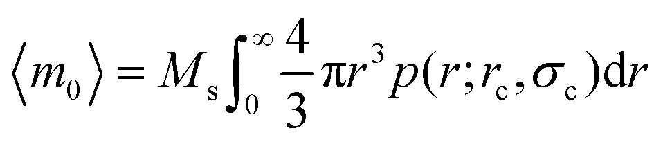

 , along with the stochastic torque arising from random collisions between the solvent molecules and the particles.

 is a vector of independent Wiener increments consisting of three random components with zero mean and unit variance. To solve this stochastic differential equation, the Euler–Maruyama algorithm was employed, as detailed in ref. 67 and further described in ref. 68.

 , eqn (41) is no longer valid, as it leads to negative probabilities. In such cases, the particles are initially aligned with the z-axis.