Expediting field-effect transistor chemical sensor design with neuromorphic spiking graph neural networks

Abstract

Improving the sensitive and selective detection of analytes in a variety of applications requires accelerating the rational design of field-effect transistor (FET) chemical sensors. Achieving high-performance detection relies on identifying optimal probe materials that can effectively interact with target analytes, a process traditionally driven by chemical intuition and time-consuming trial-and-error methods. To address the difficulties in probe screening for FET sensor development, this work presents a methodology that combines neuromorphic machine learning (ML) architectures, specifically a hybrid spiking graph neural network (SGNN), with an enriched dataset of physicochemical properties through semi-automated data extraction using large language models. Achieving a classification accuracy of 0.89 in predicting sensor sensitivity categories, the SGNN model outperformed traditional ML techniques by leveraging its ability to capture both global physicochemical properties and sparse topological features through a hybrid modeling framework. Next-generation sensor design was informed by the actionable insights into the connections between material properties and sensing performance offered by the SGNN framework. Through virtual screening for the detection of per- and polyfluoroalkyl substances (PFAS) as a use case, the effectiveness of the SGNN model was further validated. Density functional theory simulations confirmed graphene as a promising active material for PFAS detection as suggested by the SGNN framework. By bridging gaps in predictive modeling and data availability, this integrated approach provides a strong foundation for accelerating advancements in FET sensor design and innovation.

---

Design, System, Application

For sensitive and specific analyte detection in a variety of applications, such as environmental monitoring and biomedical diagnostics, field-effect transistor (FET) chemical sensors are promising technologies. However, finding the best probe materials is necessary to achieve high performance in these sensors; this process has historically been limited by trial-and-error methods and small datasets. A neuromorphic spiking graph neural network (SGNN) framework that connects material-level insights with device-level functionality is presented in this work. The framework predicts sensor sensitivity with a high accuracy and offers practical design guidelines for maximizing FET sensor performance by combining enriched datasets with hybrid machine learning models. By using virtual screening for the detection of per- and polyfluoroalkyl substances (PFAS), we validate this methodology and show that graphene is a promising option for high-sensitivity probes. This study shows how a data-driven design approach can accelerate the development of FET sensors, allowing for scalable fabrication and optimization for next-generation sensing applications in the industrial, medical, and environmental fields.

Introduction

Field-effect transistor (FET) chemical sensors have become a promising technology for the sensitive and label-free detection of biological and chemical analytes in liquid and gas phases.^1–3 They are very appealing for applications ranging from biomedical diagnostics to environmental monitoring because of their capacity to directly translate chemical/biological interactions at the sensor surface into electrical signals.^4–6 As shown in Fig. 1a, the typical structure of a chemical FET sensor consists of a channel material (e.g., graphene) connected by source and drain electrodes, where recognition probes are immobilized on the channel surface to interact with target analytes in liquid or gaseous media. These chemical interactions at the sensor interface induce carrier transport in the channel material, which can be monitored through electrical measurements (Fig. 1b). However, despite notable progress, several challenges impede the broad use and optimal performance of FET chemical sensors. Achieving high sensitivity and selectivity is one of the main obstacles.^7,8 In environments with high ionic strength, such as physiological fluids, the Debye screening effect shortens the effective sensing distance of FET sensors, which lowers their sensitivity to target analytes that are not immediately adjacent to the sensor surface.^9,10 The sensor response is further complicated by non-specific molecule binding, which results in false positives and reduced specificity.^11,12 Furthermore, reproducibility and stability continue to be major issues.¹³ Frequent calibration may be required for FET sensors due to their susceptibility to signal drift and hysteresis over time.^14,15 Environmental factors that can negatively impact sensor performance, such as variations in temperature, pH, and light exposure, can produce inconsistent and untrustworthy results.^16,17 Significant challenges are also presented by fabrication issues.¹⁸ The quality of the materials used, such as silicon nanowires or graphene, has a significant impact on the performance of FET sensors.^19,20 It is technically challenging and frequently not scalable to produce these materials with the necessary purity and structural integrity. There is still a need to develop scalable, reproducible, and affordable fabrication methods without compromising sensor performance.²¹ Furthermore, it is difficult to interpret data from FET sensors. It is challenging to separate responses based solely on the target analyte because the signals produced are impacted by several interrelated factors. This intricacy restricts the sensor's use in practical situations and calls for advanced signal processing methods.²² Fundamental material science problems at the atomic/molecular-level design are at the heart of these difficulties, as they ultimately control the overall functionality of FET chemical sensors. Chemical intuition and corresponding trial-and-error testing have historically played a significant role in the creation of new materials and sensor designs; these approaches are time-consuming and frequently ineffective.^23,24 To overcome current constraints, new approaches that can expedite the research and rational design are desperately needed.

Fig. 1 (a) Schematic illustration of a typical FET chemical sensor showing key structural components. (b) Simplified pipeline demonstrating the sensing mechanism from probe–target–medium interactions to electrical signal output.

Researchers have used modeling tools to solve these issues and offer more trustworthy advice for sensor design. Conventional computational techniques, such as molecular dynamics (MD) simulations and density functional theory (DFT) calculations, have been crucial in expanding our knowledge of material properties at the atomic and molecular levels.^25,26 However, the application of these approaches to device-level FET sensor modeling remains limited to qualitative analysis. Numerous real-world variables, including interactions with the environment, flaws caused by manufacture, and changing operating circumstances, are frequently overlooked by them. These models' predictive potential and suitability for creating sensors with the best possible performance are constrained by their qualitative nature.^27–29 Alternative approaches that can bridge these materials insights and device-level functionality are required, as evidenced by the discrepancy between theoretical predictions and real-world applications.

The absence of high-throughput experimental synthesis and evaluation techniques for FET sensors further complicates the shift from material-level insights to device-level predictions. The intricate assembly procedures of FET sensors prohibit such high-throughput methods, in contrast to other domains where automation and robotics have made it possible for quick screening and device and material optimization.^30–33 Implementing automated, large-scale experimentation is difficult due to the complex fabrication processes and the devices' susceptibility to slight production differences. The investigation of novel material combinations and device architectures is restricted by this bottleneck, which also slows down the rate of invention.³⁴ As a result, the development cycle for FET sensors continues to be drawn out, and the creation of new, high-performance sensors is severely hampered.

Currently, researchers in chemistry/materials science and engineering have gradually embraced machine learning (ML) approaches.^35,36 ML models could rapidly uncover the underlying pattern to speed up the discovery processes based on the data from, as we previously mentioned, either significant number of theoretical simulations³⁷ or experiment trials.³⁸ However, when it comes to FET sensors, ML is mostly used to analyze real-time operating data, calibrate devices, and improve performance by correcting signal drift.^39,40 Although this use of ML increases the accuracy and reliability of sensors, it ignores the urgent need to find new materials or probe–target combinations that could substantially improve sensor performance. The potential of ML to direct the rational design and development of next-generation FET chemical sensors remain undeveloped due to the current focus on operational data analysis.⁴¹ The lack of extensive, consistent datasets is the reason why researchers in the field steer clear of such investigation. The scarcity of large-scale, high-quality data hinders the development of robust data-driven ML models capable of both making accurate predictions and providing meaningful insights for bottom-up sensor design. Therefore, there is a huge opportunity to broaden the use of ML beyond its current function as a data interpretation tool to that of a catalyst for meta-level innovation.

To overcome the challenges discussed above, we have proposed a novel solution as shown in Fig. 2. It streamlines from data preparation (phase I–III) to ML modeling (phase IV) and finally application in obtaining domain insights for FET chemical sensors as well as virtual screening of probe candidates (phase V–VI). Addressing the issue of data scarcity, we employed large language models⁴² (LLMs) in a semi-automate manner by automatically parsing the vast corpus of publications into structured data with a carefully designed structure incorporating necessary information for downstream ML. In addition, manual inspection and correction were further conducted to ensure the reliability of the extracted data and mitigate potential inaccuracies from LLMs. To further enhance the quality of the dataset, we enriched the extracted data with substantial physicochemical properties from established databases and computational tools – including experimentally measured values from sources like PubChem, as well as theoretically calculated descriptors using cheminformatics tools like RDKit – grounding the information in experimentally verifiable parameters.

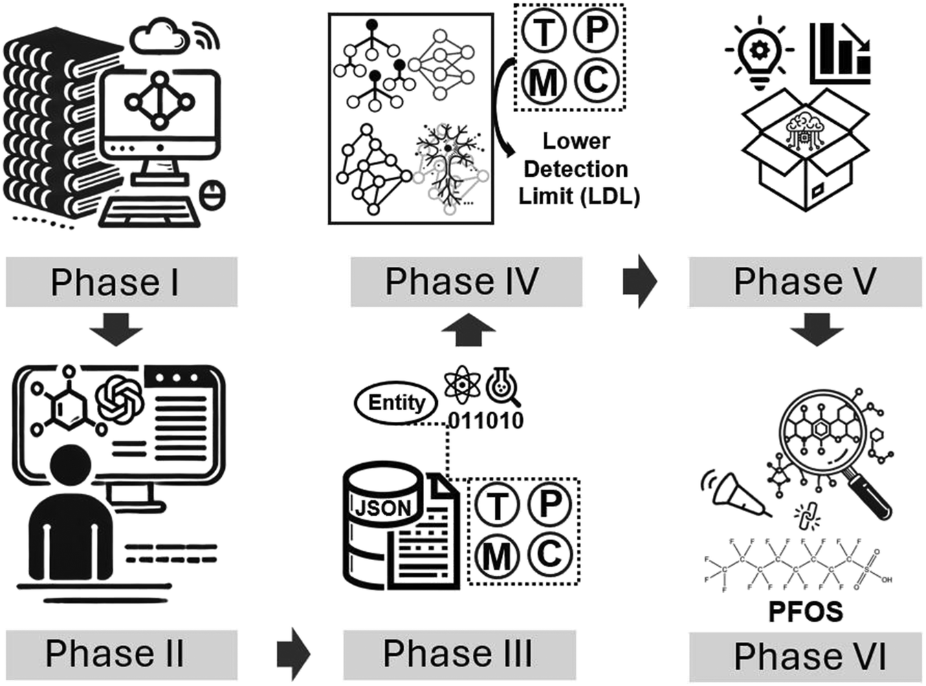Fig. 2 Overview of the different phases of this work. Phase I: literature mining and DOI compilation from scientific databases using query strings and cloud-based data extraction. Phase II: semi-automated data extraction with LLM assistance and manual validation to compile experimental parameters. Phase III: data transformation and enrichment by converting experimental records into JSON format and integrating physicochemical properties. Phase IV: development and implementation of machine learning models including SGNN to predict lower detection limit (LDL) categories based on target (T), probe (P), medium (M), and conditions (C) parameters. Phase V: analysis and interpretation of the best-performing model to derive physicochemical insights and design rules. Phase VI: validation through virtual screening and DFT simulations for PFOS detection, demonstrating a practical application of the framework.

For predictive modeling, we used several ML algorithms. In particular, we developed a novel hybrid model combining a graph neural network⁴³ (GNN) and a neuromorphic spiking neural network^44–46 (SNN) for learning physicochemical properties and structural characteristics of the substances,⁴⁷ respectively. The spiking graph neural network (SGNN) model, as a combination of both SNN and GNN, has shown a promising performance for classifying FET chemical sensors into categories ranging from very high to very low sensitivity. When testing the model's ability to correctly predict sensor sensitivity categories, it successfully identified the correct category in 89% of the cases, substantially outperforming other ML architectures in comparison (a random guess baseline would only achieve 22% accuracy). From the as-trained best-performing SGNN model, we could derive further physicochemical insights – e.g., most impactful features for determining sensing performance – that can be used for guiding FET sensor design. Finally, we were able to broaden its impact by using the domain knowledge-informed SGNN model to find promising probe candidates toward certain challenging contaminants that have not been fully studied in the field. Perfluorooctane sulfonic acid (PFOS)⁴⁸ is a typical per- and polyfluoroalkyl substance (PFAS), also known as “forever chemicals”,^49,50 that widely exists in many bodies of water. Through comprehensive dry lab DFT simulations, we successfully validated new candidate that might offer high sensitivity and selectivity toward PFOS based on the SGNN prediction.

Results and discussion

Data preparation and knowledge integration

To effectively address the data scarcity that impedes ML applications in FET sensor design, we leveraged LLM to semi-automate the extraction of experimental data from a vast corpus of publications through prompt engineering. While LLMs significantly accelerate data collection, they can introduce inaccuracies due to their limitations in understanding physical and chemical principles. To mitigate this, we enriched the extracted data with substantial physicochemical descriptors retrieved from established databases, grounding the dataset in experimentally verifiable parameters. This comprehensive dataset not only expedited the data preparation process but also enhanced the quality and reliability necessary for robust ML modeling.

Building upon the initial data extraction, we systematically transformed and enriched the dataset to prepare it for ML analysis. We began by compiling a comprehensive list of publications related to FET sensors from scientific databases using customized query strings. Utilizing LLMs, we semi-automated the extraction of key experimental parameters from these publications, including sensor types, detection targets, detection limits, probe materials (the functional materials that directly interact with and recognize target analytes), operational conditions, and mediums. To ensure data quality and consistency, we performed manual validation to correct inaccuracies, standardize units, and unify terminologies. This included converting detection limits reported in various units to a common scale (e.g., parts per million) and resolving ambiguities in chemical nomenclature. We also excluded entries with complex substances that lacked retrievable properties or those that did not align with our focus. This rigorous process resulted in a curated dataset of 1433 data entries extracted from 1192 publications, providing a solid foundation for subsequent modeling efforts.

ML modeling

To predict the sensing performance of FET chemical sensors, we developed ML models that map the physicochemical descriptors of probe materials, detection targets, and operational mediums to the sensors' lower detection limits (LDLs). Recognizing the limited size of the initial dataset, we applied data augmentation techniques to enhance its diversity and robustness. We assumed that small perturbations in experimental conditions—such as minor variations in temperature (±10%) for gas-phase sensors or slight pH adjustments (±0.5 units) for liquid-phase sensors—would not significantly diverge the classification of detection limits. By introducing these controlled variations, we generated additional data points without altering the underlying detection limit categories, effectively expanding the dataset to over 10 000 unique entries. To ensure rigorous evaluation, we performed train-test splitting before augmentation and assessed the model using both the augmented test set and the original, non-augmented data. This methodology ensures a more rigorous assessment of the model's performance under real experimental conditions rather than artificially perturbed data. Furthermore, we transformed continuous detection limit values into discrete categories based on logarithmic scales, framing the problem as a classification task rather than a regression one. Specifically, the continuous LDL values were discretized into five discrete ranges: category 5 for values ≥1 ppm, category 4 for 0.1–1 ppm, category 3 for 0.001–0.1 ppm, category 2 for 0.00001–0.001 ppm, and category 1 for values <0.00001 ppm, where lower category numbers correspond to higher sensitivity (i.e., category 1 represents the highest sensitivity and category 5 the lowest). This transformation facilitated the use of classification algorithms, and improved the models' ability to generalize across different sensor configurations. The distribution in Fig. S1 and Table S1† shows a baseline accuracy of 21.99% for random guesses.

Each data sample (experimental trial) was encoded as a JavaScript Object Notation (JSON) object, with blocks for target (T), probe (P), medium (M), and conditions (C)—as we can see in Fig. 3a. Additionally, as illustrated in Fig. 3b, the blocks target, probe, and medium are each composed of a set of one or more substances, described by their names, substance types (e.g., small molecule, inorganic solid, polymer), and other relevant corresponding descriptors (e.g., molecular mass, volume, topological polar surface area namely TPSA, and also sparse fingerprints like Morgan binary fingerprint which is typically used for molecule virtual screening⁵¹). The conditions block, on the other hand, is made of key values describing how the experimental measurement environment: operating temperature, maximum and minimum pH—all of them referring to the electrolyte medium.

Fig. 3 Data encoding description. (a) Overview of the JSON object (representing a sensing experimental trial) composed of T, P, C, and M blocks and LDL values. (b) Breakdown of the data structure of substances composing T, P, and M blocks and discretized LDL category values. (c) Naïve sequential encoding (JSON object turned into a vector) used in gradient boosting, CatBoost, XGBoost, and MLP through sequential concatenation. (d) Graph encoding (JSON object turned into a graph) used in the vanilla GNN and in part of the SGNN.

Given this data structure, we then proceeded to encode the data samples in a specific way that best fits each state-of-the-art baseline classification algorithm: (vanilla) gradient boosting, CatBoost, XGBoost, multi-layer perceptron (MLP), GNN, SNN, and SGNN. In all cases, the output is always an integer 1–5 that corresponds to the LDL category as defined. For traditional ML algorithms (gradient boosting, CatBoost, XGBoost, and MLP) which require vectorized input, numerical features from each JSON object were concatenated into fixed-length input vectors. As shown in Fig. 3c, this straightforward encoding approach included padding to ensure uniform vector dimensions across all inputs. The graph encoding scheme for the vanilla GNN (and part of the SGNN) is represented by Fig. 3d. Each node (T, P, M, C) is made of their respective features and—analogously to the sequential encoding—we performed data padding to make sure all nodes had the same dimension. The proposed architecture—T, P, M fully connected, and C connected only to M—was derived from the observation that target, probe, and medium greatly interact with each other for determining the LDL value, while the conditions node (pH, temperature) mainly influences the sensing performance through its direct effects on the medium's properties. While minor thermodynamics effect may exist directly on target and probe, the testing conditions would majorly determine the aqueous/gaseous sensing environment by ionic strength, charge distribution, and molecular diffusion.

Given their proficiency with complex, graph-structured data, GNNs effectively modeled the interconnected chemical and material properties of FET sensors. Compared with the sequential encoding method (Fig. 4a), the graph-based encoding for GNN (Fig. 4b) better captured interactions between T, P, and M descriptors, aligning with the physicochemical process of sensor probe detecting target in the medium.

Fig. 4 Comparison of ML modeling strategies. (a) Sequential encoding and architecture. (b) Vanilla GNN encoding and architecture. (c) SGNN architecture: each JSON object was split into graph representation with only global physicochemical properties descriptors, plus spike-like data corresponding to the sparse fingerprint for the topology and geometric description. Both GNN and SNN outputs are then combined via a fusion layer, which results in a 5-dimensional output corresponding to the discrete LDL categories.

To further enhance the model, we integrated an SNN (based on standard “leaky-integrate-and-fire” mechanism as shown in Fig. S2†) with the GNN model, resulting in the SGNN model. As illustrated in Fig. 4c, our proposed SGNN further naturally handles sparse node features such as the Morgan fingerprint, a molecular descriptor representing the structure and connectivity of a molecule by encoding information about atomic neighborhoods. Specifically, the Morgan fingerprints use a binary string based on the presence or absence of different substructures and atomic environments at various topological distances from each atom in the molecule. Hence, these binary fingerprints in the T, P, and M nodes are treated as spike trains, as we show in the bottom pipeline of Fig. 4c. In the meantime, the upper pipeline maintains the graph representation of global physicochemical properties (e.g., TPSA, volume, mass), similar to the vanilla GNN encoding method (Fig. 4b). The key difference is that the vanilla GNN encodes all descriptors together, while the SGNN separates global descriptors and sparse fingerprints to leverage the strengths of both GNN and SNN.

LDL classification

After defining the data encoding for each algorithm, we split the dataset into an 80 : 20 ratio (training-test) and proceeded to run all the discussed methods. We set the number of iterations to 200 and the learning rate to 0.001, and measured classification metrics such as accuracy (portion of accurately classified cases), F1 score (harmonic mean of precision and recall), precision (the proportion of correctly predicted positive labels among all labels that the model predicted as positive), and recall (measures the model's ability to identify all instances of a particular class). Given the goal of accurately identifying the LDL category of each sensor belongs to, we focused primarily on accuracy to compare the performance of different algorithms. Additionally, it is worth noting that all models have specific hyperparameters that can be tuned in order to maximize the classification accuracy. We used the state-of-the-art Bayesian optimization framework BALLET⁵² to obtain the optimum set of hyperparameters more effectively for each model.

As shown in Fig. 5, SGNN (Fig. 4c) significantly outperformed the vanilla GNN (Fig. 4b) and other algorithms relying on sequential encoding, including (vanilla) gradient boosting, XGBoost,⁵³ CatBoost,⁵⁴ and MLP. Even when using only the bottom pipeline of the SNN (i.e., the vanilla SNN with sparse, geometric fingerprints as spike train input), the classification performance exceeded that of the vanilla GNN, which utilized both data components. This result confirms our expectation that using GNNs for dense physicochemical features and SNNs for sparse geometric descriptors is superior to employing a single encoding method for all features. Given the baseline accuracy of 0.22 for random guessing, SGNN's 0.899 accuracy demonstrates its reliability and suitability for this classification task. On top of that, the combination of GNNs and SNNs offers additional advantages such as enhanced temporal information processing⁵⁵ and energy-efficient models for learning large-graph data.⁵⁶ For those reasons, the proposed SGNN, along with potential future variations, represents a powerful tool for capturing the complex interactions within FET sensors and offering predictive insights for the rational design of novel materials and device architectures.

Fig. 5 Average LDL category classification metrics for SGNN, SNN, GNN, XGBoost, CatBoost, gradient boosting, and MLP considering both the augmented and original test sets. The error bars represent the standard deviation obtained after 10 trials.

Feature importance ranking

After establishing SGNN as the best performing model optimized via the BALLET framework, we aimed to identify the most impactful features contributing to LDL classification. Each data entry includes hundreds of descriptors spanning physicochemical properties, and topological, structural, and geometric fingerprints. Analysis in identifying the most impactful features would greatly help us to obtain additional insights into the designing rules for FET sensors.

There are multiple ways to perform feature selection. In our case, we used integrated gradients⁵⁷ and Shapley values⁵⁸ for determining each feature's contribution to the prediction for each sample. For both approaches, we obtained the relative frequency (a number between 0 and 1) of each feature to be in the top 10 most relevant features. As described in the Methods section in ESI,† we also employed random matrix theory (RMT) techniques—such as the Marchenko–Pastur law and sparse principal component analysis (PCA)—to further verify the feature selection results obtained via integrated gradients and SHAP values.

Fig. 6 contains the breakdown of the final results—both globally and within each block (for target, probe, medium, conditions). As suggested by these results, the target block contains the most important features overall: mass being the most important, followed by volume, TPSA and complexity. Probe is also an important block, contributing to the LDL prediction via its space group number (SGN), bulk modulus, shear modulus, and mass. Temperature and pH value in the condition block are highly significant, consistent with the chemical intuition. Temperature influences thermodynamics, particularly in gas sensing, where it affects sensor response.⁵⁹ In liquid environments, pH is crucial as it impacts the charges of probe molecules, influencing their isoelectric points.⁶⁰ Finally, medium properties (XLogP namely octanol–water partition coefficient with atom-additive approach, TPSA, mass) are far less impactful in the LDL category prediction. Such results are also consistent with the chemical intuition and domain consensus of those sensing phenomena.

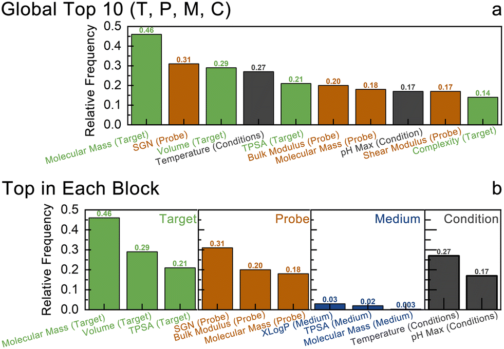Fig. 6 Feature importance analysis results: (a) global and (b) by specific node blocks based on SHAP values and integrated gradients analysis.

In FET chemical sensors, the detection limit is influenced by various factors related to the target analyte, the probe material, and the surrounding medium. The mass, volume, and TPSA of the target analyte are critical, as they affect how the analyte interacts with the sensor's probe, thereby impacting sensitivity. Larger mass and volume can enhance van der Waals interactions, while a higher TPSA may increase hydrogen bonding potential, both of which can strengthen binding affinity.^61,62 The probe's properties, such as its bulk modulus and space group number, determine its mechanical stability and crystalline structure, influencing its ability to transduce chemical interactions into electrical signals.^63,64 The medium's characteristics, including pH and temperature, can alter the analyte's ionization state and the probe's surface chemistry, affecting the overall sensor response.⁶⁵ However, the medium often serves as a passive environment, making its features less impactful compared to those of the target and probe. Understanding these relationships aligns with established principles in sensor design, where the interplay between analyte properties and probe characteristics is pivotal for achieving optimal performance. Moreover, by such black-box interpretation analysis, we validated that the SGNN effectively captures domain knowledge, making it a reliable predictor for designing novel materials.

PFOS screening

Finally, for the exploration of the realistic application impact of our model, we applied the previously highlighted SGNN model with the optimal hyperparameters choice for screening the potentially promising probe material for the detection of PFAS chemicals in water through the FET sensor device. After fixing a given conditions block (25 °C, pH = 7), we scanned through all the possible probe substances that have been recorded in our dataset and computed the corresponding LDL category. As shown in Table S2,† 7 different typical PFAS chemicals are selected as target, then the probe substances predicted by the SGNN model which has learnt domain knowledge to possess very low LDL (high sensitivity) category would be treated as promising candidates for detection. It is worth mentioning that the similarities between those molecules stem from their common perfluorinated carbon chains and functional groups (e.g., carboxylic acid, sulfonic acid).^66,67 For these reasons—and their high environmental and health relevance—such molecules are representatives of the PFAS family, with varying degrees of bioaccumulation and toxicity.^66–68

As a result, we could find highly consistent predictions. The top 4 most recurrent probe materials associated with this behavior were: graphene, zinc oxide, aluminum oxide, and carbon nanotube. This result can also be analyzed from the recall perspective, since it measures how well the SGNN has identified all correct instances by computing the fraction of true positives relative to the total of true positives and false negatives. In this case, a true positive corresponded to a category 1 probe material that was classified as such, while a false negative represented a category 1 (high sensitivity) probe missed by our model. Since recall values oscillated between 0.877 and 0.899 through our modeling results (Fig. 5), we concluded that, with high probability, we identified most of the best category 1 probe materials. Had we used algorithms with a smaller recall, it would be more significantly likely to miss a promising potential candidate.

In order to validate the practical values of these predictions which originate from our advanced ML modeling on domain knowledge, dry lab simulations of theoretical sensing performances are conducted. We choose PFOS as the prototypical PFAS analyte and sodium dodecyl sulfate (SDS) as the interferent, respectively, based on previous work.⁶⁹ While binding energies with PFOS (ΔE_PFOS) and SDS (ΔE_SDS) are considered qualitative representations of sensitivity, their difference (ΔΔE_PFOS–SDS = ΔE_PFOS − ΔE_SDS) is used for selectivity evaluation. First for initial screening, we conducted ab initio simulations in the standard vacuum condition with periodic boundary conditions considering that zinc oxide (ZnO) and aluminum oxide (Al₂O₃) are inorganic materials. Beyond the above mentioned 4 SGNN-predicted substances, 6 more substances that have been reported as probe for PFOS sensing are also included for comparison:⁷⁰ β-cyclodextrin (β-CD),⁷¹ ferrocenecarboxylic acid (FcCOOH),^72,73 1H,1H,2H,2H-perfluorodecanethiol (FDT-SAM),⁷⁴o-phenylenediamine (o-PD),⁷³ polyaniline⁷⁵ (represented by aniline), and polypyrrole⁷⁶ (represented by pyrrole). As shown in Fig. 7, in this simulation environment, most substances would show higher propensity to combine with SDS rather than PFOS, except for FcCOOH showing an exceptional 0.58 eV advantage of PFOS over SDS. Among the rest, though two inorganic substances predicted by SGNN: Al₂O₃ and ZnO, have shown exceptional binding energies (between 2.42–3.79 eV) toward the two analytes, their preference is on SDS over PFOS. In comparison, the other two: graphene and single-walled carbon nanotube (SWNT) possess the lowest degree of such disadvantage. To further comprehensively examine the binding behavior, quantum chemistry DFT simulation with a higher precision is initially conducted in two different simulation environments: default vacuum and implicit water solvent field. As summarized in Fig. S3a and b,† the results in different scenarios are generally consistent. Although FcCOOH's selectivity advantage is again confirmed, we could observe that graphene predicted by our SGNN model, followed right behind in terms of ΔΔE_PFOS–SDS. To further explore higher fidelity, explicit solvent cluster: water molecules are added into the system. As shown in Fig. S3c,† though FcCOOH is still promising, graphene now shows a higher ΔΔE_PFOS–SDS of 7.94 eV overtaking that of FcCOOH's. To obtain deeper insights into the difference in binding mechanism, we discussed the highest occupied molecular orbital (HOMO) and lowest unoccupied molecular orbital (LUMO) in Fig. S4.† It was concluded that FcCOOH likely has stronger electronic coupling and orbital interactions with PFOS, indicated by drastically changed gap values—mostly due to its ability to engage in hydrogen bonding and electrostatic interactions with PFOS's sulfonic acid headgroup. In contrast, graphene's mechanism might be through weaker interactions like π–π stacking, hydrophobic interactions, and physisorption.^77,78 This results in minimal HOMO–LUMO gap changes despite favorable binding energies. By combining these two probes—e.g., grafting FcCOOH onto a graphene channel—we can leverage FcCOOH's molecular specificity as well as graphene's high surface area, conductivity, and broad adsorption capacity. This integration increases sensitivity and selectivity, yielding a more stable and reliable sensing platform for PFOS detection in real-world scenarios.

Fig. 7 (a) ΔE_PFOS and ΔE_SDS, (b) ΔΔE_PFOS–SDS of different probe substances in ab initio simulation with periodic boundary condition.

To further validate our hypothesis, we investigated PFOS binding to our probe systems under explicit solvent AIMD conditions. The results—illustrated in Fig. S5†—clearly show that while FcCOOH alone exhibits a significant binding advantage, the graphene–FcCOOH hybrid displays an even stronger relative binding affinity for PFOS. These findings support our prediction of a synergistic effect between graphene and FcCOOH for enhanced PFOS sensing.

In general, our dry lab simulation results qualitatively support graphene as a promising candidate for PFOS sensing against SDS, showcasing potentially comparable selectivity and sensitivity to FcCOOH by previous reports^72,73 validated in this study. The robustness, scalability, and environmental compatibility of graphene further highlight their practical advantages, aligning with the overarching goal of real-world sensor development.⁷⁹ Moreover, due to its superior electrical properties, graphene itself is already frequently used as the two-dimensional material as the channel of FET sensors. Our study suggests that with potentially straightforward modifications of currently well-established graphene-based FET sensors, it may be possible to develop effective PFOS sensors-though here we have only demonstrated using SDS as one representative interferent.

Conclusion, outlook, and future work

This work shows how to use an integrated ML framework to advance the rational and data-driven design and optimization of FET chemical sensors in a revolutionary way. By utilizing a neuromorphic SGNN architecture and enriched datasets, we achieved notable advancements in sensor sensitivity classification, attaining an accuracy of 0.89 and outperforming traditional ML techniques. In addition to predictive modeling, the SGNN framework uncovered physicochemical insights that bridge fundamental material properties to sensor performance, thereby informing both sensitivity and selectivity optimization strategies. As a result of these developments, graphene was identified as a promising probe material for PFOS detection, which was confirmed by dry lab simulations. This study provides a robust foundation for accelerating FET sensor innovation by filling important gaps in data scarcity and predictive capabilities. Our future work would include validating the two theoretical probes in devices and their combination, e.g., grafting and modification of FcCOOH on graphene-based FET channels to make full use of their binding mechanism for maximum sensing performances.

Our integrated approach advances FET sensor development through two key contributions: addressing the data scarcity challenge and providing a predictive framework for screening novel materials and architectures. In summary, we present a comprehensive methodology that bridges the gap between the need for comprehensive, high-quality data and the development of advanced ML models for FET chemical sensors' design and optimization. By integrating neuromorphic SGNNs with enriched datasets, we offer a powerful tool for researchers to navigate the complexities of FET sensor development and to unlock new possibilities in sensor technology.

Despite these advancements, there is still room for improvement. The current SGNN architecture and dataset oversimplify the graph representation of sensing systems, potentially overlooking complex interactions between targets, probes, and media. For instance, under varying pH, ionic strength, and temperature—will be essential for refining model predictions and ensuring real-world relevance. Enhanced graph architectures that capture multi-level relationships and complex interactions may provide more comprehensive understanding of the underlying mechanisms.

Furthermore, the dataset's lack of temporal dynamics restricts the SNN's ability to fully utilize its event-driven capabilities. In addition to this aspect, while the SNN we implemented relies on intrinsic spiking features, there weren't any explicit time-dependent or event-driven features in our dataset, which also limits the SNN impacts. More thorough modeling of dynamic sensor behaviors would be possible with the inclusion of time-series data, such as response kinetics and recovery times or signal drift patterns over operational lifetimes. The combination of more flexible, hierarchical graph representations and timeseries data—accounting for dynamic behaviors—is a research direction that we will pursue in future work, allowing us to generalize the SGNN framework across different types of sensing design.

Additionally, real-world experiments—as planned for future work—will enhance the robustness and generalizability of our proposed SGNN framework. While our current simulation results (under realistic solvation conditions) successfully validate our model's predictions, wet lab experiments will serve as the ultimate benchmark, being the final step to close the loop and confirm the SGNN results.

Regarding alternative applications, one promising direction is biosensing.^80,81 The proposed SGNN framework could indeed be adapted to optimize the sensing design to detect biomarkers—e.g., proteins, nucleic acids, metabolites—or even pathogens (via viral or bacterial genetic material).^80,81 This application would require biological datasets with interaction patterns between proteins, DNA/RNA sequences, and sensor surfaces. In this context, we could encode, for instance, enzymatic activity features as a graph representation, while using the SNN to represent the biomolecular temporal dynamics. On top of that, bio-sensing applications can also include wearable devices⁸²—especially if we use 2D materials due to their flexibility^82,83—for real-time monitoring of glucose, lactate, and cortisol levels.

In the biosensing context, it is worth understanding the relationship between our SGNN framework and some state-of-the-art models, such as AlphaFold 3.^84,85 Even though it is quite challenging to perform a fair comparison due to their substantial differences in data encoding and main objectives—classifying sensor performance based on material properties versus protein structure prediction from amino-acid sequences—we can still use our model for combining different data formats. For example, the GNN would be the “global encoder” with nodes containing global descriptors (e.g., molecular weight, polarity, charge) and edges with chemical bonding features (e.g., hydrogen bonding potentials, electrostatic interactions). The SNN, on the other hand, would serve as the “local and temporal encoder”, capturing stepwise folding kinetics and transient structural states.

Expanding the dataset to include real-world metrics, such as stability, interference effects, and automated synthesis with high-throughput validation, could transform this framework into a closed-loop system for rapid sensor development. These advancements would further enhance the design and optimization of sensors for diverse applications, extending the methodology to tackle pressing challenges in environmental monitoring and healthcare diagnostics.

Data availability

Dataset and scripts are publicly available from Github repository: https://github.com/ruiding-uchicago/Chem_FET_Sensor_ML. Methods details, supporting figures and tables (Fig. S1–S5, Tables S1–S3) are available in the ESI.†

Conflicts of interest

There is no conflict of interest for this work.

Acknowledgements

This research was supported by multiple institutional and federal grants. This project is supported by the Eric and Wendy Schmidt AI in Science Postdoctoral Fellowship, a Schmidt Sciences, LLC program. Additional support came from the University of Chicago Data Science Institute through the 2024 AI+Science Research Initiative. This work was also supported in part by the National Science Foundation Future Manufacturing project #2037026, and Robust Intelligence project #2313131. The computational work was boosted by the support from several high-performance computing resources. We acknowledge the Carbon High-Performance Computing Cluster at the Center for Nanoscale Materials, Argonne National Laboratory, supported by the U.S. Department of Energy Office of Science User Facility under Contract No. DE-AC02-06CH11357. Additional computational resources were provided by the University of Chicago's Research Computing Center through proposal #68909. We also utilized the Delta computing cluster through allocation MAT240097 from the Advanced Cyberinfrastructure Coordination Ecosystem: Services & Support (ACCESS) program, which is supported by U.S. National Science Foundation grants #2138259, #2138286, #2138307, #2137603, and #2138296.

References

1. S. Mao, J. Chang, H. Pu, G. Lu, Q. He, H. Zhang and J. Chen, Chem. Soc. Rev., 2017, 46, 6872–6904.
2. W. Fu, L. Jiang, E. P. van Geest, L. M. C. Lima and G. F. Schneider, Adv. Mater., 2017, 29, 1603610.
3. C. Dai, Y. Liu and D. Wei, Chem. Rev., 2022, 122, 10319–10392.
4. A. Panahi and E. Ghafar-Zadeh, Bioengineering, 2023, 10, 793.
5. X. Chen, C. Liu and S. Mao, Nano-Micro Lett., 2020, 12, 1–24.
6. D. Sung and J. Koo, Biomed. Eng. Lett., 2021, 11, 85–96.
7. P. Barik and M. Pradhan, Analyst, 2022, 147, 1024–1054.
8. R. F. de Oliveira, V. Montes-García, A. Ciesielski and P. Samorì, Mater. Horiz., 2021, 8, 2685–2708.
9. G. S. Kulkarni and Z. Zhong, Nano Lett., 2012, 12, 719–723.
10. N. Gao, W. Zhou, X. Jiang, G. Hong, T.-M. Fu and C. M. Lieber, Nano Lett., 2015, 15, 2143–2148.
11. C. Fenzl, C. Genslein, C. Domonkos, K. A. Edwards, T. Hirsch and A. J. Baeumner, Analyst, 2016, 141, 5265–5273.
12. J. E. Contreras-Naranjo and O. Aguilar, Biosensors, 2019, 9, 15.
13. P. Zang, Y. Liang and W. W. Hu, IEEE Nanotechnol. Mag., 2015, 9, 19–28.
14. J. M. Margarit-Taulé, M. Martín-Ezquerra, R. Escudé-Pujol, C. Jiménez-Jorquera and S.-C. Liu, Sens. Actuators, B, 2022, 353, 131123.
15. S. Jamasb, IEEE Sens. J., 2020, 21, 4705–4712.
16. B. M. Lowe, K. Sun, I. Zeimpekis, C.-K. Skylaris and N. G. Green, Analyst, 2017, 142, 4173–4200.
17. F. Vivaldi, P. Salvo, N. Poma, A. Bonini, D. Biagini, L. Del Noce, B. Melai, F. Lisi and F. D. Francesco, Chemosensors, 2021, 9, 33.
18. G. Thriveni and K. Ghosh, Biosensors, 2022, 12, 647.
19. M. Sun, S. Wang, Y. Liang, C. Wang, Y. Zhang, H. Liu, Y. Zhang and L. Han, Nano-Micro Lett., 2025, 17, 34.
20. S. Sreejith, J. Ajayan, N. V. Uma Reddy and M. Manikandan, Silicon, 2024, 16, 485–511.
21. S. E. Lowe and Y. L. Zhong, Graphene oxide: fundamentals and applications, 2016, pp. 410–431.
22. M. Kaisti, Biosens. Bioelectron., 2017, 98, 437–448.
23. S. Szunerits, T. Rodrigues, R. Bagale, H. Happy, R. Boukherroub and W. Knoll, Anal. Bioanal. Chem., 2024, 416, 2137–2150.
24. H. Shin, J. Ahn, D.-H. Kim, J. Ko, S.-J. Choi, R. M. Penner and I.-D. Kim, MRS Bull., 2021, 46, 1080–1094.
25. P. Fathi-Hafshejani, N. Azam, L. Wang, M. A. Kuroda, M. C. Hamilton, S. Hasim and M. Mahjouri-Samani, ACS Nano, 2021, 15, 11461–11469.
26. Z. Kuang, S. N. Kim, W. J. Crookes-Goodson, B. L. Farmer and R. R. Naik, ACS Nano, 2010, 4, 452–458.
27. V. Singh, S. Patra, N. A. Murugan, D.-C. Toncu and A. Tiwari, Mater. Adv., 2022, 3, 4069–4087.
28. W. Dawson, A. Degomme, M. Stella, T. Nakajima, L. E. Ratcliff and L. Genovese, Wiley Interdiscip. Rev.: Comput. Mol. Sci., 2022, 12, e1574.
29. H. J. C. Berendsen, Molecular dynamics simulations: The limits and beyond, in Computational Molecular Dynamics: Challenges, Methods, Ideas: Proceedings of the 2nd International Symposium on Algorithms for Macromolecular Modelling, Berlin, May 21–24, 1997, Springer Berlin Heidelberg, Berlin, Heidelberg, 1999, pp. 3–36.
30. A. Dave, J. Mitchell, S. Burke, H. Lin, J. Whitacre and V. Viswanathan, Nat. Commun., 2022, 13, 5454.
31. J. S. Manzano, W. D. Hou, S. S. Zalesskiy, P. Frei, H. Wang, P. J. Kitson and L. Cronin, Nat. Chem., 2022, 14, 1311–1318.
32. N. J. Szymanski, B. Rendy, Y. Fei, R. E. Kumar, T. He, D. Milsted, M. J. McDermott, M. Gallant, E. D. Cubuk, A. Merchant, H. Kim, A. Jain, C. J. Bartel, K. Persson, Y. Zeng and G. Ceder, Nature, 2023, 624, 86–91.
33. B. Burger, P. M. Maffettone, V. V. Gusev, C. M. Aitchison, Y. Bai, X. Wang, X. Li, B. M. Alston, B. Li, R. Clowes, N. Rankin, B. Harris, R. S. Sprick and A. I. Cooper, Nature, 2020, 583, 237–241.
34. M. Sedki, Y. Chen and A. Mulchandani, Sensors, 2020, 20, 4811.
35. R. Ding, J. Chen, Y. Chen, J. Liu, Y. Bando and X. Wang, Chem. Soc. Rev., 2024, 53, 11390–11461.
36. D. Morgan and R. Jacobs, Annu. Rev. Mater. Res., 2020, 50, 71–103.
37. S. P. Ong, Comput. Mater. Sci., 2019, 161, 143–150.
38. E. O. Pyzer-Knapp, J. W. Pitera, P. W. J. Staar, S. Takeda, T. Laino, D. P. Sanders, J. Sexton, J. R. Smith and A. Curioni, npj Comput. Mater., 2022, 8, 84.
39. R. Bhardwaj, S. Sinha, N. Sahu, S. Majumder, P. Narang and R. Mukhiya, Int. J. Circuit Theory Appl., 2019, 47, 954–970.
40. S. Sinha, R. Bhardwaj, N. Sahu, H. Ahuja, R. Sharma and R. Mukhiya, Microelectron. J., 2020, 97, 104710.
41. U. Yaqoob and M. I. Younis, Sensors, 2021, 21, 2877.
42. J.-J. Zhu, J. Jiang, M. Yang and Z. J. Ren, Environ. Sci. Technol., 2023, 57, 17667–17670.
43. Z. Wu, S. Pan, F. Chen, G. Long, C. Zhang and S. Y. Philip, IEEE Trans. Neural Netw. Learn. Syst., 2020, 32, 4–24.
44. J. B. Aimone, Y. Ho, O. Parekh, C. A. Phillips, A. Pinar, W. Severa and Y. Wang, Proceedings of the 33rd ACM Symposium on Parallelism in Algorithms and Architectures, 2021, pp. 35–47.
45. C. D. Schuman, S. R. Kulkarni, M. Parsa, J. P. Mitchell, P. Date and B. Kay, Nat. Comput. Sci., 2022, 2, 10–19.
46. S. R. Kulkarni, M. Parsa, J. P. Mitchell and C. D. Schuman, Neurocomputing, 2021, 447, 145–160.
47. H. L. Morgan, J. Chem. Doc., 1965, 5, 107–113.
48. Y. Deng, Z. Liang, X. Lu, D. Chen, Z. Li and F. Wang, Chemosphere, 2021, 283, 131168.
49. P. Zareitalabad, J. Siemens, M. Hamer and W. Amelung, Chemosphere, 2013, 91, 725–732.
50. H. Brunn, G. Arnold, W. Körner, G. Rippen, K. G. Steinhäuser and I. Valentin, Environ. Sci. Eur., 2023, 35, 1–50.
51. A. Cereto-Massagué, M. J. Ojeda, C. Valls, M. Mulero, S. Garcia-Vallvé and G. Pujadas, Methods, 2015, 71, 58–63.
52. F. Zhang, J. Song, J. C. Bowden, A. Ladd, Y. Yue, T. Desautels and Y. Chen, Proceedings of the International Conference on Machine Learning, 2023, pp. 41579–41595.
53. T. Q. Chen and C. Guestrin, Kdd'16: Proceedings of the 22nd Acm Sigkdd International Conference on Knowledge Discovery and Data Mining, 2016, pp. 785–794,  DOI:10.1145/2939672.2939785.
54. A. V. Dorogush, V. Ershov and A. Gulin, arXiv, 2018, preprint, arXiv:1810.11363.
55. N. Yin, M. Wang, Z. Chen, G. De Masi, H. Xiong and B. Gu, Proceedings of the AAAI Conference on Artificial Intelligence, 2024, vol. 38, pp. 16495–16503.
56. J. Li, Z. Yu, Z. Zhu, L. Chen, Q. Yu, Z. Zheng, S. Tian, R. Wu and C. Meng, Proceedings of the AAAI Conference on Artificial Intelligence, 2023, vol. 37, pp. 8588–8596.
57. X. Liu and T. Yu, presented in part at the 2007 IEEE 11th International Conference on Computer Vision, 2007.
58. W. E. Marcílio and D. M. Eler, presented in part at the 33rd SIBGRAPI conference on Graphics, Patterns and Images (SIBGRAPI), 2020.
59. S. Robbiani, B. J. Lotesoriere, R. L. Dellacà and L. Capelli, Chemosensors, 2023, 11, 514.
60. M. F. Cuddy, A. R. Poda and L. N. Brantley, ACS Appl. Mater. Interfaces, 2013, 5, 3514–3518.
61. R. Parthasarathi and V. Subramanian, Hydrogen bonding—new insights, 2006, pp. 1–50.
62. C. Tantardini, A. A. L. Michalchuk, A. Samtsevich, C. Rota and A. G. Kvashnin, Sci. Rep., 2020, 10, 7816.
63. P. Hess, Nanoscale Horiz., 2021, 6, 856–892.
64. E. Comini, C. Baratto, G. Faglia, M. Ferroni, A. Ponzoni, D. Zappa and G. Sberveglieri, J. Mater. Res., 2013, 28, 2911–2931.
65. H. A. Saputra, Monatsh. Chem., 2023, 154, 1083–1100.
66. S. Rayne and K. Forest, J. Environ. Sci. Health, Part A: Toxic/Hazard. Subst. Environ. Eng., 2009, 44, 1145–1199.
67. S. C. E. Leung, D. Wanninayake, D. Chen, N.-T. Nguyen and Q. Li, Sci. Total Environ., 2023, 905, 166764.
68. A. J. Lewis, X. Yun, D. E. Spooner, M. J. Kurz, E. R. McKenzie and C. M. Sales, Sci. Total Environ., 2022, 822, 153561.
69. S. Dasetty, M. Topel, Y. O. Tang, Y. Wang, E. Jonas, S. B. Darling, J. Chen and A. L. Ferguson, J. Chem. Eng. Data, 2023, 68, 3148–3161.
70. D. Thompson, N. Zolfigol, Z. Xia and Y. Lei, Sens. Actuators Rep., 2024, 7, 100189.
71. Y. Wang, H.-J. Jang, M. Topel, S. Dasetty, Y. Liu, M. Ateia, A. Tam, V. Rozyyev, E. Ouyang, W. Zhuang, H. Pu, S. S. Lee, J. Elam, A. Ferguson, S. Darling and J. Chen, ChemRxiv, 2024, preprint,  DOI:10.26434/chemrxiv-2024-6q6q5.
72. D. Lu, D. Z. Zhu, H. Gan, Z. Yao, J. Luo, S. Yu and P. Kurup, Sens. Actuators, B, 2022, 352, 131055.
73. R. Kazemi, E. I. Potts and J. E. Dick, Anal. Chem., 2020, 92, 10597–10605.
74. G. Moro, C. J. Dongmo Foumthuim, M. Spinaci, E. Martini, D. Cimino, E. Balliana, P. Lieberzeit, F. Romano, A. Giacometti, R. Campos, K. De Wael and L. M. Moretto, Anal. Chim. Acta, 2022, 1204, 339740.
75. T. Y. Chi, Z. Chen and J. Kameoka, Sensors, 2020, 20, 7301.
76. C. Fang, Z. Chen, M. Megharaj and R. Naidu, Environ. Technol. Innovation, 2016, 5, 52–59.
77. P.-P. Zhou and R.-Q. Zhang, Phys. Chem. Chem. Phys., 2015, 17, 12185–12193.
78. A. Pérez-Guardiola, A. J. Pérez-Jiménez and J.-C. Sancho-Garcia, Mol. Syst. Des. Eng., 2017, 2, 253–262.
79. Z. Zhu, Nano-Micro Lett., 2017, 9, 25.
80. F. Cui, Y. Yue, Y. Zhang, Z. Zhang and H. S. Zhou, ACS Sens., 2020, 5, 3346–3364.
81. A. Singh, A. Sharma, A. Ahmed, A. K. Sundramoorthy, H. Furukawa, S. Arya and A. Khosla, Biosensors, 2021, 11, 336.
82. F. Yi, H. Ren, J. Shan, X. Sun, D. Wei and Z. Liu, Chem. Soc. Rev., 2018, 47, 3152–3188.
83. H. Yang, T. Xue, F. Li, W. Liu and Y. Song, Adv. Mater. Technol., 2019, 4, 1800574.
84. R. Yin, B. Y. Feng, A. Varshney and B. G. Pierce, Protein Sci., 2022, 31, e4379.
85. J. Abramson, J. Adler, J. Dunger, R. Evans, T. Green, A. Pritzel and O. Ronneberger, et al. , Nature, 2024, 1, 1–3.

---

Footnotes

† Electronic supplementary information (ESI) available. See DOI: https://doi.org/10.1039/d4me00203b

‡ These authors contributed equally to this work.

---